Residual vectors for Alzheimer disease diagnosis and prognostication

Abstract

Alzheimer disease (AD) is an increasingly prevalent neurodegenerative condition and a looming socioeconomic threat. A biomarker for the disease could make the process of diagnosis easier and more accurate, and accelerate drug discovery. The current work describes a method for scoring brain images that is inspired by fundamental principles from information retrieval (IR), a branch of computer science that includes the development of Internet search engines. For this research, a dataset of 254 baseline 18-F fluorodeoxyglucose positron emission tomography (FDG-PET) scans was obtained from the Alzheimer's Disease Neuroimaging Initiative (ADNI). For a given contrast, a subset of scans (nine of every 10) was used to compute a residual vector that typified the difference, at each voxel, between the two groups being contrasted. Scans that were not used for computing the residual vector (the remaining one of 10 scans) were then compared to the residual vector using a cosine similarity metric. This process was repeated sequentially, each time generating cosine similarity scores on 10% of the FDG-PET scans for each contrast. Statistical analysis revealed that the scores were significant predictors of functional decline as measured by the Functional Activities Questionnaire (FAQ). When logistic regression models that incorporated these scores were evaluated with leave-one-out cross-validation, cognitively normal controls were discerned from AD with sensitivity and specificity of 94.4% and 84.8%, respectively. Patients who converted from mild cognitive impairment (MCI) to AD were discerned from MCI nonconverters with sensitivity and specificity of 89.7% and 62.9%, respectively, when FAQ scores were brought into the model. Residual vectors are easy to compute and provide a simple method for scoring the similarity between an FDG-PET scan and sets of examples from a given diagnostic group. The method is readily generalizable to any imaging modality. Further interdisciplinary work between IR and clinical neuroscience is warranted.

Introduction

Alzheimer disease (AD) is the most common cause of neurodegenerative dementia among elderly patients. It is now well recognized as a public health emergency for the 21st century. By an estimate based on data from the 2000 census, there will be 13.5 million cases by the year 2050 unless treatments are developed to prevent or slow progression of the disease (Hebert et al. 2003).

The absence of biomarkers for detecting AD and tracking its progression renders discovery of new treatments more difficult. At this time, the diagnosis cannot be made with confidence in the absence of detailed cognitive testing. These cognitive tests are time consuming and can be difficult to interpret if the participant is not adequately engaged. Some clinical trials in recent years have enrolled patients with mild cognitive impairment (MCI—a condition characterized by memory impairment without dementia) and evaluated rates of conversion from MCI to AD as an outcome measure (Salloway et al. 2004; Petersen et al. 2005; Thal et al. 2005; Feldman et al. 2007). While it is true that drugs for preventing conversion are highly desirable, conversion has some undesirable properties for an outcome measure. Conversion does not take place suddenly and can be difficult to identify with certainty. Rates of conversion are low and variable, with 6–15% of amnestic MCI patients converting to Alzheimer's disease each year. This means that large numbers of MCI patients must be recruited and followed for a long period of time before it is possible to discern a difference in conversion rates between two randomized groups of participants in a clinical trial. Biomarkers offer the hope of rapid and unambiguous diagnosis, precise tracking of disease severity, and improvements over existing methods for evaluating the efficacy of interventions.

Positron emission tomography (PET) scans for the current study were acquired using 18-fluorodeoxyglucose (FDG), and will be referred to hereafter as FDG-PET or PET scans. FDG is synthesized by replacing one of the hydroxyl groups in glucose with a fluorine atom. Despite this change, the molecule bears sufficient similarity to glucose to be taken up by living cells in proportion to their metabolic demands. The radiation emitted by the tracer after it has been absorbed by the cells can therefore be used to construct a map depicting the glucose demands of the different tissues. FDG-PET scans have a characteristic appearance that can facilitate the diagnosis of AD (Silverman et al. 2001; Drzezga et al. 2005). In addition, PET scans have clinical utility for discerning between AD and dementia caused by frontotemporal lobar degeneration (FTLD) (Foster et al. 2007). Several research studies have evaluated the utility of PET scans for diagnosing AD (Minoshima et al. 1995; Silverman et al. 2001) or for predicting the progression of MCI or AD (Chetelat et al. 2003; Drzezga et al. 2005; Landau et al. 2010, 2011; Walhovd et al., 2010). PET scans for studies such as these are often subjected to complex post-processing, such as segmentation into volumes of interest, or surface projection. The current work focuses on automatic detection of AD or elevated MCI conversion risk, making use of elementary information retrieval (IR) techniques.

IR is a broad field that is concerned chiefly with the rapid selection of relevant documents from vast databases. The documents in question are traditionally text, and this has shaped many IR techniques. The simplest approach is to formulate a query as a list of key words and to retrieve only documents that contain all of the key words. This approach does not perform well in practice, however. Another approach that is almost as simple is to arrange word counts from numerous documents in a matrix and then to treat the rows and columns of the matrix as vectors. This permits comparison of documents and queries using simple mathematical measurements on vectors, such as Euclidean distance (a generalization of the Pythagorean theorem) and cosine similarity (a measure of the angle between two vectors that is maximal when the vectors are parallel). More typically, the term-document matrix is subjected to further mathematical processing for extracting the most salient features of the data, such as singular value decomposition or latent semantic analysis (Widdows 2004). This vector-space model of information has proven to be very useful, and the possibility of extending it to retrieval of images and music is an area of active research (Casey et al. 2008; Datta et al. 2008).

The diagnosis of AD (or identification of patients who meet other clinical criteria) may be approached from an IR perspective. In this case, we wish to search a database of brain images and retrieve those images that belong to patients with AD or elderly controls. Somewhat more compelling (and more difficult) is the retrieval of scans from patients with memory impairment who are destined to develop AD. The immediate problem that arises is the formulation of the query. In text-based IR, the query is simply a list of words (such as a document) that can be converted to a vector and compared to documents in the database. The current research focuses on a relatively simple method for formulating “query” vectors from groups of PET scans and then evaluating the utility of these vectors for retrieving relevant scans (i.e., for making diagnoses or predictions on the subjects who contributed the scans).

Fig. 1 summarizes the residual vector analysis method, the first step of which is mathematically identical to computing the ordinary least squares approximation of the solution to a system of linear equations. Geometrically, the ordinary least squares approximation is the projection of one vector (composed of the values of the dependent variable) onto a space defined by other vectors (the matrix of independent variables). This projection is the linear combination of vectors from the matrix column space that is closest to the original vector. Subtraction of this projection vector from the original vector yields a residual vector that is orthogonal to all of the vectors in the matrix column space. Thus, when similarity is quantified in terms of the cosine of the angle between two vectors (i.e., zero for perpendicular vectors, one for parallel vectors), the residual vector will have zero similarity with all of the column vectors in the matrix. Because the residual vector is a component of the original vector, it will maintain some cosine similarity with it (except in the unlikely event that a perfect solution is found, in which case the residual will be the zero vector).

Figure 1.

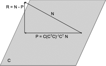
Geometric interpretation of ordinary least squares regression. A vector N (representing the PET scan of an MCI nonconverter) is projected onto a space, C, which is composed of PET scans from MCI patients who converted to AD within 2 years of being scanned. Although C is depicted as being planar, in actuality it has as many dimensions as the number of PET scan vectors that compose it. The projection vector, P, can be computed by means of multiplying a “hat” matrix by the original vector, N. The hat matrix is derived from the matrix C by the equation , where the −1 superscript represents the matrix inverse and the T superscript represents the matrix transpose. The residual vector, R, is then calculated by subtracting the projection P from N. The residual is orthogonal to all vectors in the column space of C, but retains some similarity to the original vector, N.

The goal of this project was to determine whether residual vectors computed in this manner have any utility as query vectors when used to search a database of PET scans that were not used in computation of the residual vector itself. The specific questions being posed were: (1) Do cosine similarity scores derived from the residual vectors make a significant contribution to variance in logistic regression models using AD diagnostic status or MCI conversion status as the dependent variable? (2) Can cosine similarity scores predict functional decline? (3) How do these logistic regression models fare when used as classifiers of cases not used in the model computation?

METHODS

Alzheimer's disease neuroimaging initiative (ADNI) participants

Data used in the preparation of this article were obtained from the Alzheimer's Disease Neuroimaging Initiative (ADNI) database (http://adni.loni.ucla.edu). The ADNI was launched in 2003 by the National Institute on Aging (NIA), the National Institute of Biomedical Imaging and Bioengineering (NIBIB), the Food and Drug Administration (FDA), private pharmaceutical companies, and nonprofit organizations, as a $60 million, 5-year public–private partnership. The primary goal of ADNI has been to test whether serial magnetic resonance imaging (MRI), PET, and other biological markers are useful for tracking the progression of MCI and early AD. Determination of sensitive and specific markers of very early AD progression is intended to aid researchers and clinicians to develop new treatments and monitor their effectiveness, as well as lessen the time and cost of clinical trials. The principal investigator of this initiative is Michael W. Weiner, MD, VA Medical Center and University of California, San Francisco. ADNI is the result of efforts of many coinvestigators from a broad range of academic institutions and private corporations, and subjects have been recruited from over 50 sites across the United States and Canada. The initial goal of ADNI was to recruit 800 adults, aged 55–90, to participate in the research—approximately 200 cognitively normal older individuals to be followed for 3 years, 400 people with MCI to be followed for 3 years, and 200 people with early AD to be followed for 2 years. For up-to-date information, see http://www.adni-info.org.

Participants in ADNI are assigned to a diagnostic category (cognitively normal control or NC, MCI, or AD) based on clinical evaluation. NC participants must have mini-mental state exam (MMSE) score >23, Clinical Dementia Rating (CDR) score of 0, and no exclusions or conflicting diagnoses (depression, MCI, or dementia). MCI participants must have MMSE >23, CDR = 0.5, subjective memory complaints, absence of significant impairment in nonmemory cognition or activities of daily living, and objective memory loss based on education-adjusted scores on the Wechsler Memory Scale Logical Memory II. AD participants must have MMSE score >19 and <27, CDR score of 0.5 or 1.0, and must meet NINCDS/ADRDA criteria for probable AD (McKhann et al. 1984). Of note, these criteria do not make use of MRI or PET brain imaging. The data collection procedures were approved by the institutional review board at each of the ADNI sites and all participants provided informed consent.

Anonymized data from 254 ADNI participants were acquired for this study and were classified as follows: NC (n = 79), MCI (n = 121), AD (n = 59) (see Table 1). Using subsequent determinations of conversion to AD, members of the MCI group were divided into a group of participants who converted during 2 years of follow-up (MCI-c, n = 39) and a group of participants who were followed for at least 2 years without converting (MCI-n, n = 70). The remaining 12 PET scans were excluded from further analysis due to lack of sufficient follow-up data. The final dataset comprised 242 PET scans.

Table 1.

Demographics of ADNI subjects (n = 242)

Category	Sex (M:F)ns	Age (SD)ns	MMSE (SD)*	FAQ (SD)*
Control (n = 79)	48:31	76.0 (4.8)	29.1 (0.9)	0.2 (0.7)
MCI-n (n = 70)	52:18	76.7 (7.1)	27.1 (2.6)	3.3 (4.4)
MCI-c (n = 39)	27:12	76.3 (6.9)	26.1 (2.5)	5.6 (5.1)
Alzheimer disease (n = 54)	32:22	76.1 (7.0)	22.2 (3.7)	16.0 (7.1)

^*All pairwise comparisons P < 0.05

ns = no significant difference among groups.

ADNI PET scans

Preprocessed baseline PET scans acquired with GE (Fairfield, CT), Siemens (Munich, Germany), and Philips (Amsterdam, The Netherlands) PET scanners were downloaded in ANALYZE format from the ADNI website. Preprocessing consisted of the following steps. First, six 5-min frames were identified and the last five of these frames were coregistered with the first, reducing effects of movement during the 30-min acquisition. These six coregistered frames were then averaged together and reoriented into a standard 160 × 160 × 96 voxel image grid with 1.5-mm cubic voxels. This image grid was oriented such that the anterior–posterior axis of the subject was parallel to a line connecting the anterior and posterior commissures (the AC–PC line). Scans were then intensity normalized and smoothed with a scanner-specific filter function that was determined from phantom scans acquired during the certification process. This smoothing step corrected for differences between PET scanners and produced images with a uniform isotropic resolution of 8-mm full width at half maximum (FWHM).

The downloaded scans were then spatially normalized to the SPM5 PET template (http://www.fil.ion.ucl.ac.uk/spm/). An average PET scan was generated from all of the spatially normalized scans with Automated Image Registration (AIR, Woods et al. 1998). All further PET scan processing and analysis was performed using custom software written in MATLAB® (R2007b, The MathWorks, Natick, MA). The average PET scan was used to create a mask for extraction of brain voxels. The mask was defined as all voxels with intensity >25,000. A single command in MATLAB® returns a vector containing all points at which a given comparison (e.g., >25,000) is true, ordered as if all the columns in the volume were “unwound” into a single column. This vector of points can then be used as a list of indices for a new volume, thereby selecting only the points in the new volume that correspond to the points in the mask. All mathematical procedures were then undertaken on vectors created by selecting only the voxels within the mask. Statistical analyses were performed in R (R Development Core Team, 2008), using core routines and the lme4 module for linear mixed models. Significance testing for linear mixed models made use of Markov Chain Monte Carlo permutation analysis included in the languageR module.

Projection and residual vectors

In order to create a “query” vector for the identification of similarities between any given PET scan and those of patients with AD or MCI, it was necessary to isolate those aspects of AD PET scans that differ from normal PET scans. This distinction has traditionally been made using statistical comparisons of voxels or regions of interest (ROIs). One disadvantage of the traditional approach is that it is often necessary to perform numerous comparisons, which must be statistically corrected to avoid or minimize Type I errors. The number of comparisons can be reduced by focusing the analysis on a small set of ROIs, but this approach assumes that the areas of abnormal brain tissue will correspond to the (usually) anatomically defined ROIs and that areas outside the selected ROIs are not useful for discerning among the groups. The approach described here was to locate a vector that would have low or zero cosine similarity with PET scans of members of one diagnostic group, while maintaining a relatively higher cosine similarity with the PET scans of members of another group.

The following is a description of the application of the method for discerning between subjects with AD and cognitively normal controls. Analogous methods were used for the MCI-c versus MCI-n comparisons. First, a set of AD PET scan vectors were arranged in a matrix. The projections of a group of NC scan vectors onto the column space of this matrix were then computed. As mentioned above, this process is mathematically identical to finding the least squares approximation of the solution to a system of linear equations. Each of these projections was then subtracted from the corresponding NC scan vector, yielding a set of residual vectors—one for each NC subject (Fig. 1). These residual vectors were averaged to generate a single “prototypical” residual vector. Because the average residual was a linear combination of vectors orthogonal to the AD space, the average was also certain to be orthogonal to this space. As an orthogonal vector, it had zero cosine similarity with all of the AD scan vectors. This approach is similar to using subtraction of projections to accomplish a logical NOT for search engines (Widdows and Peters 2003; Widdows 2004).

Measurements of similarity on the entire dataset were generated using the following method. The scans were first “stratified” by assigning each one to one of 10 different groups, with each group containing comparable proportions of each type of scan (i.e., because the entire sample comprised 33% NC scans, 22% AD, 16% MCI-c, 29% MCI-n, each of the 10 groups was made to approximate these proportions). Residual vectors were then computed using nine of the 10 groups and averaged together. For example, the NC scan vectors from these nine groups were projected onto the space defined by the AD scan vectors and residual vectors were obtained. The average of these residual vectors was then compared with cosine similarity to all scans in the group that was originally left out, regardless of type (i.e., diagnostic group). Thus, each scan in the left-out group received a cosine score reflecting its similarity to the residual vector obtained when AD scans were regressed out of NC scans. The process was repeated 10 times, each time leaving out one group of scans and using the remaining nine groups to create a residual vector. This method is known as stratified 10-fold cross validation.

Two sets of residual vectors were derived in this manner. The first set was derived using PET scans of cognitively normal controls and AD patients. This set consisted of two types of vectors: one created by projecting NC PET scan vectors onto a space defined by AD PET scans and one created by performing the opposite projection. The second set was derived by projecting MCI-n scan vectors onto a space defined by MCI-c PET scan vectors and then performing the opposite projection. Thus, four cosine-similarity scores were computed for each PET scan using a residual vector of each type (i.e., two from the AD/NC projections and two from the MCI-n/MCI-c projections).

Statistical analysis of measurements

Cosine similarity scores were entered individually into logistic regression models with category membership (AD vs. NC or MCI-c vs. MCI-n) as the dependent variable. Age and sex were considered as potential covariates but were removed if they failed to improve the overall fit of the model. Scores on the MMSE and Functional Activities Questionnaire (FAQ) and interactions of these scores with cosine similarity scores were considered as covariates only for the MCI-c versus MCI-n logistic regression models. MMSE and FAQ scores were not included in the AD versus NC logistic regression model due to concern of circularity, because these diagnostic classifications were assigned when subjects originally entered the study, and these scores might have influenced the classification itself. Thus, the maximal possible logistic equations were represented by Equation (1), where cosim represents the appropriate cosine similarity scores and the terms in parentheses were considered only for the MCI-c/MCI-n contrast.

(1)

Scores on the FAQ were obtained for each subject at baseline and at each follow-up visit. A linear mixed model was fitted using FAQ follow-up scores as the dependent variable, beginning with a null model and refining it by the addition of subjects as a random effect. Fixed effects were then added and those that improved the model's fit were left in. Candidate fixed effects included diagnostic group (NC, AD, MCI), baseline FAQ score, cosine similarity scores and their interactions, baseline MMSE score, and the interactions of each of these variables with time to follow-up (measured in months).

Training classifiers

The quality of the logistic regression models as classifiers was then evaluated by the following method. A logistic regression model (with the same variables that were chosen from the statistical analysis) was computed using all but one subject. Scores from the left-out subject were then entered into the logistic model to compute an output between zero and one. This output was thresholded at 11 different levels on the interval between zero and one (with increments of 0.1) to derive predictions of the subject's diagnostic or conversion status. The process was repeated for each subject, and prediction data were accumulated across all subjects. Sensitivity, specificity, and predictive value scores were calculated from the accumulated prediction data at each threshold level. Receiver operating characteristic (ROC) curves were constructed using the 11 different thresholds. The quality of the classifier at each threshold was determined by comparing it to a random classifier using McNemar's chi-square and the best classifier was selected.

Results

Statistical analysis

NC versus AD

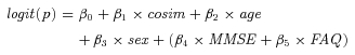
Residual vectors derived from AD and NC PET scans were used to derive cosine similarity scores for each subject. Logistic regression was used to determine the contribution of these scores to variance in odds of having AD. MCI subjects were not included in this model. Residual vectors derived by projecting AD PET scans onto NC PET scans led to the best classifier. A grand average of these residual vectors was transformed back into three-dimensional space and displayed as Fig. 2. This grand average shows that the areas of lowest residual are located in the lateral parietal and temporal regions and medial parietal/posterior cingulate regions. These areas appear grossly to correspond to the “default mode network” (Raichle et al. 2001; Greicius et al. 2004, 2008). Many of the clusters of voxels with lower residual do arise in regions considered to be within the default mode network, as can be seen in Table 2. However, some regions of high absolute residual do not clearly fit into the default mode network (e.g., the left mesial inferior occipital cluster). In addition, none of these clusters show high absolute residual in the mesial frontal regions, which figure prominently in the default mode network. Cosine similarity scores computed from these vectors made a significant contribution to the model (b = 731.9, standard error [SE] = 122.6, z = 5.97, P < 0.00001). The positive coefficient and z-score show that higher scores were associated with higher odds of having AD. Neither age nor sex improved the fit of the model and both were excluded.

Figure 2.

Grand average residual vector created by (1) projecting each AD PET scan onto a space defined by 90% of the NC PET scans, (2) subtracting the projection from the original AD PET scan to obtain a residual vector, and (3) averaging together all of the residuals. Voxels with the lowest residual values are located in the lateral temporal lobes, lateral parietal lobes, precuneus, and posterior cingulate, corresponding to the default mode network.

Table 2.

Locations of peaks in top ten areas of high residual for each contrast

	Cluster size (voxels)	Peak residual	Coordinates of peak			Anatomical description
AD versus EC	951	−3027	−62	−33	−25	Left posterior inferior temporal
	631	−2919	6	−70	44	Right precuneus
	251	−2813	−5	−102	−15	Left inferior mesial occipital
	1076	−2609	−31	−51	43	Left parietal centrum semiovale
	877	−2572	14	−51	34	Right posterior cingulate
	699	−2567	41	−54	46	Right superior parietal
	418	−2415	63	−29	−22	Right inferior temporal
	126	−2159	11	−19	13	Right thalamus
	51	−2092	−25	22	39	Left dorsolateral frontal
	109	−2067	23	71	28	Right frontal operculum
MCI-c versus MCI-n	195	2392	−16	1	72	High left dorsolateral frontal
	202	2064	−40	−62	16	Left parietal
	197	2009	−10	−70	68	High left parietal
	212	2002	26	−46	52	Right parietal centrum semiovale
	425	1756	−14	22	−28	Left orbitofrontal
	110	1668	16	−78	62	High right parietal
	48	1641	30	−16	64	Right posterior frontal
	120	1614	72	−18	−14	Right middle temporal
	112	1612	10	−78	−14	Mesial inferior occipital
	195	1609	28	−80	24	Right parietal

MCI-n versus MCI-c

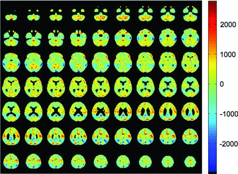
Residual vectors derived from MCI-n PET scans and MCI-c PET scans were used to derive cosine similarity scores for each subject. Logistic regression was used to determine the contribution of each of these scores to variance in odds of converting to dementia during a 2-year follow-up period. Only MCI subjects were included in this model. Residual vectors derived by projecting MCI-n PET scans onto a space defined by MCI-c PET scans resulted in cosine similarity scores with slightly better predictive power and only data related to these scores are presented here. A grand average of these residual vectors was transformed into three-dimensional space and displayed as Fig. 3. Note that these residual vectors reflect greater “normality” while those depicted in Fig. 2 reflect greater similarity to AD. Thus, in Fig. 3 it is the highest residual voxels that are located in regions that appear grossly to correspond to the default mode network. Once again, however, the top 10 clusters of high residual show only a loose correspondence with the default mode network (Table 2). The cosine similarity score made a significant contribution to the model (b = −400.1, SE = 115.8, z = −3.46, P < 0.001). The negative coefficient and z-score show that higher scores were associated with lower risk of conversion to dementia. Covariates of age and sex did not improve the fit of the model.

Figure 3.

Grand average residual vector created by the same general method as in Fig. 2, but projecting MCI-n PET scans onto a space defined by MCI-c PET scans. Voxels with the highest residual values are topographically similar to those with the low residual values in Fig. 2.

This model was enhanced somewhat by the addition of baseline FAQ score and the interaction of FAQ score with the cosine similarity score. Cosine similarity continued to make a significant contribution (b = −581.8, SE = 167.5, z = −3.48, P < 0.001). There was no main effect of FAQ score (b = −0.02, SE = 0.07, z = −0.32, P > 0.05), but the interaction of FAQ and cosine similarity was significant (b = 40.2, SE = 19.7, z = 2.04, P < 0.05).

Prediction of functional decline

All but three of the 242 subjects were entered into a linear mixed model with at least one follow-up data entry per subject (676 total observations) and the dependent variable of FAQ score at follow-up. The three excluded subjects did not have follow-up FAQ scores for the analysis. A random intercept for subject was added to an initial null model and was shown to improve the fit. Fixed effects were then added to this model. Diagnostic group and its interaction with time failed to improve the fit of the model and were not included. The strongest predictor of FAQ score at follow-up was FAQ score at baseline (b = 0.875, SE 0.03, t = 28.9, P = 0.0001). The positive t-statistic reflected a tendency for FAQ scores to trend upward with time in this population (Higher FAQ scores reflect worsening functional status). However, the interaction of FAQ score with time did not improve the model and was removed. There was a main effect of time (b = 0.074, SE 0.015, t = 4.80, P = 0.0002). There was no main effect of baseline MMSE score (b = −0.05, SE 0.1, t = −0.5, P > 0.05), but the MMSE × time interaction was negatively associated with FAQ score at follow-up (b = −0.02, SE 0.005, t = −4.68, P = 0.0002), suggesting that having a higher MMSE score at baseline was protective against functional decline. There was a main effect of cosine similarity score derived from the MCI residual vector (b = −251.2, SE 137.0, t = −1.83, P = 0.048), but no two-way interaction of this variable with time (b = −1.33, SE 6.90, t = −0.19, P > 0.05). These residual vectors were derived by projecting MCI-n PET scans onto MCI-c PET scans and would be expected to generate higher cosine similarity scores with more “normal” PET scans. The negative coefficient and t-score suggest that higher scores were associated with a lower risk of functional decline. There was no main effect of cosine similarity score derived from the AD residual vector (b = −38.7, SE 94.3, t = −0.41, P > 0.05), but this score did interact with time (b = 18.2, SE 5.2, t = 3.51, P = 0.0012). These residual vectors were derived by projecting AD PET scans onto NC PET scans and would be expected to generate higher cosine similarity scores with more abnormal PET scans. Therefore, the positive coefficient and t-score for the interaction with time suggests that higher scores are associated with greater risk of functional decline with the ongoing passage of time. The two cosine similarity scores did not interact with one another (b = 20040, SE 19420, t = 1.03, P > 0.05), but there was a three-way interaction between these scores and time (b = −2783.0, SE 1133.0, t = −2.46, P < 0.05). This finding suggests that subjects with higher AD/NC cosine similarity scores and lower MCI cosine similarity scores exhibited greater increases in FAQ over time.

Classifier accuracy

NC versus AD

The logistic regression model for discriminating between NC and AD subjects was evaluated as a classifier, using leave-one-out cross-validation. A separate model was computed with each subject left out and the ability of the model to predict the status of the subject was evaluated at 11 thresholds. Maximal sensitivity and specificity were 94.4% and 84.8%, respectively. The area under the ROC curve was 93.6% (see Fig. 4 and Table 3). The classifier performed significantly better than a random classifier (McNemar χ² = 31.3, P < 0.00001).

Figure 4.

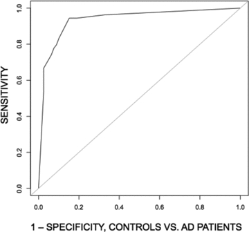
ROC curves showing performance of a simple logistic regression model for classification of subjects into elderly control and AD groups. The independent variable was a cosine similarity score computed from vectors corresponding to each subject's PET scan and residual vectors like the one depicted in Fig. 2.

Table 3.

Performance of logistic regression classifiers (“leave-one-out” cross-validation)

Comparison	AD versus controls**	MCI-c versus MCI-n*	MCI-c versus MCI-n (including FAQ)*
Sensitivity	94.4	84.6	89.7
Specificity	84.8	55.7	62.9
Positive predictive value	81.0	51.6	57.4
Negative predictive value	95.7	86.7	91.7
Area under ROC curve	93.6	72.8	76.5

^*McNemar's chi-square test versus random classifier, P < 0.05

^**P < 0.0001

MCI-n versus MCI-c

The logistic regression model predicting conversion status using only the cosine similarity score was evaluated using leave-one-out cross-validation. A separate model was computed with each subject left out and the ability of the model to predict the status of the subject was evaluated at 11 thresholds. Maximal sensitivity and specificity were 84.6% and 55.7%, respectively. The area under the ROC curve was 72.8% (see Fig. 5 and Table 3). The classifier performed significantly better than a random classifier (McNemar χ² = 5.34, P < 0.05).

Figure 5.

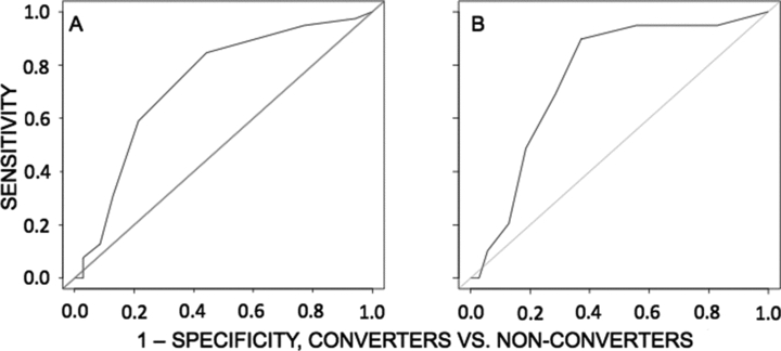
ROC curves showing performance of logistic regression models for separation of MCI subjects into a group that converted to AD within 2 years and a group that went 2 years without converting. (A) ROC curve using only cosine similarity scores for classification. These scores were derived by computing cosine similarity between each subject's PET scan and a residual vector like the one depicted in Fig. 3. (B) ROC curve using both cosine similarity scores, FAQ score, and their interaction. Addition of FAQ substantially improves the classifier.

A second classifier was evaluated, using the logistic regression model that included FAQ score and the interaction of this score with cosine similarity, again using leave-one-out cross-validation. This classifier achieved a maximal sensitivity and specificity of 89.7% and 62.9%, respectively. The area under the ROC curve was 76.5% (Fig. 5B). This classifier performed significantly better than a random classifier (McNemar χ² = 6.54, P < 0.05).

Discussion

The findings presented here constitute an initial attempt to apply fundamental concepts from IR to the AD problem set. Techniques borrowed from IR include (1) arrangement of PET scans in a vector space, with one dimension for each PET scan voxel, (2) refinement of queries by subtraction of orthogonal vectors (a technique used to implement a logical NOT operation for search engines—see Widdows 2004; Widdows and Peters 2003), and (3) scoring of PET scan “relevance” to a diagnostic query by means of cosine similarity between vectors. Cosine similarity scores derived in this manner are useful for constructing classifiers that differentiate NC subjects from AD subjects, as well as MCI patients who are destined to convert to AD within 2 years from those who are not. Furthermore, both types of cosine similarity scores derived here make independent contributions to variance in follow-up FAQ scores that supersede the contribution of diagnostic group, suggesting that this method may be useful for making more precise prognostications regarding the functional status of individuals. The validity of the method is given further support by the fact that the residual vectors bear a topographic resemblance to maps of the default mode network.

The method is computationally simple, at least relative to many techniques commonly run on modern computers. Ordinary least squares regression (the first step for computing the residual vectors) is a common approach to finding approximate solutions to many problems in statistics and engineering. Accordingly, algorithms for regression are fast and implementations are convenient. In MATLAB®, the regression step takes only one line of code and usually runs in less than 1 sec, even with large matrices. Classifiers built from structural MRI data that discern between controls and AD patients have similar accuracy to the ones presented here, but are much more computationally intensive, sometimes requiring more than 1 week to build the classifier and hours to test it (Cuingnet et al. 2010).

The method presented here compares favorably with other methods. Classifiers built from structural MRI data alone perform well when differentiating between patients with AD and subjects with normal cognition (up to 81% sensitivity with 95% specificity for voxel-based methods) (Cuingnet et al. 2010). Some studies have reported comparable accuracy with MRI methods for predicting conversion from MCI to AD, but sample sizes have been small and lack of cross-validation may mean that the results will not generalize to other samples (Convit et al. 2000). An ambitious study that compared the performance of 10 methods for building classifiers from MRI data, using cross-validation and a large sample from the ADNI database, failed to identify any method that performs better than a random classifier for discerning between MCI converters and nonconverters (Cuingnet et al. 2010). Classifiers built from FDG-PET data might perform somewhat better. For example, in a study evaluating biomarkers from the ADNI study for predicting worsening among MCI patients, glucose metabolism of the entorhinal or retrosplenial cortices were significantly correlated with change in MMSE over a 2-year period. Of the MRI measures, only retrosplenial gray matter reductions were useful for predicting change, but did so for both MMSE and CDR sum of boxes score (Walhovd et al. 2010). As a clinical tool, PET scans are useful for predicting progressive dementia, and may have sensitivity of 93% and specificity up to 76% when interpreted by an expert nuclear medicine physician (Silverman et al. 2001). However, it might be difficult to replicate these results in the absence of such an expert reader.

This work has several limitations. First, classifiers could incorporate other types of data, such as genetic testing or neuropsychological measures. Other investigators have evaluated a combination of PET and neuropsychological data for predicting changes in cognition and daily functioning, with the results suggesting that FDG-PET makes an independent contribution to such a model and might be superior to cognitive testing alone (Landau et al. 2010, 2011). One of the classifiers presented here was enhanced by the addition of FAQ score, a brief informant-based measure of daily functioning. It remains to be seen, however, whether cosine similarity scores as derived here can make an additive contribution to cognitive testing for diagnosing AD or predicting cognitive and functional decline. Future work will look to combinations of imaging measures, apolipoprotein E genotyping, and neuropsychological test scores for performing prognostications. Second, although classifiers using logistic regression have the advantage of being familiar to most clinicians, advances in machine learning (e.g., support vector machines) could add substantially to the quality of diagnoses and prognostications generated using the methods outlined here. Third, these data were acquired on a highly specific subset of patients with AD and nondementia memory impairment. Classifiers trained with these methods might not perform as well on a more heterogeneous patient population, such as the general population of patients presenting to a given memory disorders clinic, because other disease entities (vascular dementia, dementia with Lewy bodies) and other forms of nondementia cognitive impairment (executive dysfunction, progressive aphasia) may render the cosine similarity scores derived by this method less relevant. On the other hand, the method introduced here is meant to have general utility and could theoretically be adapted to apply to any of these problems.

IR is a vast and rapidly developing field with real and highly visible advances. Elementary applications of IR-like techniques like the one presented here may seed further interest in interdisciplinary work between the fields of IR and clinical neuroscience.

References

- Casey MA, Veltkamp R, Goto M, Leman M, Rhodes C, Slaney M. Content-based information retrieval: current directions and future challenges. Proc. IEEE. 2008;96:668–696. [Google Scholar]
- Chetelat G, Desgranges B, de la Sayette V, Viader F, Eustache F, Baron JC. Mild cognitive impairment: can FDG-PET predict who is to rapidly convert to Alzheimer's disease? Neurology. 2003;60:1374–1377. doi: 10.1212/01.wnl.0000055847.17752.e6. [DOI] [PubMed] [Google Scholar]
- Cuingnet R, Gerardin E, Tessieras J, Auzias G, Lehericy S, Habert M-O, et al. Automatic classification of patients with Alzheimer's disease from structural MRI: A comparison of ten methods using the ADNI database. NeuroImage. 2010;56:766–781. doi: 10.1016/j.neuroimage.2010.06.013. [DOI] [PubMed] [Google Scholar]
- Datta R, Joshi D, Li J, Wang JZ. Image retrieval: ideas, influences, and trends of the new age. ACM Comput. Surv. 2008;40:5:1–5:60. [Google Scholar]
- Drzezga A, Grimmer T, Riemenschneider M, Lautenschlager N, Siebner H, Alexopoulos P, Minoshima S, Schwaiger M, Kurz A. Prediction of individual clinical outcome in MCI by means of genetic assessment and 18F-FDG PET. J. Nucl. Med. 2005;46:1625–1632. [PubMed] [Google Scholar]
- Feldman HH, Ferris S, Winblad B, Sfikas N, Mancione L, He Y, et al. Effect of rivastigmine on delay to diagnosis of Alzheimer's disease from mild cognitive impairment: the InDDEx study. Lancet Neurol. 2007;6:501–512. doi: 10.1016/S1474-4422(07)70109-6. [DOI] [PubMed] [Google Scholar]
- Foster NL, Heidebrink JL, Clark CM, Jagust WJ, Arnold SE, Barbas NR, et al. FDG-PET improves accuracy in distinguishing frontotemporal dementia and Alzheimer's disease. Brain. 2007;130:2616–2635. doi: 10.1093/brain/awm177. [DOI] [PubMed] [Google Scholar]
- Greicius MD, Srivastava G, Reiss A, Menon V. Default-mode network activity distinguishes Alzheimer's disease from healthy aging: evidence from functional MRI. Proc. Natl. Acad. Sci. 2004;101:4637–4642. doi: 10.1073/pnas.0308627101. [DOI] [PMC free article] [PubMed] [Google Scholar]
- Greicius MD, Supekar K, Menon V, Dougherty RF. Resting-state functional connectivity reflects structural connectivity in the default mode network. Cereb. Cortex. 2008;19:72–78. doi: 10.1093/cercor/bhn059. [DOI] [PMC free article] [PubMed] [Google Scholar]
- Hebert LE, Scherr PA, Bienias JL, Bennet DA, Evans DA. Alzheimer Disease in the US population. Prevalence estimates using the 2000 census. Arch. Neurol. 2003;60:1119–1122. doi: 10.1001/archneur.60.8.1119. [DOI] [PubMed] [Google Scholar]
- Landau SM, Harvey D, Madison CM, Koeppe RA, et al. Associations between cognitive, functional, and FDG-PET measures of decline in AD and MCI. Neurobiol. Aging. 2011;32(7):1207–1218. doi: 10.1016/j.neurobiolaging.2009.07.002. [DOI] [PMC free article] [PubMed] [Google Scholar]
- Landau SM, Harvey D, Madison CM, Reiman EM. Comparing predictors of conversion and decline in mild cognitive impairment. Neurology. 2010;75:230–238. doi: 10.1212/WNL.0b013e3181e8e8b8. [DOI] [PMC free article] [PubMed] [Google Scholar]
- McKhann G, Drachman D, Folstein M, Katzman R, Price D, Stadian E. Clinical diagnosis of Alzheimer's disease: report of the NINCDS-ADRDA work group under the auspices of Department of Health and Human Services Task Force on Alzheimer's Disease. Neurology. 1984;34:939–944. doi: 10.1212/wnl.34.7.939. [DOI] [PubMed] [Google Scholar]
- Minoshima S, Frey KA, Koeppe RA, Foster NL, Kuhl DE. A diagnostic approach in Alzheimer's disease using three-dimensional stereotactic surface projections of fluorine-18-FDG PET. J. Nucl. Med. 1995;36:1238–1248. [PubMed] [Google Scholar]
- Mosconi L, Tsui WH, Pupi A, De Santi S, Drzezga A, Minoshima S, de Leon MJ. 18F-FDG PET database of longitudinally confirmed healthy elderly individuals improves detection of mild cognitive impairment and Alzheimer's disease. J. Nucl. Med. 2007;48:1129–1134. doi: 10.2967/jnumed.107.040675. [DOI] [PubMed] [Google Scholar]
- Petersen RC, Thomas RG, Grundman M, Bennett D, Doody R, Ferris S, et al. Vitamin E and donepezil for the treatment of mild cognitive impairment. New Engl J Med. 2005;352:2379–2385. doi: 10.1056/NEJMoa050151. [DOI] [PubMed] [Google Scholar]
- Raichle M, MacLeod A, Snyder A, Powers W, Gusnard D, Shulman G. A default mode for brain function. Proc. Natl. Acad. Sci. 2001;98:676–682. doi: 10.1073/pnas.98.2.676. [DOI] [PMC free article] [PubMed] [Google Scholar]
- R Development Core Team. R: a language and environment for statistical computing. Vienna, Austria: R Foundation for Statistical Computing; 2008. [Google Scholar]
- Salloway S, Ferris S, Kluger A, Goldman R, Griesing T, Kumar D, et al. Efficacy of donepezil in mild cognitive impairment. Neurology. 2004;63:651–657. doi: 10.1212/01.wnl.0000134664.80320.92. [DOI] [PubMed] [Google Scholar]
- Silverman DH, Small GW, Chang CY, Lu CS, Kung de Aburto MA, Chen W, et al. Positron emission tomography in evaluation of dementia. Regional brain metabolism and long-term outcome. J Am. Med. Assoc. 2001;286:2120–2127. doi: 10.1001/jama.286.17.2120. [DOI] [PubMed] [Google Scholar]
- Thal LJ, Ferris SH, Kirby L, Block GA, Lines CR, Yuen E, et al. A randomized, double-blind, study of rofecoxib in patients with mild cognitive impairment. Neuropsychopharmacology. 2005;30:1204–1215. doi: 10.1038/sj.npp.1300690. [DOI] [PubMed] [Google Scholar]
- Walhovd KB, Fjell AM, Brewer J, McEvoy LK. Combining MR imaging, positron-emission tomography, and CSF biomarkers in the diagnosis and prognosis of Alzheimer disease. Am. J. Neurorad. 2010;31:347–354. doi: 10.3174/ajnr.A1809. [DOI] [PMC free article] [PubMed] [Google Scholar]
- Widdows D, Peters S. Word vectors and quantum logic: experiments with negation and dysjunction. Proceedings of Mathematics of Language. 2003;8:141–154. [Google Scholar]
- Widdows D. Geometry and meaning. Stanford, CA: CSLI; 2004. [Google Scholar]
- Woods RP, Grafton S, Holmes C, Cherry S, Mazziotta JC. Automated image registration: I. General methods and intrasubject, intramodality validation. J. Comput. Assist. Tomogra. 1998;22:139–152. doi: 10.1097/00004728-199801000-00027. [DOI] [PubMed] [Google Scholar]