Berkson’s bias, selection bias, and missing data

Abstract

While Berkson’s bias is widely recognized in the epidemiologic literature, it remains underappreciated as a model of both selection bias and bias due to missing data. Simple causal diagrams and 2×2 tables illustrate how Berkson’s bias connects to collider bias and selection bias more generally, and show the strong analogies between Berksonian selection bias and bias due to missing data. In some situations, considerations of whether data are missing at random or missing not at random is less important than the causal structure of the missing-data process. While dealing with missing data always relies on strong assumptions about unobserved variables, the intuitions built with simple examples can provide a better understanding of approaches to missing data in real-world situations.

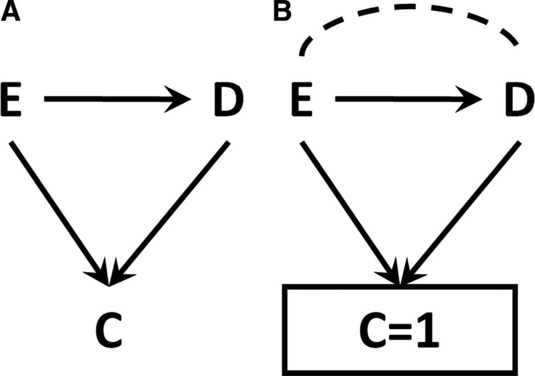
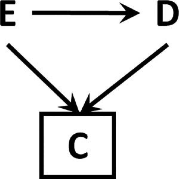
In 1946, Joseph Berkson¹ described bias in the assessment of the relationship between an exposure and a disease due to the conduct of the study in a clinic, where attendance was affected by both exposure and disease (Figure 1A)¹. Berkson observed that the fact of conducting the study in the clinic-that is, the fact of conditioning on C=1, as in Figure 1B - results in bias. Such bias – subsequently termed Berkson’s bias – can arise in prospective or retrospective studies, and in randomized or observational settings.

Figure 1. An illustration of Berkson’s Bias.

Figure 1A (left) shows a causal structure with an exposure E, an outcome D, and a factor C (clinic attendance) affected by both E and D. In Figure 1B, restricting to a level of C (C=1) leads to a non-causal association between E and D, represented with a dotted line.

While familiar in the epidemiologic literature, Berkson’s bias remains under-appreciated as a model of selection bias and, more so, of bias due to missing data. In previous work, Greenland² and Hernán et al.³ provided intuitions and insights about the structure of causal diagrams and selection bias. Here, I draw analogies between Berksonian selection bias and missing data. Like Berkson, I restrict the main discussion to a situation in which there is no confounding of the exposure-outcome relationship under study, and so consider only three variables: exposure E, disease D, and collider C.

The organization of this paper is as follows. I first remark on the structure proposed by Berkson (Figures 1A and 1B) and on close variants of that structure as a model for both selection bias and missing data bias. I then explore the four possible causal diagrams generated by the three variables (E, D, C) and the further assumption that, due to temporality, C has no causal effect on either E or D. I discuss implications of the causal structure for bias, and provide brief illustrative examples. The paper addresses additional issues in missing data, and concludes with a brief discussion.

Before proceeding, it will be useful to review the stamdard definitions of three types of missingness (missingness completely at random, at random, and not at random) as well as the definition of complete case analysis. Data are missing completely at random (MCAR), when the probability of missingness depends on values of neither observed nor unobserved data. Data are missing at random (MAR) when the probability of missingness depends only on observed data. Data are missing not at random (MNAR; alternately, there are non-ignorable missing data or non-random missingness) when the probability of missingness pattern depends (in part) on unobserved data.^4–6 A complete case analysis is one which analyzes only the non-missing data.

Berkson’s bias is a special case of collider bias

Collider bias (or collider-stratification bias, or collider-conditioning bias)^{2, 3, 7} is bias resulting from conditioning on a common effect of at least two causes. Citing Pearl,⁸ Greenland² states that if exposure E and disease D are “marginally independent (i.e., unassociated before stratification), then they will be associated within at least one stratum of a variable that they both affect.”² In terms of directed acyclic graphs (causal diagrams),⁹ E and D may be two ancestors of a common descendent C; conditioning on C leads to a distortion in the true relationship between E and D.

In Figure 1, attendance at clinic C is an effect of both exposure E and disease D. Examining the effect of E on D within a single level of C – specifically, among those attending clinic (C=1) – has the effect of introducing a non-causal association between E and D. This association is represented by a dotted line in Figure 1B.

Previous work^{2, 3} has made clear how Berkson’s bias relates to collider-stratification bias; nonetheless, two points are worth emphasizing. First, collider stratification is usually (though by no means always) explained in a situation in which exposure and disease are marginally independent; it is important to note that stratification on a collider can also introduce bias when exposure and disease are not independent. Second, while some explanations of collider bias emphasize stratification, today we understand that similar biases are introduced by any form of conditioning, including restriction and stratification on colliders.¹⁰ Berkson’s example is due to restriction to a single stratum of the collider. While an apparently minor point, this recognition gives us a key pivot for moving from selection bias to missing data. Restriction to a single level of a collider C is strongly analogous to restricting data to persons who are not missing. That is, if we consider those who did not attend clinic to be missing, then Berkson’s bias can be seen as bias introduced by a complete case analysis of (informative) missing data.

Example

Among HIV-positive women receiving antiretroviral therapy in sub-Saharan Africa, we may want to know the effect of a new pregnancy on time to AIDS. If the study is conducted at a antenatal care clinic, then both pregnancy and a new diagnosis of AIDS may affect presence at the clinic, and conduct of the study in that setting may lead to a biased estimate of the relationship between pregnancy and time to AIDS.

If neither E nor D affects C, the situation is equivalent to simple random sampling

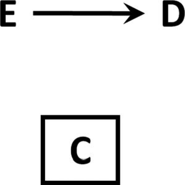
Figure 2 shows a causal structure in which neither E nor D has any causal effect on C. Thus, conditioning on C – or restricting to a level of C – is equivalent to taking a simple random sample of the original cohort. From a selection-bias perspective, this obviously will introduce no bias; from a missing-data perspective, this is equivalent to data missing completely at random.⁶

Figure 2. Causal diagram for non-informative selection bias.

Neither E nor D affects factor C, so conditioning on or restricting to a level of C amounts to simple random sampling.

This situation can be expressed as the 2×2 tables in Tables 1 and 2. Table 1 shows the hypothetical cohort of patients we would have observed if we had studied the effect of E on D in (for example) a population sampled at random from the total eligible population, (including some who attended clinic and some who did not). In Table 2 we show the study among only the proportion of patients 0 ≤ f ≤ 1 who attend clinic, where clinic attendance is not influenced by either E or D as in Figure 2.

Table 1. A 2×2 table for the effect of dichotomous exposure E on dichotomous outcome D.

	D=1	D=0	Total
E=1	A	B	A+B
E=0	C	D	C+D
Total	A+C	B+D	N

Table 2. A 2×2 table for the effect of dichotomous exposure E on dichotomous outcome D, restricting to a level of a variable C, given causal relationships shown in Figure 2.

Because C is unaffected by E or D, this is equivalent to simple random sampling; we observe a fixed proportion of individuals regardless of values of E and D (in this case, some fraction f).

	D=1	D=0	Total
E=1	fA	fB	fA+fB
E=0	fC	fD	fC+fD
Total	fA+fC	fB+fD	fN

In this case, conditioning on clinic attendance amounts to a simple random sample of size fN from the original N subjects, repeated independently for every combination of E and D. As can be readily seen in Table 2, all measures are unbiased. In this case: prevalence of exposure and outcome, risks, and contrasts of risks including risk differences, risk ratios, and odds ratios will all be unbiased after conditioning on C. Clinic attendance might be influenced by various additional factors (e.g., financial status, transportation, and so on); here we assume that those additional factors are not associated with E or D in a way that introduces bias. Independence of these additional factors and both E and D is sufficient but not necessary for lack of bias when conditioning on C.

Example

Among HIV-positive women receiving antiretroviral therapy in sub-Saharan Africa, we want to know the effect of a new pregnancy on time to AIDS. If attendance at our clinic is due only to distance of home from the clinic, (and not due to pregnancy status nor to AIDS diagnosis, directly or indirectly), then analyses of these women will be unbiased.

If E, but not D, causes C, then contrasts in risks remain unbiased in expectation

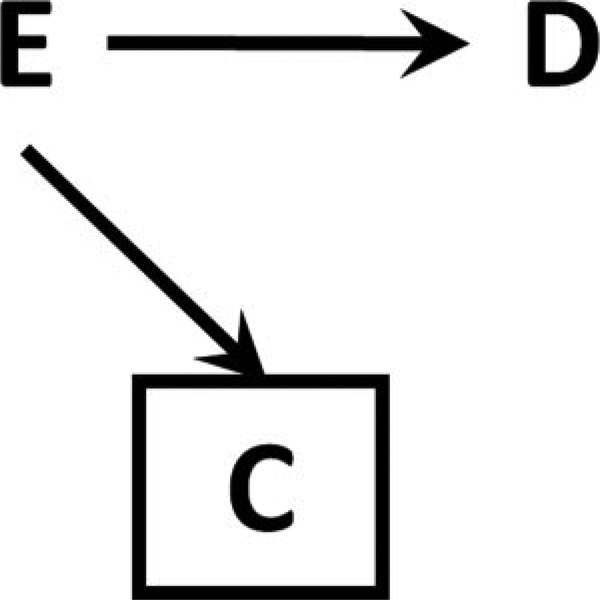
Figure 3 shows a case in which exposure E is the only cause of C. From a selection-bias perspective, restricting on C will amount to simple random sampling within level of exposure; from a missing data perspective, data are missing at random, or completely at random within level of exposure. As can be ascertained from Table 3, a crude estimate of exposure or disease prevalence will in general be biased under these conditions: for example P(D=1)= (fA+gC)/(fA + fB + gC + gD) ≠(A+C)/(A + B + C + D). However, because data are missing completely at random within exposure category, the risk by exposure status can be calculated without bias: for example, the risk P(D=1|E=1)= fA / (fA+fB) = A / (A+B), which can also be derived from Table 1. In consequence, all contrasts of risks, (including risk differences, risk ratios, and odds ratios) are unbiased in this setting.

Figure 3. Causal diagram for informative selection bias.

E, but not D, affects factor C, so conditioning on or restricting to a level of C amounts to simple random sampling within level of E.

Table 3. A 2×2 table for the effect of dichotomous exposure E on dichotomous outcome D, restricting to a level of a variable C, given causal relationships shown in Figure 3.

Because C is affected by E only, this is simple random sampling within levels of E; we observe a fixed proportion of individuals within each value of E (in this case, some fraction f when E=1, and g when E=0).

	D=1	D=0	Total
E=1	fA	fB	fA+fB
E=0	gC	gD	gC+gD
Total	fA+gC	fB+gD	fA+fB+gC+gD

This bears repeating: if exposure is the sole cause of selection into analysis or of missing data, contrasts of risks will be unbiased in a complete-case analysis. However, in real-data analysis it is almost never the case that the causal diagram is as simple as Figure 3; with more complications, it is less likely that this condition will hold. For example, if we add to Figure 3 a third variable F that causes both C and the D, C is a collider for E and F; then, conditioning on C creates bias of the E-D relationship via F (as Figure 12-5 in the book by Rothman and colleagues¹¹).

Example

Among HIV-positive women receiving antiretroviral therapy, we want to know the effect of a new pregnancy on time to AIDS. Assume our clinic does not provide extensive antenatal care beyond antiretroviral therapy, and so attendance at our clinic is lower among women after they become pregnant. If attendance is not affected by AIDS diagnosis or any other factors, then a contrast of risk of AIDS comparing pregnant and non-pregnant women attending our clinic will be unbiased.

If D, but not E, causes C, then the odds ratio (but only the odds ratio) remains unbiased in expectation

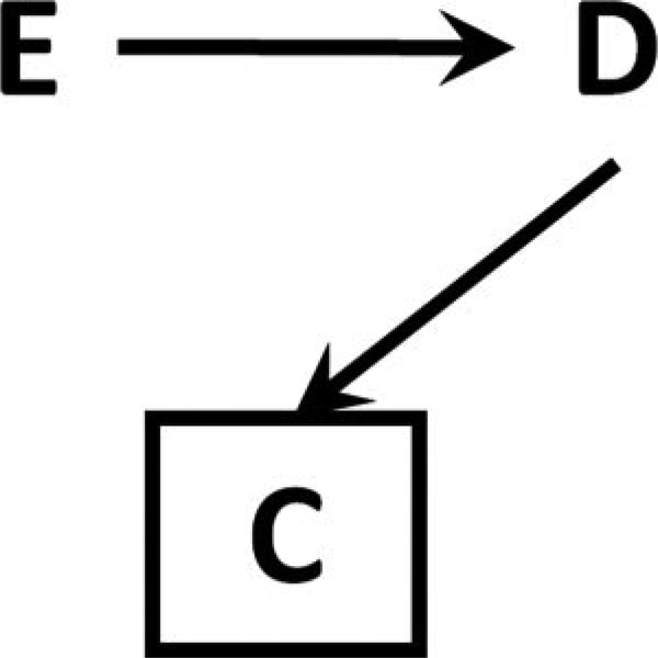
Figure 4 shows a case in which disease status D is the only cause of C. Conditioning on C leads to simple random sampling within level of the outcome (Table 4). As with Figure 3, the causal structure in Figure 4 leads to biased estimates of prevalence; but in addition, this structure leads to biased estimates of risk. In general (unless f=g), P(D=1|E=1) = fA / (fA+gB) ≠ A / (A+B).

Figure 4. Causal diagram for informative selection bias.

D, but not E, affects factor C, so conditioning on or restricting to a level of C amounts to simple random sampling within level of D.

Table 4. A 2×2 table for the effect of dichotomous exposure E on dichotomous outcome D, restricting to a level of a variable C, given causal relationships shown in Figure 4.

Because C is affected by D only, this is simple random sampling within levels of D; we observe a fixed proportion of individuals within each value of D (in this case, some fraction f when D=1, and g when D=0).

	D=1	D=0	Total
E=1	fA	gB	fA+gB
E=0	fC	gD	fC+gD
Total	fA+fC	gB+gD	fA+gB+fC+gD

Perhaps surprisingly, however, the odds ratio remains unbiased in this setting (fA gD / gB fC = AD/BC). Referring to Table 4, when f (sampling fraction among those with the outcome D=1) is equal to 1, and g < 1, then the 2×2 table is precisely analogous to a case-control study in which all cases are obtained, and controls are sampled at random from among the non-cases (a “cumulative” or “epidemic” case-control study¹¹). In such a case-control study, the case-control odds ratio provides an unbiased estimate of the cohort odds ratio; this is true in Table 4, as well. Just as in such a case-control study, we are unable to directly estimate absolute risks, risk differences, or risk ratios without additional information (e.g., f and g).¹²

Thus if outcome status is the sole direct cause of selection into a study or analysis, or of missing data, the study is analogous to a case-control study under a particular control-sampling scheme; The cohort odds ratio will be unbiased in complete case analysis – assuming no additional variables of interest as in previous examples. However, when the true effect of an exposure on the outcome is null, then missingness will not be introduced into the risk difference and risk ratio.

Example

Among HIV-positive women receiving antiretroviral therapy, we want to know the effect of a new pregnancy on time to AIDS. Assume that women are more likely to miss clinic visits if they become seriously ill, and so attendance in clinic is affected by AIDS status. If attendance at clinic is not affected by pregnancy status (or any other factors) and there is a non-null association between pregnancy and time to AIDS, then the risk difference and risk ratio for AIDS comparing pregnant and non-pregnant women will generally be biased, while an odds ratio for AIDS comparing pregnant and non-pregnant women will be generally unbiased.

If both E and D cause C, then all contrasts may be biased

Figure 5 shows classic Berkson’s bias, in which both exposure and outcome contribute to hospital attendance, and thus a different fraction may be sampled from each of the four interior cells of the 2×2 table (Table 5).^{2, 3, 11, 13} Here selection into C (or alternately, non-missing status) may be affected by both E and D and selection is at-random only within individual cells of the 2×2 table. In this case, none of the parameters-- risk difference, risk ratio, and odds ratio-- can be assumed to be unbiased in a complete case analysis except in special cases where values of f, g, h, and i make Table 5 equivalent to Table 2, 3, or 4. One critical special case is when E and D are non-interacting: when the effect of E on C is independent of the effect of D on C. In this case, Table 5 reduces to Table 4 and the odds ratio is unbiased in expectation.¹⁴

Figure 5. Causal diagram for informative selection bias.

E and D affect factor C, so conditioning on or restricting to a level of C amounts to simple random sampling within level of both E and D.

Table 5. A 2×2 table for the effect of dichotomous exposure E on dichotomous outcome D, restricting to a level of a variable C, given causal relationships shown in Figure 5.

Because C is affected by both E and D, this is simple random sampling within levels of both E and D; we observe a different proportion of individuals within each square of the 2×2 table.

	D=1	D=0	Total
E=1	fA	gB	fA+gB
E=0	hC	iD	hC+iD
Total	fA+hC	gB+iD	fA+gB+hC+iD

Example

Among HIV-positive women receiving antiretroviral therapy, we want to know the effect of a new pregnancy on time to AIDS. If attendance at our clinic rises during pregnancy and with a new AIDS-defining event, and if attendance changes synergistically with both pregnancy and AIDS together, then a contrasts of risk and odds of AIDS comparing pregnant and non-pregnant women will be generally biased.

The above comments apply whether data are missing at random or missing not at random

Recall that data are missing at random when the probability of missingness depends on observed data, and are missing not at random when probability of missingness depends at least in part on the missing data themselves.^4–6 Income data might be missing at random if age is observed for all subjects, and older people are less likely to report their income; it might be missing not at random if rich people are less likely to report their income.

Figure 3 showed a situation in which missingness is caused by exposure alone, and complete case analysis can be expected to yield unbiased risk differences, risk ratios, and odds ratios. But this figure does not specify which variable was missing as a result of the exposure. In particular, then, the discussion of Figure 3 applies whether the exposure caused missingness in the outcome (and so data are missing at random), or whether the exposure caused missingness in the exposure (and so data are missing not at random). Whether the value of the exposure led to missing outcome, or to missing exposure, missingness remains completely at random within levels of the exposure and so equivalent to simple random sampling by exposure level. Thus, even when these data are missing not at random, the complete case analysis yields unbiased estimates of the risks, risk differences, risk ratios, and odds ratios. Echoing earlier examples, pregnancy status (alone) might make it more likely that pregnancy status is missing (not at random), or that AIDS status is missing (at random): but in either case, the contrast in risk of AIDS by pregnancy status will be unbiased.

Figure 4 is also compatible with a missing-at-random condition; for example, if the value of the outcome caused the value of the exposure to be missing, then missingness would depend on observed data alone. But even when these data are missing at random, the complete case analysis yields biased estimates of the risks, the risk difference, and the risk ratio, with the odds ratio remaining unbiased. However, when data are missing at random (and models are fit correctly), both weighting¹⁵ and multiple imputation¹⁶ approaches can be used to obtain unbiased estimates of the risk difference and risk ratio. For example, AIDS status (alone) might make it more likely that pregnancy status is missing (at random), or that AIDS status is missing (not at random): in either case, a complete case estimate of the risk difference would be biased, but only in the former case would the assumptions of multiple imputation be met.

DISCUSSION

Analogies between selection bias and missing data have been made implicitly by other authors, but these analogies are not a routine part of teaching and understanding these subjects. Here, the use of simple causal diagrams has illustrated analogies between selection bias and missing data that may help to improve epidemiologists’ understanding of both subjects.

Just as others have argued with regard to selection bias^{2, 3} and overadjustment bias,^{17, 18} I here argue that structural considerations are critical for assessing the impact of missing data on estimates of effect. If the exposure is the only cause of missingness (Figure 3), then whether data are missing at random or missing not at random is largely inconsequential: in either situation, the complete case analysis is (in general) biased for prevalence, and unbiased for risks, risk differences, risk ratios, and odds ratios. If the outcome is the only cause of missingness (Figure 4), then it is likewise moot as to whether data are missing at random or missing not at random: the complete case analysis will be biased for risks, risk differences, and risk ratios, but unbiased for odds ratios. In these simple settings at least, it is the structure of the data, not whether the data are missing at random or not at random, that leads to bias in complete case analysis. Of course, in the presence of a third variable- - that is, in the majority of real world data analytic situations -- these statements require closer consideration.

Although structure is key to understanding missing data as well as selection bias, whether data are missing at random or not at random remains important because key methods for coping with missingness depend on these assumptions. Multiple imputation makes a missing-at-random assumption, for example,¹⁶ and equivalent assumptions are made for inverse-probability-of - censoring weights.¹⁵ Thus, it is not without consequence whether, for example, the unobserved value of the outcome causes missingness in the exposure or in the outcome; in the former case, multiple imputation can be applied to obtain an unbiased estimate of effect, while in the latter case multiple imputation cannot be relied upon.

Throughout this paper, I have noted that bias may be introduced by various selection mechanisms, but without attempting to quantify the bias. Bias is likely to be small when the amount of missing data is small at all levels of the exposure and disease (and in other scenarios, the covariates),¹⁴ The amount of bias observed in any real-world situation will depend on specifics (e.g., in Table 4, the relative values of f and g) which have been kept deliberately general and symbolic. As future work, it may be useful to characterize realistic values of such variables, and to attempt to estimate the amount of bias that might be introduced by such values.

Several caveats to this work should be noted. First, the situations explored here are quite simplified. The causal diagrams do not include confounders, which might occur even in a randomized setting. But as well, the causal diagrams do not include external risk factors for the outcome; this absence is essentially never the case even in a trial. This may be a particular problem if the external risk factor for the outcome is also a cause of missingness (or selection); such external factors would be a subject of future work. An additional limitation of the present discussion is that it ignores random error. Of course, I do not intend to suggest that any bias discussed here is deterministic; as in Greenland,² noted, biases correspond to asymptotic biases.² In addition, when the amount of missing data is small (again, at all levels of exposure, disease, and covariates), missing-data bias is likely to be small as well, regardless of missing-data mechanisms and causal structure.¹⁴ Finally, while selection bias and missing-data bias are closely related in the examples discussed here, the two concepts are not identical. For example, collider bias is selection bias, but need not result in missing data,^{2, 3, 7} as in the birth-weight paradox.¹⁹

Despite their simplified nature, these examples can help build intuition for the subjects at hand, and may find application in many settings. One particular setting of course is antiretroviral therapy treatment cohorts among HIV-positive individuals in sub-Saharan Africa. Vital status is a key outcome of interest in such settings, where there are high rates of loss to follow-up or drop-out^{20, 21} for which death is a relatively common reason.^{22, 23} While it may be too extreme to assume that only vital status leads to loss-to-follow-up, it may be too extreme for many applications. Vital status may sometimes be the dominant cause of loss to follow-up. This is an area where a more structural approach to missing data may be of benefit; in addition, this is a specific situation in which simulation studies might focus on quantifying the degree and amount of bias introduced by missing data.

The application of any analytic methods to missing data relies on strong assumptions about the processes that have led to missing data; if those assumptions are incorrect, then results of analysis will be misleading. In all cases, sensitivity analysis of well-defined and transparent scenarios will provide the most robust – and most responsible – inference.

REFERENCES

- 1.Berkson J. Limitations of the Application of Fourfold Table Analysis to Hospital Data. Biometrics Bulletin. 1946;2(3):47–53. [PubMed] [Google Scholar]
- 2.Greenland S. Quantifying biases in causal models: classical confounding vs collider-stratification bias. Epidemiology. 2003;14(3):300–306. [PubMed] [Google Scholar]
- 3.Hernán MA, Hernandez-Diaz S, Robins JM. A structural approach to selection bias. Epidemiology. 2004;15(5):615–625. doi: 10.1097/01.ede.0000135174.63482.43. [DOI] [PubMed] [Google Scholar]
- 4.Rubin DB. Inference and Missing Data. Biometrika. 1976;63:581–592. [Google Scholar]
- 5.Little RJA, Rubin DB. Statistical Analysis with Missing Data. New York: John Wiley; 1987. [Google Scholar]
- 6.Heitjan DF, Basu S. Distinguishing "Missing at Random" and "Missing Completely at Random". The American Statistician. 1996;50(3):207–213. [Google Scholar]
- 7.Cole SR, Platt RW, Schisterman EF, Chu H, Westreich D, Richardson D, et al. Illustrating bias due to conditioning on a collider. Int J Epidemiol. 2010;39(2):417–420. doi: 10.1093/ije/dyp334. [DOI] [PMC free article] [PubMed] [Google Scholar]
- 8.Pearl J. Causality. Second Edition. New York: Cambridge University Press; 2009. [Google Scholar]
- 9.Pearl J. Causal Diagrams for Empirical Research. Biometrika. 1995;82(4):669–688. [Google Scholar]
- 10.Porta M, editor. A Dictionary of Epidemiology. Fifth Edition. New York: Oxford University Press; 2008. [Google Scholar]
- 11.Rothman KJ, Greenland S, Lash TL. Modern Epidemiology. Third Edition. Philadelphia: Lippincott Williams & Wilkins; 2008. [Google Scholar]
- 12.Cornfield J. A method of estimating comparative rates from clinical data; applications to cancer of the lung, breast, and cervix. J Natl Cancer Inst. 1951;11(6):1269–1275. [PubMed] [Google Scholar]
- 13.Greenland S, Pearl J, Robins JM. Causal diagrams for epidemiologic research. Epidemiology. 1999;10(1):37–48. [PubMed] [Google Scholar]
- 14.Greenland S. Response and follow-up bias in cohort studies. Am J Epidemiol. 1977;106(3):184–187. doi: 10.1093/oxfordjournals.aje.a112451. [DOI] [PubMed] [Google Scholar]
- 15.Robins JM, Finkelstein DM. Correcting for noncompliance and dependent censoring in an AIDS Clinical Trial with inverse probability of censoring weighted (IPCW) log-rank tests. Biometrics. 2000;56(3):779–788. doi: 10.1111/j.0006-341x.2000.00779.x. [DOI] [PubMed] [Google Scholar]
- 16.Rubin DB. Multiple Imputation for Nonresponse in Surveys. New York: John Wiley; 1987. [Google Scholar]
- 17.Schisterman EF, Cole SR, Platt RW. Overadjustment bias and unnecessary adjustment in epidemiologic studies. Epidemiology. 2009;20(4):488–495. doi: 10.1097/EDE.0b013e3181a819a1. [DOI] [PMC free article] [PubMed] [Google Scholar]
- 18.VanderWeele TJ. On the relative nature of overadjustment and unnecessary adjustment. Epidemiology. 2009;20(4):496–499. doi: 10.1097/EDE.0b013e3181a82f12. [DOI] [PubMed] [Google Scholar]
- 19.Hernández-Díaz S, Schisterman EF, Hernán MA. The birth weight "paradox" uncovered? Am J Epidemiol. 2006;164(11):1115–1120. doi: 10.1093/aje/kwj275. [DOI] [PubMed] [Google Scholar]
- 20.Rosen S, Fox MP, Gill CJ. Patient retention in antiretroviral therapy programs in sub-Saharan Africa: a systematic review. PLoS Med. 2007;4(10):e298. doi: 10.1371/journal.pmed.0040298. [DOI] [PMC free article] [PubMed] [Google Scholar]
- 21.Sanne IM, Westreich D, Macphail AP, Rubel D, Majuba P, Van Rie A. Long term outcomes of antiretroviral therapy in a large HIV/AIDS care clinic in urban South Africa: a prospective cohort study. J Int AIDS Soc. 2009;12:38. doi: 10.1186/1758-2652-12-38. [DOI] [PMC free article] [PubMed] [Google Scholar]
- 22.Geng EH, Emenyonu N, Bwana MB, Glidden DV, Martin JN. Sampling-based approach to determining outcomes of patients lost to follow-up in antiretroviral therapy scale-up programs in Africa. Jama. 2008;300(5):506–507. doi: 10.1001/jama.300.5.506. [DOI] [PMC free article] [PubMed] [Google Scholar]
- 23.Geng EH, Bangsberg DR, Musinguzi N, Emenyonu N, Bwana MB, Yiannoutsos CT, et al. Understanding reasons for and outcomes of patients lost to follow-up in antiretroviral therapy programs in Africa through a sampling-based approach. J Acquir Immune Defic Syndr. 2010;53(3):405–411. doi: 10.1097/QAI.0b013e3181b843f0. [DOI] [PMC free article] [PubMed] [Google Scholar]