SIDEpro: a Novel Machine Learning Approach for the Fast and Accurate Prediction of Side-Chain Conformations

Abstract

Accurate protein side-chain conformation prediction is crucial for protein modeling and existing methods for the task are widely used; however, faster and more accurate methods are still required. Here we present a new machine learning approach to the problem where an energy function for each rotamer in a structure is computed additively over pairs of contacting atoms. A family of 156 neural networks indexed by amino acid and contacting atom types is used to compute these rotamer energies as a function of atomic contact distances. Although direct energy targets are not available for training, the neural networks can still be optimized by converting the energies to probabilities and optimizing these probabilities using Markov Chain Monte Carlo methods. The resulting predictor SIDEpro makes predictions by initially setting the rotamer probabilities for each residue from a backbone dependent rotamer library, then iteratively updating these probabilities using the trained neural networks. After convergences of the probabilities, the side-chains are set to the highest probability rotamer. Finally, a post-processing clash reduction step is applied to the models. SIDEpro represents a significant improvement in speed and a modest, but statistically significant, improvement in accuracy when compared to the state-of-the-art for rapid side-chain prediction method SCWRL4 on the following datasets: (1) 379 protein test set of SCWRL4; (2) 94 proteins from CASP9; (3) a set of 7 large protein-only complexes; and (4) a ribosome with and without the RNA. Using the SCWRL4 test set, SIDEpro's accuracy (χ₁ 86.14%, χ₁₊₂ 74.15%) is slightly better than SCWRL4-FRM (χ₁ 85.43%, χ₁₊₂ 73.47%) and it is 7.0 times faster. On the same test set SIDEpro is clearly more accurate than SCWRL4-RRM (χ₁ 84.15%, χ₁₊₂ 71.24%) and 2.4 times faster. Evaluation on the additional test sets yield similar accuracy results with SIDEpro being slightly more accurate than SCWRL4-FRM and clearly more accurate than SCWRL4-RRM; however, the gap in CPU time is much more significant when the methods are applied to large protein complexes. SIDEpro is part of the SCRATCH suite of predictors and available from: http://scratch.proteomics.ics.uci.edu/.

1 Introduction

Protein structure prediction is a fundamental problem in computational molecular biology and predicting the side-chain conformations for a given fixed backbone is an important subproblem [23]. Side-chain prediction methods are also critical for protein engineering, protein design, protein-protein docking [13, 1]. In both protein structure prediction and flexible protein-protein docking, the side-chain conformation predictions are relatively time intensive, and can be the limiting factor in how much search space can be explored. Thus, improvements in both speed and accuracy are highly desirable.

As a result, several methods have been proposed to address the side-chain prediction problem. SCWRL is one of the best methods and is widely used because it is generally fast and accurate, in addition it is convenient to download and run locally [5, 16]. SCWRL finds a combination of rotamers which minimizes an energy function based on rotamer probabilities and physical/chemical energy terms [5, 16]. There are two types rotamer libraries, backbone-independent and backbone-dependent. Backbone-independent rotamer libraries contain information on side-chain dihedral angles and rotamer populations. Backbone-dependent libraries contain the same information as a function of the backbone dihedral angles ø and ψ [9, 10, 8, 7]. SCWRL, and most other successful prediction methods, utilize the probabilities from backbone-dependent rotamer libraries [5, 16] and some combination of physics-based energy terms based on electrotatics, hydrogen bonding, solvation free energy [11, 18], van der Waals forces or at least simple steric energy. In addition, many search methods have been applied to the side-chain prediction problem, such as dead-end elimination [12], Monte Carlo [17, 23, 11, 18], cyclical search [25, 26], self-consistent mean field optimization [15, 20], integer programming [14], and graph decomposition [27, 16]. These methods rely on reducing the search space to pre-defined discrete sets of conformers for each side-chain (rigid rotamers) in order to make rapid predictions [1].

While physics-based energy functions have been applied with some success to the side-chain prediction problem in combination with discretized rigid rotamer models, they are not ideally suited for handling the coarseness of such models. In particular, repulsive physics-based energy terms are quite sensitive to slight changes in atom-atom distances. As a result, in the most accurate discretized models, some of the side-chains interactions inevitably have much higher repulsive energies relative to the native structures. In contrast, knowledge-based energy functions extracted from large training sets, which have been widely used in the field of protein structure prediction (e.g. [24, 28]), can be more tolerant to discretization. Furthermore, these knowledge-based energy functions can potentially capture subtle effects not captured by the physics-based approximations, and they can be trained directly on the most accurate discretized models.

Motivated by these issues, here we develop a new kind of knowledge-based energy function which is designed specifically for the rigid rotamer search space, and incorporate it into a novel side-chain prediction method, SIDEpro, which surpasses SCWRL4 in speed and accuracy. SIDEpro uses a family of artificial neural networks (ANNs) that are trained to compute an energy function based on atom-atom distances [2]. The structure models used to train the ANNs are modified versions of Protein Data Bank (PDB) structures [3], where each side-chain is independently set to the most accurate rigid rotamer. SIDEpro makes predictions by initially setting the probability of the rotamers for each residue using a backbone dependent rotamer library [9, 10, 8, 7]. Then it iteratively updates these rotamer probabilities using the ANNs energy until all the rotamer probabilities converge. Then, the side-chains are set to the rotamer with highest probability. Finally, a post-processing clash reduction procedure is applied to the models.

The remainder of the article is organized into sections covering the details of the SIDEpro methods, the results obtained for SIDEpro and SCWRL4 using several different benchmark datasets and metrics, and finally a short discussion section which summarizes the statistical significance of the results.

2 Methods

Here we present the details of the SIDEpro method in the following subsections: (1) the ANN architecture and energy function; (2) the training data and rotamer targets; (3) the full probabilistic model; (4) the Markov Chain Monte Carlo optimization procedure; (5) the fast identification of atom contacts; (6) the elimination of rotamers with backbone clashes; (7) the prediction of rotamers; (8) the clash reduction procedure; and (9) the incorporation of fixed external atoms into the prediction method. A pseudocode outline of the prediction steps is also presented in Algorithm 1.

2.1 ANN Architecture and Energy Function

At its core, SIDEpro utilizes a family of neural networks to compute an energy function. This is a computational energy function and is not necessarily meant to represent a physical quantity. Each neural network is specialized to compute a particular term of the total energy associated with a particular amino acid and the distance between a particular pair of atom types. Thus, for instance, there is a neural network for Cysteine specialized for Sulphur-Carbon distances. While we did experiment with various ANN architectures, here we report the results obtained by using a simple three layer perceptron ANN architecture, for each member of the family (Figure 1). Each ANN receives a single external input, corresponding to a distance d between a pair of atoms of the given type, and produces a single output corresponding to the “energy” of the pair. The hidden layers typically have 15-20 units. The family comprises 156 different ANNs (Table 1), indexed by three variables corresponding to: (1) the amino acid type; (2) the atom type of the first atom in the pair, restricted to side chain atoms (no backbone atoms); and (3) the atom type of the second atom in the pair, including backbone atoms. The set of atom types is {N,C,O,S,H}. When the distance between two atoms is large enough they are not considered to be interacting in our model, thus we set the energy to zero when the distance, d, is greater than 7 Å. Thus the output e of a single network can be expressed as (Figure 1):

Figure 1.

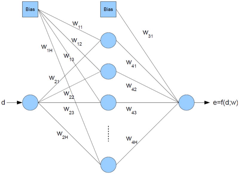
Network Architecture

Table 1.

The number of ANNs for each amino acid. Note that ALA and GLY are excluded because no side-chain search is needed for these residues. For CYS, we use two different ANNs for Sulphur-Sulphur interactions corresponding to S-S(CYS) and S-S(MET).

Amino Acid	Number of ANNs
CYS	6
ASP	10
GLU	10
PHE	5
HIS	10
ILE	5
LYS	10
LEU	5
MET	10
ASN	15
PRO	5
GLN	15
ARG	10
SER	5
THR	10
VAL	5
TRP	10
TYR	10
Total	156

$$e=f(d;w)=\{\begin{array}{ll}\sum _{h=1}^H{w}_{4h}\sigma (w_{2h}d+w_{1h})+w_{31},\hfill & d<7\hfill \\ 0,\hfill & \text{otherwise}\hfill \end{array}$$ (1)

where

• w : ANN weights

• σ : logistic sigmoid function (σ(x) = 1/(1 + e^−x))

• H : number of hidden states (15-20)

Note that a sigmoid function is not applied to the output layer because the output is not restricted to [0,1].

By adding the contributions of each neural network applied to each pair of interacting atoms it is possible to compute the total energy of each rotamer, or the total energy of a protein. In particular, the energy of rotamer j for amino acid i is calculated as follows:

$$E_{ij}=\sum _{k=1}^{N_i}\sum _{l=1,l\ne i}^L\sum _{n=1}^{N_l}{f}_{a_i{b}_{ik}{b}_{\mathit{\text{ln}}}}(||X_{\mathit{\text{ijk}}}-X_{{\mathit{\text{lr}}}_{l}n}||;\mathit{\text{w}})$$ (2)

where

• E_ij : training energy for rotamer j at residue i

• N_i : the number of atoms of residue i

• L : the length of the amino acid sequence

• X_ijk : coordinate of k-th atom of rotamer j of residue i

• a_i : amino acid type of residue i

• b_ik : atom type of k-th atom of residue i

• f_aibikbln (·) : energy term computed by the ANN associated with the amino acid type of residue i, the atom type of the k-th atom of residue i, and the atom type of the n-th atom of residue l

• r_i : rotamer target associated with residue i (see next section)

Here and in the rest of the paper we use bold-face fonts to denote vectors and contrast them with scalar variables.

A fundamental observation is that we do not have direct energy values that can be used to train the neural networks. However, we can derive rotamer targets from structures in the PDB [3]. As we shall see the energies computed by the ANNs can be converted into probabilities, and the ANNS can then be trained to maximize the probability of the target rotamers of the true structures. This optimization cannot be carried analytically but is implemented here using a Markov Chain Monte Carlo methods, essentially a variant of simulated annealing.

2.2 Training Data and Rotamer Targets

SIDEpro uses the publicly available backbone dependent rotamer library used by SCWRL3 [9][10][8][7][5] which was calculated from a set of 850 protein chains. The PISCES server was used to curate a diverse set of proteins to train the SIDEpro ANNs with the maximum mutual sequence identity set to 30%, maximum resolution of ≤ 1.8 Å, and a maximum R-factor of 20%. 2,661 proteins resulted from this search and 300 were randomly selected. Next, the 48 proteins with at least 25% sequence identity with one or protein in the SCWRL4 dataset were removed from the training set leaving 252 proteins for training.

Rather than using the raw PDB coordinates of these proteins, we set each side chain to the best matching rotamer in the corresponding rotamer library. Specifically, consider an amino acid i in a protein with R_i rotamers in the corresponding library. The library comes with a prior distribution p_ij, j = 1,…, R_i. For each one of these rotamers, there is a vector of up to four angles ${\chi }_{\mathit{\text{ij}}}=({\chi }_{ij}^k)$, k = 1,…, 4, with four corresponding normal distributions with known mean and standard deviations [7], so that: $P({\chi }_{\mathit{\text{ij}}}|{\mu }_{\mathit{\text{ij}}},{\sigma }_{\mathit{\text{ij}}})={\prod }_{k=1}^{k=4}P({\chi }_{ij}^k|{\mu }_{ij}^k,{\sigma }_{ij}^k)$. Thus for a given amino acid i in a training protein in the PDB with observed angles ${\chi }_i^{\mathit{\text{PDB}}}$, we can use Bayes theorem to compute a posterior probability for each rotamer in the corresponding family in the form:

$$P(r_{ij}|{\chi }_i^{\mathit{\text{PDB}}})=\frac{P({\chi }_i^{\mathit{\text{PDB}}}|r_{ij})p_{ij}}{P({\chi }_i^{\mathit{\text{PDB}}})}$$ (3)

Thus we assign a rotamer r_i to this amino acid by maximizing the posterior:

$$r_i=\underset{j}{\text{argmax}}P({\chi }_i^{\mathit{\text{PDB}}}|{\mu }_{\mathit{\text{ij}}},{\sigma }_{\mathit{\text{ij}}})p_{ij}$$ (4)

where ${\chi }_i^{\mathit{\text{PDB}}}$ is the vector of χ angles calculated from residue i in the native structure and p_ij is the probability of the j-th rotamer in the library for residue i.

2.3 Full Probabilistic Model

We can now proceed to use the energy computed by the ANNs to derive a full probabilistic model. The posterior probability of the training rotamer at residue i is the combination of the energy calculated by equation (2) when the weights of neural network w are given, with the rotamer library probability and is defined by:

$$P(r_i|w)=\frac{\mathit{\text{exp}}(-K{E}_{i{r}_i})p_{i{r}_i}}{{\sum }_{j=1}^{R_i}\mathit{\text{exp}}(-K{E}_{ij})p_{ij}}$$ (5)

where R_i is the number of rotamers for residue i and K is a constant (K = 0.1). We make the following standard independence approximation

$$P(r|w)={\prod }_i(r_i|w)$$ (6)

This equation can be treated as a likelihood function with the posterior distribution of w given the data r provided by Bayes theorem:

$$P(w|r)=\prod _i\frac{P(r_i|w)P(w)}{P(\mathbf{\text{r}})}$$ (7)

Here P(w) is [ the weights w of the ANNs and P(r) is a normalizing constant that does not depend on w and can be ignored during the optimization process. Each ANN has its own prior distribution, which is modeled using a set of four independent zero-mean normal distributions in the form:

$$P(w|\alpha )=\prod _{i=1}^4\sqrt{\frac{{\alpha }_i}{2\pi }}\text{exp}(-\frac{{\alpha }_i}{2}\sum _j{w}_{ij}^2)$$ (8)

where α is a vector of hyper parameters, and each component α_i controls the distribution of the corresponding weights [22, 19].

To complete the description of the full hierarchical probabilistic model, the positive hyperparameters α_i can be assumed to be independent and follow a Gamma distribution

$$P(\alpha )=\prod _{i=1}^4{\alpha }_i^{k-1}\frac{\text{exp}(-{\alpha }_i/\theta )}{{\theta }^k\Gamma (k)}$$ (9)

parameterized by k and θ. After some experimentation, we fix the value of these parameters to k = 2 and θ = 0.5.

2.4 Markov Chain Monte Carlo Optimization

To optimize the ANN weights, we use a Markov Chain Monte Carlo method [22], essentially a form of simulated annealing described, for instance, in [21]. More precisely, the idea is to use Gibbs sampling to sample from the posterior of α, and Metropolis sampling to sample from the distribution of w. By assuming r and α are independent, the posterior of w for a single ANN can be written as:

$$P(w|r,\alpha )=\frac{P(w,r,\alpha )}{P(r,\alpha )}=\frac{P(r|w,\alpha )P(w|\alpha )P(\alpha )}{P(r)P(\alpha )}=\frac{P(r|w)P(w|\alpha )}{P(r)}$$ (10)

so that:

$$P(w|r,\alpha )\propto \left(\prod _{i=1}^4\sqrt{\frac{{\alpha }_i}{2\pi }}\right)\text{exp}\left(-\sum _{i=1}^4\frac{{\alpha }_i}{2}\sum _j{w}_{ij}^2+\sum _i\text{log}P(r_i|w)\right)$$ (11)

Note that the last sum of Equation 11 ranges over all the amino acids in the training proteins where the corresponding ANN is used (e.g. for instance over all the cysteines in the set of training proteins). Similarly, for a single hyperparameter α_i associated with a specific ANN, we have

$$P({\alpha }_i|r,w)=\frac{P({\alpha }_i,r,w)}{P(r,w)}=\frac{P(r|w,{\alpha }_i)P(w|{\alpha }_i)P({\alpha }_i)}{P(r,w)}=\frac{P(r|w)P(w|{\alpha }_i)P({\alpha }_i)}{P(r,w)}$$ (12)

so that:

$$P({\alpha }_i|r,w)\propto {\alpha }_i^{k-1}\text{exp}\left(-{\alpha }_i\left({\theta }^{-1}+\frac{1}{2}\sum _j{w}_{ij}^2\right)\right)\propto \mathit{\text{Gamma}}\left(k,{\left({\theta }^{-1}+\frac{1}{2}\sum _j{w}_{ij}^2\right)}^{-1}\right)$$ (13)

Thus a Markov Chain Monte Carlo method is applied to get samples of the posterior distribution P(w, α∣r) by iteratively using:

1. Gibbs sampling for α^(j)

2. Metropolis sampling for w^(j)

Training proceeds by amino acid type, using all the ANNs associated with that particular amino acid type. For a given amino acid type and a given ANN, the learning algorithm alternates between Gibbs sampling and Metropolis sampling. Thus at the j-iteration, we first get samples of α^(j+1) by

$${\alpha }_1^{(j+1)}\sim P({\alpha }_1|{\alpha }_2^{(j)},{\alpha }_3^{(j)},{\alpha }_4^{(j)},w^{(j)})$$ (14)

$${\alpha }_2^{(j+1)}\sim P({\alpha }_2|{\alpha }_1^{(j+1)},{\alpha }_3^{(j)},{\alpha }_4^{(j)},w^{(j)})$$ (15)

$${\alpha }_3^{(j+1)}\sim P({\alpha }_3|{\alpha }_1^{(j+1)},{\alpha }_2^{(j+1)},{\alpha }_4^{(j)},w^{(j)})$$ (16)

$${\alpha }_4^{(j+1)}\sim P({\alpha }_4|{\alpha }_1^{(j+1)},{\alpha }_2^{(j+1)},{\alpha }_3^{(j+1)},w^{(j)})$$ (17)

Then we get a corresponding sample w^(j+1) by:

1. get candidate sample using

   $$\begin{array}{cc}{w}^{\ast }\sim N(w^j,{\sigma }^2)& (\text{with}\end{array}{\sigma }^2=0.1)$$ (18)

2. accept sample w* as w^(j+1) with probability $\text{min}\left[\frac{P(w^{\ast }|r,{\alpha }^{(j+1)})}{P(w^{(j)}|r,{\alpha }^{(j+1)})},1\right]$, otherwise w^(j+1) = w^(j)

The process is repeated for 500 iterations and the best observed weight w* is saved and used in prediction. The number of iterations was chosen empirically based on prediction accuracy results obtained on the training set.

$$w^{\ast }=\underset{w^{(j)}}{\text{argmax}}P(w^{(j)}|r,\alpha )$$ (19)

2.5 Fast Identification of Atom Contacts

In principle, the previous approach could require looking at all pairs of atoms in a protein in order to compute the corresponding energy term. However, most pairs of atoms are separated by a distance greater than the 7 Å cutoff and therefore are considered as non-interacting. Thus, in order to significantly reduce the calculation costs, and associated CPU time, SIDEpro identifies the spatial neighbors of each residue and then ignores all non-neighbors in the energy calculations. The corresponding pruning is implemented using simple bounding boxes: if two bounding boxes do not intersect, then the corresponding pair of atoms is separated by more than 7.0 Å and can be ignored from the energy calculation.

Neighbors are defined by checking for overlap between boxes in 3D space which are determined by subsets of residue atoms. For each residue i, a box in 3D space is calculated for the backbone atoms (3Dbox_BB(i)), the side-chain atoms allowing all rotamers (3Dbox_SC(i)), and for each rotamer j (3Dbox_Rot(i, j)). Each box is defined as the space bound by six planes. For 3Dbox_BB(i) the planes are:

$$x=\underset{k\in \mathit{\text{backbone}}(i)}{\text{min}}{X}_{i1k_x}-3.5$$ (20)

$$x=\underset{k\in \mathit{\text{backbone}}(i)}{\text{max}}{X}_{i1k_x}+3.5$$ (21)

$$y=\underset{k\in \mathit{\text{backbone}}(i)}{\text{min}}{X}_{i1k_y}-3.5$$ (22)

$$y=\underset{k\in \mathit{\text{backbone}}(i)}{\text{max}}{X}_{i1k_y}+3.5$$ (23)

$$z=\underset{k\in \mathit{\text{backbone}}(i)}{\text{min}}{X}_{i1k_z}-3.5$$ (24)

$$z=\underset{k\in \mathit{\text{backbone}}(i)}{\text{max}}{X}_{i1k_z}+3.5$$ (25)

The planes which determine 3Dbox_SC(i) are defined in the same manner, but the coordinates of all rotamers are searched:

$$x=\underset{j\in \mathit{\text{rotamers}}(i),k\in \mathit{\text{side}}-\mathit{\text{chain}}(i)}{\text{min}}{X}_{{\mathit{\text{ijk}}}_x}-3.5$$ (26)

$$x=\underset{j\in \mathit{\text{rotamers}}(i),k\in \mathit{\text{side}}-\mathit{\text{chain}}(i)}{\text{max}}{X}_{{\mathit{\text{ijk}}}_x}+3.5$$ (27)

$$y=\underset{j\in \mathit{\text{rotamers}}(i),k\in \mathit{\text{side}}-\mathit{\text{chain}}(i)}{\text{min}}{X}_{{\mathit{\text{ijk}}}_y}-3.5$$ (28)

$$y=\underset{j\in \mathit{\text{rotamers}}(i),k\in \mathit{\text{side}}-\mathit{\text{chain}}(i)}{\text{max}}{X}_{{\mathit{\text{ijk}}}_y}+3.5$$ (29)

$$z=\underset{j\in \mathit{\text{rotamers}}(i),k\in \mathit{\text{side}}-\mathit{\text{chain}}(i)}{\text{min}}{X}_{{\mathit{\text{ijk}}}_z}-3.5$$ (30)

$$z=\underset{j\in \mathit{\text{rotamers}}(i),k\in \mathit{\text{side}}-\mathit{\text{chain}}(i)}{\text{max}}{X}_{{\mathit{\text{ijk}}}_z}+3.5$$ (31)

The planes which determine 3Dbox_Rot(i, j) are defined in the same manner, but using the side-chain atoms of a specific rotamer:

$$x=\underset{k\in \mathit{\text{side}}-\mathit{\text{chain}}(i)}{\text{min}}{X}_{{\mathit{\text{ijk}}}_x}-3.5$$ (32)

$$x=\underset{k\in \mathit{\text{side}}-\mathit{\text{chain}}(i)}{\text{max}}{X}_{{\mathit{\text{ijk}}}_x}+3.5$$ (33)

$$y=\underset{k\in \mathit{\text{side}}-\mathit{\text{chain}}(i)}{\text{min}}{X}_{{\mathit{\text{ijk}}}_y}-3.5$$ (34)

$$y=\underset{k\in \mathit{\text{side}}-\mathit{\text{chain}}(i)}{\text{max}}{X}_{{\mathit{\text{ijk}}}_y}+3.5$$ (35)

$$z=\underset{k\in \mathit{\text{side}}-\mathit{\text{chain}}(i)}{\text{min}}{X}_{{\mathit{\text{ijk}}}_z}-3.5$$ (36)

$$z=\underset{k\in \mathit{\text{side}}-\mathit{\text{chain}}(i)}{\text{max}}{X}_{{\mathit{\text{ijk}}}_z}+3.5$$ (37)

Once the boxes are calculated, neighbor sets are defined for the backbone, side-chain, and each rotamer of each residue. The backbone neighbor set of residue i, Nbr_BB(i), consists of all residues l such that 3Dbox_BB(l) intersects 3Dbox_SC(i). The side-chain neighbor set, Nbr_SC(i), consists of all residues l such that 3Dbox_SC(l) intersects 3Dbox_SC(i). The rotamer neighbor set, Nbr_Rot(i, j), consists of all rotamers l, m such that 3Dbox_Rot(l, m) intersects 3Dbox_Rot(i, j). Note, however, that only the rotamers of residue-level neighbors need to be checked. This is a simple version of the approach used in SCWRL4 to construct bounding boxes for checking for clashes [16], but it is used here efficiently to avoid calculating distances for the vast majority of residue and atom pairs.

2.6 Elimination of Rotamers with Backbone Clashes

Once the residue neighbors are defined, the next step is to eliminate any rotamers which clash with the protein backbone. We define a rotamer's backbone clashing energy as:

$$E_{ij}^{\mathit{\text{VDW}}}=\sum _{k\in \mathit{\text{side}}-\mathit{\text{chain}}(i)}\sum _{l\in Nb{r}_{BB}(i)}\sum _{n\in \mathit{\text{backbone}}(l)}\{\begin{array}{ll}{(vd{w}_{ik}+vd{w}_{\mathit{\text{ln}}}-\Vert X_{\mathit{\text{ijk}}}-X_{l1n}\Vert )}^2,\hfill & \frac{\Vert X_{\mathit{\text{ijk}}}-X_{l1n}\Vert }{vd{w}_{ik}+vd{w}_{\mathit{\text{ln}}}}<0.67\hfill \\ 0,\hfill & \text{otherwise}\hfill \end{array}$$ (38)

where vdw_ik is the van der Waals radii of atom k of residue i. If E_i^VDW j > 1.0 the rotamer is considered to be clashing with the backbone and it is excluded from the search. An exception is made if all of the rotamers are clashing according to this criteria, in which case the least clashing rotamer (with lowest clashing energy) is used and all others are excluded. This approach reduces the search space significantly: on the SCWRL4 dataset approximately 20% of the rotamers are excluded from the search, resulting in a reduction of approximately 10% in average CPU time.

2.7 Prediction of Rotamers

After the rotamers which result in backbone clashes are excluded, the next step is to calculate the interaction energies between each rotamer of each residue and the entire backbone (E^BB) and the side-chains of the previously defined neighboring residues (E^SC). These interaction energies are calculated as:

$$E_{ij}^{BB}=\sum _{k\in \mathit{\text{side}}-\mathit{\text{chain}}(i)}\sum _{\text{l}\in Nb{r}_{BB}(i)}\sum _{n\in \mathit{\text{backbone}}(l)}{f}_{a_i{b}_{ik}{b}_{\mathit{\text{ln}}}}(\Vert X_{\mathit{\text{ijk}}}-X_{l1n}\Vert ;w^{\ast })$$ (39)

$$E_{\mathit{\text{ijlm}}}^{SC}=\sum _{k\in \mathit{\text{side}}-\mathit{\text{chain}}(i)}\sum _{n\in \mathit{\text{side}}-\mathit{\text{chain}}(l)}{f}_{a_i{b}_{ik}{b}_{\mathit{\text{ln}}}}(\Vert X_{\mathit{\text{ijk}}}-X_{\mathit{\text{lmn}}}\Vert ;w^{\ast })$$ (40)

where i and l represent amino acids, and j and m represent rotamers in the corresponding libraries. This decomposition is computationally efficient because the backbone is fixed and thus the backbone contribution E^BB is constant.

The probability estimates for each rotamer are initially set to the values from the rotamer library. Then, the structure-dependent energy values, E^BB and E^SC, are combined with the rotamer library probabilities to calculate the posterior probabilities for each rotamer. The predicted energy of the individual rotamers ( $E_{ij}^P$) and the corresponding probability estimates (q_ij) are the updated iteratively. Thus we first initialize the probability q_ij using the rotamer library default probabilities q_ij = p_ij and we then iterate the following two update equations:

$$E_{ij}^P=E_{ij}^{BB}+\sum _{l,m\in Nb{r}_{\mathit{\text{Rot}}}(i,j)}\mathit{\text{qlm}}{E}_{\mathit{\text{ijlm}}}^{SC}$$ (41)

$$q_{ij}=\frac{\mathit{\text{exp}}(-K{E}_{ij}^P)p_{ij}}{{\sum }_{k=1}^{R_i}\mathit{\text{exp}}(-K{E}_{ik}^P)p_{ik}}$$ (42)

SIDEpro uses only 6 iterations of this procedure, which in general is sufficient for the values to converge and yield a predicted rotamer for each residue i by setting: ${\widehat{r}}_i=\underset{j}{\text{argmax}}{q}_{ij}$.

Algorithm 1 SIDEpro Pseudocode.

Calculate boxes: 3DboxBB, 3DboxSC, and 3DboxRot

Calculate neighbor sets: NbrBB, NbrSC and NbrRot

//set qij to be pij and remove clashing rotamers

for all residue i do

for all rotamers at residue j do

qij=pij

Evdw(i, j) = calculate equation (38)

if Evdw(i, j) > 1.0 then

remove rotamer j

end if

end for

end for

//calculate EBB

for all residue i do

for all rotamers j at residue i do

EBB(i, j) = calculate equation (39)

end for

end for

//calculate ESC

for all residue i do

for all rotamers j at residue i do

for all l, m ∈ NbrRot(i, j) do

ESC(i, j, l, m) = calculate equation (40)

end for

end for

end for

// update energies and probabilities until r converges

while any qij does not converge do

for all residue i do

//update energy of rotamers at residue i

for all rotamers j at residue i do

eij = calculate equation (41)

end for

//update probability of rotamers at residue i

for all rotamers j at residue i do

qij = calculate equation (42)

end for

end for

end while

for all residue i do

${\widehat{r}}_i=\underset{j}{\text{argmax}}{q}_{ij}$

end for

where

qij : updated probability of rotamer j at residue i pij : initial probability of rotamer j at residue i (from library) r : current set of rotamers i r̂i: predicted rotamer for residue i

2.8 Clash Reduction Procedure

The initial model produced by SIDEpro uses the means of the rotamer angles, thus it can be considered to be a rigid rotamer model. When a rigid rotamer model is used, some clashes are almost always observed in a compact protein model. In fact, the structures used for training contain some clashes because the rotamers were set to the mean of the closest rotamer in the library instead of using the raw coordinates. Since the SIDEpro energy function is a computational energy function learnt from data that contains some clashes, the initial model produced by SIDEpro may contain a certain number of steric clashes. To resolve these clashes we use a post-processing method which incorporates some flexibility into the rotamers.

The clashes are minimized using the following protocol. First, each residue is checked for clashes and for those with one or more clashing atoms, the χ angles are updated to the mean (μ) ± the standard deviation (σ) multiplied by m (initially set to 0.5), then the distances between atoms are recalculated and the number of clashes are recounted. Next, the χ angles are set such that the number of clashes is minimized among the combination of μ ± σ. This operation is repeated until the clash counts converge. When the clash counts converge, the value of m is increased to 1.0 and the process is repeated. When the clash counts converge, the value of m is again increased to 1.5 and the process is repeated for the final time. This method reduces the number of clashes without a noticeable effect on accuracy.

2.9 Incorporation of Fixed External Atoms into the Prediction Method

SIDEpro can optionally incorporate fixed atoms from external molecules (other proteins, RNA, DNA, ligands, etc.) into the prediction process. These external fixed atoms are handled in a manner similar to backbone atoms. SIDEpro builds boxes and neighbors for them, and calculates the energy E_BB as if the fixed atom were backbone atoms. Since the SIDEpro ANNs are trained only on C, O, N, H and S atoms, any other atoms types are simply treated as C. In addition to handling external molecules, a subset of side-chains in the protein being predicted can be treated as fixed. These are handled by ignoring the rotamers at the fixed positions and using the input coordinates for all calculations.

3 Results

3.1 Evaluation Data and Protocol

To conduct a comparative evaluation of SIDEpro and SCWRL4, the following datasets are used: (1) the benchmark dataset of 379 proteins used to evaluate SCWRL4 [16] (SCWRL4 dataset); (2) 94 proteins determined by X-ray crystallography and released in the most recent Critical Assessment of Protein Structure Prediction Experiment (CASP9 dataset); (3) a small set of seven large protein complexes (pdb: 1RYP, 2JES, 2UVB, 3GND, 3GZU, 3K1F, 3KQK) ranging in size from 2760 to 8767 residues (COMPLEXES dataset); and (4) a ribosome (pdb: 1FJG) with and without the RNA (RIBOSOME dataset).

In SCWRL4 the default predictor utilizes a Flexibile Rotamer Model (FRM), but a Rigid Rotamer Model (RRM) is also available. The basic tradeoff between the two is that FRM is more accurate but slower than RRM [16]. Our preliminary tests of SCWRL4 confirmed this tradeoff, thus, both FRM and RRM are evaluated on each test dataset in this work and the summary results of both are compared to SIDEpro; however, only the FRM results are reported in the residue specific accuracy results for the SCWRL4 dataset (Table 3) and the CASP9 dataset (Table 5).

Table 3. SCWRL4 Dataset Residue Specific Accuracy Results.

AA Type	AA Count	χ1 (%)		χ1+2 (%)		RMSD (Å)
		SIDEpro	SCWRL4	SIDEpro	SCWRL4	SIDEpro	SCWRL4
ARG	3636	78.8	78.3	65.2	66.0	2.24	2.33
ASN	2883	85.4	83.9	61.6	59.5	1.04	1.09
ASP	4018	84.8	84.0	75.3	75.4	0.81	0.82
CYS	1001	90.4	90.3			0.48	0.47
GLN	2512	79.1	78.7	60.9	58.9	1.64	1.69
GLU	4644	73.2	72.8	57.6	56.2	1.47	1.50
HIS	1543	89.6	87.9	53.4	50.7	1.27	1.35
ILE	3968	95.6	96.0	83.4	84.7	0.45	0.43
LEU	6558	93.5	92.1	86.5	86.2	0.56	0.58
LYS	3901	79.3	76.9	66.5	63.3	1.63	1.73
MET	1410	83.8	83.8	74.5	70.3	1.14	1.27
PHE	2717	95.7	95.3	92.7	92.6	0.65	0.72
PRO	3233	83.7	85.5	80.2	81.6	0.27	0.26
SER	4107	74.0	70.8			0.73	0.80
THR	3790	90.8	90.5			0.39	0.39
TRP	979	91.6	92.1	82.6	79.5	1.16	1.37
TYR	2346	94.5	94.7	91.0	92.1	0.83	0.86
VAL	5019	93.2	93.1			0.32	0.32
Combined	58265	86.14	85.43	74.15	73.47	0.911	0.948

Table 5. CASP9 Dataset Residue Specific Accuracy Results.

AA Type	AA Count	χ1(%)		χ1+2(%)		RMSD (Å)
		SIDEpro	SCWRL4	SIDEpro	SCWRL4	SIDEpro	SCWRL4
ARG	1118	78.2	78.8	64.3	66.2	2.19	2.24
ASN	901	86.0	83.0	63.3	58.0	0.98	1.07
ASP	1396	85.9	85.5	73.1	73.6	0.81	0.81
CYS	249	89.2	90.8			0.52	0.48
GLN	756	82.7	80.0	65.5	60.3	1.51	1.64
GLU	1488	69.3	69.2	55.4	54.4	1.51	1.53
HIS	548	86.3	87.0	53.3	54.9	1.34	1.31
ILE	1341	94.6	94.6	79.6	81.4	0.53	0.51
LEU	2064	92.0	90.1	83.9	82.7	0.63	0.67
LYS	1172	78.6	77.9	64.9	63.7	1.61	1.66
MET	72	79.2	77.8	76.4	68.1	1.06	1.20
PHE	866	95.6	94.2	91.3	91.2	0.67	0.77
PRO	931	83.9	86.8	75.4	77.8	0.30	0.28
SER	1340	72.6	68.6			0.77	0.85
THR	1105	87.4	86.2			0.48	0.50
TRP	302	92.4	92.1	82.5	76.8	1.18	1.42
TYR	821	94.3	93.8	90.7	91.4	0.86	0.91
VAL	1415	89.0	89.1			0.44	0.43
Combined	17885	85.01	84.21	72.76	72.21	0.940	0.977

The summary results tables present the χ₁ accuracy, χ₁₊₂ accuracy, and RMSD averaged over all residues, the average CPU time per protein, and the total number of severe clashes and moderate clashes. The summary results are presented as follows: SCWRL4 dataset in Table 2, CASP9 dataset in Table 4, COMPLEXES dataset in Table 6, and the RIBOSOME dataset in Table 7. In all tables the best result according to each metric is shown in bold.

Table 2. SCWRL4 Dataset Summary Results: 379 Proteins, 58229 Residues.

Method	χ1(%)	χ1+2(%)	RMSD (Å)	Time (s)	Severe Clashes	Moderate Clashes
PDB					31	2048
SIDEpro	86.14	74.15	0.911	1.61	305	7227
SCWRL4-FRM	85.43	73.47	0.948	11.09	1047	9743
SCWRL4-RRM	84.15	71.24	0.995	3.84	496	6661

Table 4. CASP9 Dataset Summary Results: 94 Proteins, 17885 Residues.

Method	χ1(%)	χ1+2(%)	RMSD (Å)	Time (s)	Severe Clashes	Moderate Clashes
PDB					7	620
SIDEpro	85.01	72.76	0.940	2.06	112	2403
SCWRL4-FRM	84.21	72.21	0.977	19.06	356	3170
SCWRL4-RRM	82.83	69.79	1.030	10.64	172	2117

Table 6. COMPLEXES Dataset Summary Results: 7 Protein Complexes with 91 Chains, 30734 Residues.

Method	χ1(%)	χ1+2(%)	RMSD (Å)	Time (s)	Severe Clashes	Moderate Clashes
PDB					37	2349
SIDEpro	79.73	64.19	1.109	26.9	253	6114
SCWRL4-FRM	77.99	62.57	1.184	583.9	972	7493
SCWRL4-RRM	76.87	59.87	1.237	409.4	540	5490

Table 7. RIBOSOME Dataset Summary Results: 21 Protein Chains, 2001 Residues.

Method	χ1(%)	χ1+2(%)	RMSD (Å)	Time (s)	Severe Clashes	Moderate Clashes
Without RNA
PDB					0	370
SIDEpro	71.50	53.60	1.504	11.8	13	386
SCWRL4-FRM	70.61	52.37	1.559	180.0	54	433
SCWRL4-RRM	69.57	50.31	1.607	102.1	32	309
With RNA
SIDEpro	74.30	56.00	1.423	13.7	14	371
SCWRL4-FRM	72.31	54.49	1.480	4020.7	65	477
SCWRL4-RRM	71.46	52.81	1.524	796.2	39	340

3.2 Accuracy

Accuracy is assessed using three standard metrics: (1) percentage of side-chains where χ₁ is within 40 degrees of the experimental structure angles; (2) percentage of side-chains with both χ₁ and χ₂ within 40°; and (3) root mean square deviation (RMSD), which is calculated using the absolute coordinates of the corresponding model and experimental structure side-chain atoms. For χ₁ evaluation, the symmetries of Phe and Tyr are accounted for by calculating χ₁ using both symmetric atoms and checking each result versus the experimental structure. For χ₁₊₂ evaluation the symmetries of Asp, Phe, and Tyr are accounted for similarly. In evaluating the RMSD the symmetries of Arg, Asp, Glu, Phe, and Tyr are accounted for by calculating the RMSD using both possible atom mappings and keeping the minimum result.

The accuracy summaries calculated on the SCWRL4 dataset are presented in Table 2. Overall, SIDEpro is slightly more accurate than SCWRL4-FRM according to all three accuracy measures: χ₁ (86.14% vs 85.43%), χ₁₊₂ (74.15% vs 73.47%), and RMSD (0.911 Å vs 0.948 Å). SCWRL4-RRM is the least accurate according to all three measures. Table 3 provides the residue specific accuracy results of SIDEpro and SCWRL4-FRM on the SCWRL4 dataset [16].

The accuracy summaries calculated on the CASP9 dataset are presented in Table 4. Again, SIDEpro is slightly more accurate than SCWRL4-FRM according to all three accuracy measures: χ₁ (85.01% vs 84.21%), χ₁₊₂ (72.76% vs 72.21%), and RMSD (0.940 Å vs 0.977 Å). Again, SCWRL4-RRM is least accurate according to all three measures. Table 5 provides the residue specific accuracy results of SIDEpro and SCWRL4-FRM on for the CASP9 dataset.

The accuracy summaries calculated on the COMPLEXES dataset are presented in Table 6. On this set SIDEpro is clearly more accurate than SCWRL4-FRM according to all three accuracy measures: χ₁ (79.73% vs 77.99%), χ₁₊₂ (64.19% vs 62.57%), and RMSD (1.109 Å vs 1.184 Å). Again, SCWRL4-RRM is least accurate according to all three measures.

The accuracy summaries calculated on the RIBOSOME dataset with and without RNA are presented in Table 7. When the predictions are made without the RNA coordinates provided to the methods SIDEpro is more accurate than SCWRL4-FRM according to all three accuracy measures: χ₁ (71.50% vs 70.61%), χ₁₊₂ (53.60% vs 52.37%), and RMSD (1.504 Å vs 1.559 Å). SCWRL4-RRM is the least accurate according to all three measures. When the predictions are made in the presence of the RNA coordinates the accuracies of all three methods improve according to all three measures. SIDEpro is still the most accurate, followed by SCWRL4-FRM, with results of χ₁ (74.30% vs 72.31%), χ₁₊₂ (56.00% vs 54.49%), and RMSD (1.423 Å vs 1.480 Å). SCWRL4-RRM is still the least accurate according to the three measures.

3.3 CPU Time

Figure 2 shows the relationship between the number of residues in a protein and the prediction time for SIDEpro, SCWRL4-FRM, and SCWRL4-RRM using the 379 proteins from the SCWRL4 dataset. For SIDEpro, the time follows a predictable linear increase according to the number of residues with a Pearson correlation of 0.97. For both SCWRL methods, the time generally increases with the number of residues, but the relationship is much less predictable. The Pearson correlation for SCWRL4-RRM is 0.53 and for SCWRL4-RRM it is 0.48. On the SCWRL4 dataset the average CPU time needed by each method to make prediction is 1.61s for SIDEpro, 11.09s for SCWRL4-FRM, and 3.84s for SCWRL4-RRM (Table 2). The gap in CPU time between SIDEpro and SCWRL is more significant on the CASP9 dataset where the average CPU times are 2.06s for SIDEpro, 19.06s for SCWRL4-FRM, and 10.64s for SCWRL4-RRM (Table 4). For both of these datasets the times are calculated using all protein chains in each PDB file as input. The CPU times for all experiments are obtained using an AMD Turion 64 ×2 Mobile Technology TL-60+ at 2.00 GHz, with 3.00 GB of RAM, and running 32-bit Microsoft Windows Vista Home Premium Service Pack 2.

Figure 2.

CPU Times versus Protein Length for the 379 Protein SCWRL4 Dataset. The CPU time required by SIDEpro increases linearly with the number of residues, with a Pearson correlation of 0.97. For both SCWRL methods, the CPU time generally increases with the number of residues, but the relationships are less predictable. The Pearson correlation for SCWRL4-FRM is 0.53 and for SCWRL4-RRM it is 0.48.

For the COMPLEXES dataset the gap between the CPU times required by the different methods is much more significant. The average CPU times are 26.9s for SIDEpro, 583.9s for SCWRL4-FRM, and 409.4s for SCWRL4-FRM (Table 6). For this dataset the times are calculated using the biological assemblies as input.

On the RIBOSOME dataset without the RNA the CPU times are 11.8s for SIDEpro, 180.0s for SCWRL4-FRM, and 102.1s for SCWRL4-RRM. When the RNA coordinates are provided the CPU time for SIDEpro increases only slightly to 13.7s; in contrast the time jumps to 4020.7s for SCWRL4-FRM and 796.2s for SCWRL4-RRM (Table 7). Note that all three methods exhibit similar increases in accuracy when the RNA coordinates are utilized in prediction. In sum, once trained, SIDEpro is significantly faster than the other programs.

3.4 Clash Assessment

Two types of clashes are defined here and used for assessment: severe and moderate. In order to assess the frequency of clashes appropriately and to make fair comparisons we utilized SCWRL parameters related to steric repulsion to define clashes.

The SCWRL repulsive energy term applies no penalty if the observed distance, d, between atoms i and j is greater than the sum of their hard sphere radii (vdw_ij). The maximum penalty is applied if d/vdw_ij < .8325, and a linear ramp is used if .8235 ≤ d/vdw_ij ≤ 1 [4, 5, 16]. Thus, we define a moderate clash to occur if .8235 ≤ d/vdw_ij ≤ 1, and a severe clash if d/vdw_ij < .8325. Clashes are counted at the level of residue pairs and only the minimum observed d/vdw_ij for each residue pair is considered. This means that each residue pair can only be counted as one of: (1) unclashed, (2) moderate clash, or (3) severe clash. The radii used in this assessment are the same as those used in the SCWRL steric energy: carbon, 1.6 Å; oxygen, 1.3 Å; nitrogen, 1.3 Å; and sulfur 1.7 Å.

The counts of severe and moderate clashes observed in the models produced by SIDEpro, SCWRL4-FRM, and SCWRL4-RRM are presented in the summary tables for each dataset. The clashes observed in the corresponding PDB structures are also included for comparison. In general, the disparity in the number of clashes between the PDB structures and the models produced by all methods demonstrates that there is still room for improvement in terms of clash resolution.

On the SCWRL4 dataset the SIDEpro models have fewer severe clashes (305 vs 1047) and fewer moderate clashes (7227 vs 9743) than SCWRL4-FRM models, and also fewer severe clashes than SCWRL4-RRM models (496); however, SCWRL4-RRM has the smallest number of moderate clashes (6661).

On the CASP9 dataset the pattern is repeated. SIDEpro models have fewer severe clashes (112 vs 356) and fewer moderate clashes (2403 vs 3170) than SCWRL4-FRM models, and also fewer severe clashes than SCWRL4-RRM models (172); however, SCWRL4-RRM has the smallest number of moderate clashes (2117).

On the COMPLEXES dataset the pattern is repeated again. SIDEpro models have fewer severe clashes (253 vs 972) and fewer moderate clashes (6114 vs 7493) than SCWRL4-FRM models, and also fewer severe clashes than SCWRL4-RRM models (540); however, SCWRL4-RRM has the smallest number of moderate clashes (5490). This same pattern is also repeated on the RIBOSOME dataset both with and without RNA.

4 Discussion

Methods that can predict protein side-chains quickly and accurately can be applied in many important applications in computational molecular biology. In this investigation, we have described a new machine learning approach to the problem, resulting in a new predictor SIDEpro, and compared its performance to SCWRL4 on various datasets. In all cases, we found the same basic result: SIDEpro is more accurate and faster than both versions of SCWRL4. Table 8 summarizes the statistical significance of SIDEpro's improvements in accuracy, with respect to SCWRL4-FRM and SCWRL4-RRM, for each dataset using each metric. Considering the results on the large datasets, SCWRL4, CASP9, and COMPLEXES, the difference between SIDEpro and SCWRL4-FRM accuracies is significant at p<0.001 for all results except CASP9 χ₁₊₂ where p=0.05. When comparing SIDEpro and SCWRL4-RRM on the large datasets, all of the accuracy results presented are significant at p<1.0e-10.

Table 8. Statistical Significance (p-values) of SIDEpro Improvement with Respect to SCWRL4. Results significant at p<0.001 are shown in bold.

Dataset	AA Count	χ1	χ1+2	RMSD
SIDEpro wrt SCWRL4-FRM
SCWRL4	58265	3.1e-08	9.8e-05	<1.0e-10
CASP9	17885	7.1e-04	5.1e-02	3.4e-08
COMPLEXES	30734	<1.0e-10	1.5e-09	<1.0e-10
RIBOSOME	2001	1.7e-01	1.4e-01	1.4e-02
RIBOSOME + rna	2001	1.5e-02	9.3e-02	1.4e-02
SIDEpro wrt SCWRL4-RRM
SCWRL4	58265	<1.0e-10	<1.0e-10	<1.0e-10
CASP9	17885	<1.0e-10	<1.0e-10	<1.0e-10
COMPLEXES	30734	<1.0e-10	<1.0e-10	<1.0e-10
RIBOSOME	2001	2.1e-02	2.2e-03	2.1e-05
RIBOSOME + rna	2001	1.3e-03	3.1e-03	4.1e-05

When compared to the SCWRL4 Free Rotamer Model SIDEpro represents a moderate, but statistically significant improvement in accuracy, but the difference in CPU time is significant: SIDEpro is from 7 to 20 times faster depending on the dataset. When compared to the SCWRL4 Rigid Rotamer Model the improvement in accuracy is more significant, and SIDEpro is still from 2 to 15 times faster. In addition, SIDEpro handles proteins complexed with non-protein molecules robustly, with only a moderate increase in CPU time. Thus, SIDEpro is a useful new tool for the prediction of protein side-chains in both low- and high-throughput research projects. SIDEpro is freely available for academic use as part of the SCRATCH suite [6] available at http://scratch.proteomics.ics.uci.edu/ both as a web server and as downloadable code.

References

- 1.Andrusier Nelly, Mashiach Efrat, Nussinov Ruth, Wolfson Haim J. Principles of flexible protein-protein docking. Proteins: Structure, Function, and Bioinformatics. 2008;73(2):271–289. doi: 10.1002/prot.22170. [DOI] [PMC free article] [PubMed] [Google Scholar]
- 2.Baldi Pierre, Brunak Soren. Bioinformatics: the machine learning approach. MIT Press; 2001. [Google Scholar]
- 3.Berman HM, Battistuz T, Bhat TN, Bluhm WF, Bourne PE, Burkhardt K, Feng Z, Gilliland GL, Iype L, Jain S, Fagan P, Marvin J, Padilla D, Ravichandran V, Schneider B, Thanki N, Weissig H, Westbrook JD, Zardecki C. The protein data bank. Acta Crystallographica, Section D: Biological Crystallography. 2002;58:899–907. doi: 10.1107/s0907444902003451. [DOI] [PubMed] [Google Scholar]
- 4.Bower MJ, Cohen FE, Dunbrack RL., Jr Prediction of protein side-chain rotamers from a backbone-dependent rotamer library: A new homology modeling tool. J Mol Biol. 1997;267:1268–1282. doi: 10.1006/jmbi.1997.0926. [DOI] [PubMed] [Google Scholar]
- 5.Canutescu AA, Shelenkov AA, Dunbrack RL., Jr A graph-theory algorithm for rapid protein side-chain prediction. Protein Sci. 2003 sep;12(9):2001–2004. doi: 10.1110/ps.03154503. [DOI] [PMC free article] [PubMed] [Google Scholar]
- 6.Cheng J, Randall AZ, Sweredoski MJ, Baldi P. Scratch: a protein structure and structural feature prediction server. Nucleic Acids Res. 2005;33:W72–76. doi: 10.1093/nar/gki396. [DOI] [PMC free article] [PubMed] [Google Scholar]
- 7.Dunbrack RL., Jr Rotamer libraries in the 21st century. Curr Opin Struct Biol. 2002;12:431–440. doi: 10.1016/s0959-440x(02)00344-5. [DOI] [PubMed] [Google Scholar]
- 8.Dunbrack RL, Jr, Cohen FE. Bayesian statistical analysis of protein sidechain rotamer preferences. Protein Sci. 1997;6:1661–1681. doi: 10.1002/pro.5560060807. [DOI] [PMC free article] [PubMed] [Google Scholar]
- 9.Dunbrack RL, Jr, Karplus M. Backbone-dependent rotamer library for proteins: Application to side-chain prediction. J Mol Biol. 1993;230:543–574. doi: 10.1006/jmbi.1993.1170. [DOI] [PubMed] [Google Scholar]
- 10.Dunbrack RL, Jr, Karplus M. Conformational analysis of the backbone-dependent rotamer preferences of protein sidechains. Nat Struct Biol. 1994;1:334–340. doi: 10.1038/nsb0594-334. [DOI] [PubMed] [Google Scholar]
- 11.Eyal Eran, Najmanovich Rafael, Mcconkey Brendan J, Edelman Marvin, Sobolev Vladimir. Importance of solvent accessibility and contact surfaces in modeling side-chain conformations in proteins. Journal of Computational Chemistry. 2004;25(5):712–724. doi: 10.1002/jcc.10420. [DOI] [PubMed] [Google Scholar]
- 12.Goldstein RF. Efficient rotamer elimination applied to protein side-chains and related spin glasses. Biophys J. 1994;66:1335–1340. doi: 10.1016/S0006-3495(94)80923-3. [DOI] [PMC free article] [PubMed] [Google Scholar]
- 13.Gray Jeffrey J, Moughon Stewart, Wang Chu, Schueler-Furman Ora, Kuhlman Brian, Rohl Carol A, Baker David. Protein-protein docking with simultaneous optimization of rigid-body displacement and side-chain conformations. Journal of Molecular Biology. 2003;331(1):281–299. doi: 10.1016/s0022-2836(03)00670-3. [DOI] [PubMed] [Google Scholar]
- 14.Kingsford CL, Chazelle B, Singh M. Solving and analyzing side-chain positioning problems using linear and integer programming. Bioinformatics. 2005;21:1028–1036. doi: 10.1093/bioinformatics/bti144. [DOI] [PubMed] [Google Scholar]
- 15.Koehl P, Delarue M. Application of a self-consistent mean field theory to predict protein side-chains conformation and estimate their conformational entropy. J Mol Biol. 1994;239:249–275. doi: 10.1006/jmbi.1994.1366. [DOI] [PubMed] [Google Scholar]
- 16.Krivov GG, Shapovalov MV, Dunbrack RL., Jr Improved prediction of protein side-chain conformations with scwrl4. Protein. 2009 dec;77(4):778–95. doi: 10.1002/prot.22488. [DOI] [PMC free article] [PubMed] [Google Scholar]
- 17.Liang S, Grishin NV. Side-chain modeling with an optimized scoring function. Protein Sci. 2002;11:322–331. doi: 10.1110/ps.24902. [DOI] [PMC free article] [PubMed] [Google Scholar]
- 18.Lu Mingyang, Dousis Athanasios D, Ma Jianpeng. Opus-rota: A fast and accurate method for side-chain modeling. Protein Science. 2008;17(9):1576–1585. doi: 10.1110/ps.035022.108. [DOI] [PMC free article] [PubMed] [Google Scholar]
- 19.MacKay DJC. ASHRAE Transactions. Pt.2. Vol. 100. ASHRAE; 1994. Bayesian non-linear modelling for the prediction competition; pp. 1053–1062. [Google Scholar]
- 20.Mendes Joaquim, Soares Cl̃aąudio M, Carrondo Maria Arm̃l'nia. Improvement of side-chain modeling in proteins with the self-consistent mean field theory method based on an analysis of the factors influencing prediction. Biopolymers. 1999;50(2):111–131. doi: 10.1002/(SICI)1097-0282(199908)50:2<111::AID-BIP1>3.0.CO;2-N. [DOI] [PubMed] [Google Scholar]
- 21.Muramatsu D, Kondo M, Sasaki M, Tachibana S, Matsumoto T. A markov chain monte carlo algorithm for bayesian dynamic signature verification. IEEE T Inf Foren Sec. 2006;1:22–34. [Google Scholar]
- 22.Neal RM. Bayesian Learning for Neural Networks. Springer-Verlag; 1996. [Google Scholar]
- 23.Rohl Carol A, Strauss Charlie EM, Chivian D, Baker D. Modeling structurally variable regions in homologous proteins with rosetta. Proteins. 2004;55:656–677. doi: 10.1002/prot.10629. [DOI] [PubMed] [Google Scholar]
- 24.Simons K, Ruczinski I, Kooperberg C, Fox BA, Bystroff C, Baker D. Improved recognition of native-like protein structures using a combination of sequence-dependent and sequence-independent features of proteins. Proteins. 1999;34:82–95. doi: 10.1002/(sici)1097-0134(19990101)34:1<82::aid-prot7>3.0.co;2-a. [DOI] [PubMed] [Google Scholar]
- 25.Xiang Z, Honig B. Extending the accuracy limits of prediction for side-chain conformations. J Mol Biol. 2001;311:421–430. doi: 10.1006/jmbi.2001.4865. [DOI] [PubMed] [Google Scholar]
- 26.Xiang Zhexin, Steinbach Peter J, Jacobson Matthew P, Friesner Richard A, Honig Barry. Prediction of side-chain conformations on protein surfaces. Proteins: Structure, Function, and Bioinformatics. 2007;66(4):814–823. doi: 10.1002/prot.21099. [DOI] [PMC free article] [PubMed] [Google Scholar]
- 27.Xu Jinbo. Rapid protein side-chain packing via tree decomposition. In: Miyano Satoru, Mesirov Jill, Kasif Simon, Istrail Sorin, Pevzner Pavel, Waterman Michael., editors. Research in Computational Molecular Biology, volume 3500 of Lecture Notes in Computer Science. Springer; Berlin/Heidelberg: 2005. pp. 423–439. [DOI] [Google Scholar]
- 28.Zhang Y, Kolinski A, Skolnick J. Touchstone:ii a new approach to ab initio protein structure prediction. Biophys J. 2003;85:1145–1164. doi: 10.1016/S0006-3495(03)74551-2. [DOI] [PMC free article] [PubMed] [Google Scholar]