How local is the local field potential?

Summary

Local field potentials (LFPs) are of growing importance in neurophysiological investigations. LFPs supplement action potential recordings by indexing activity relevant to EEG, MEG and hemodynamic (fMRI) signals. Recent reports suggest that LFPs reflect activity within very small domains of several hundred microns. We examined this conclusion by comparing LFP, current source density (CSD), and multiunit activity (MUA) signals in macaque auditory cortex. Estimated by frequency tuning bandwidths, these signals' “listening areas” differ systematically with an order of: MUA < CSD < LFP. Computational analyses confirm that observed LFPs receive non-local contributions. Direct measurements indicate passive spread of LFPs to sites more than a centimeter from their origins. These findings appear to be independent of the frequency content of the LFP. Our results challenge the idea that LFP recordings typically integrate over extremely circumscribed local domains. Rather, LFPs appear as a mixture of local potentials with “volume conducted” potentials from distant sites.

Introduction

Broad band neuroelectric field potentials recorded from within the brain have been used to investigate brain functioning in nonhuman animals began shortly after the discovery of the electroencephalogram or EEG (Bullock, 1945;Galambos, 1941;Marshall et al., 1937). While the technique was overshadowed by action potential recording for a number of years, its importance has re-emerged over the past decade because of the observations that the field potential is linked to the neural underpinnings of hemodynamic signals (Logothetis et al., 2001), as well as magnetoencephalographic (MEG) and scalp EEG signals (Heitz et al., 2010;Mitzdorf, 1985;Schroeder et al., 1991; Steinschneider et al., 1992). Additionally, it is now widely recognized [e.g., (Schroeder et al., 1998)] that because field potentials are generated by transmembrane current flow in ensembles of neurons (Eccles, 1951; Lorente de No, 1947), they can index processes and events that are causal to action potentials. Finally, field potentials form part of the signal spectrum that can drive neuro-prosthetic devices (Hatsopoulos and Donoghue, 2009), even when accessed indirectly with noninvasive recording from the scalp (Wolpaw, 2007).

Recent reports have suggested that field potentials recorded within the brain are in general, extremely local phenomena, reflecting neuronal processes occurring within approximately 200–400 μm of the recording electrode in the cortex (Katzner et al., 2009;Xing et al., 2009). This basic proposition is imbued in the common use of the term local field potential (LFP), which has become widespread in the literature, particularly over the last 10 years. However, the proposition seems at odds with many prior studies, which suggest that LFPs spread laterally over distances of 600~1000 μm (Berens et al., 2008), 2–3 mm (Nauhaus et al., 2009; Wang et al., 2005), 5 mm (Kreiman et al., 2006), and vertically over centimeter scales (Schroeder et al., 1992). Importantly, reports emphasizing the extreme local origins of the LFP (Katzner et al., 2009;Xing et al., 2009) have been largely confined to visual cortices on the brain surface, and have analyzed the spread of LFPs only in the “lateral” dimension. This is but one of the relevant dimensions that need to be considered, especially given that models of the underlying generators of scalp ERP/EEG components often contain directional terms (Ingber and Nunez, 2011;Srinivasan et al., 2006;Winter et al., 2007). Spread of LFPs along 'vertical' dimensions creates apparent similarity and coherence between depths (Maier et al., 2010), though it could be just due to the volume conduction (Kocsis et al., 1999). To provide a more general assessment of the spatial spread of LFPs, we examined the issue in the context of tonotopic mapping in primary auditory cortex (A1). Corresponding to the precise mapping of the retinal receptor surface in V1 as examined by recent studies (Katzner et al., 2009;Xing et al., 2009), A1 contains a precise spatial map of the cochlear surface (Kosaki et al., 1997;Merzenich and Brugge, 1973), which allows examination of the lateral spread of LFPs as was done in V1. Moreover, due to A1's placement in the inferior bank of the lateral sulcus, vertical penetrations through A1 could examine the spatial spread of LFPs in the vertical dimension as well.

A central concern in LFP analysis is that with use of distant, extracranial reference electrodes, there is uncertainty as to the precise neural generator of the LFP, which is in part why the first and second spatial derivatives of the LFP were explored as additional measures (Mitzdorf, 1985). The second derivative of the LFP, known as current source density (CSD) also estimates the net local pattern of neuronal transmembrane current flows that generate an LFP distribution in the extracellular medium (Nicholson, 1973;Nicholson and Freeman, 1975), and is a centerpiece of our analysis. We directly compared the vertical and lateral spread of the LFP recorded with a distant reference, with that of the derived CSD signal and that of the concomitant multiunit activity (MUA) signal. LFP and MUA signals were sampled with linear array multielectrodes (100 or 200 μm spacing) placed in and near A1 in awake monkeys.

Our findings clearly indicate lateral spread of the LFP well beyond the 200~400 μm range, with a vertical spread also extending many millimeters beyond auditory cortex. These findings challenge the notion that LFPs can be generally assumed to represent very local neuronal processes. They emphasize the critical importance of considering technical factors such as reference electrode location, as well as physiological factors such as the spatial extent/configuration and activation strength/symmetry of the underlying neuronal generators, in the interpretation of LFP recordings.

Results

Data were collected from awake monkeys that were conditioned to sit quietly in the primate chair and accept painless head restraint, but were not required to attend or respond to the auditory stimuli. A1 yields robust and consistent responses to suprathreshold tones under these conditions (O'Connell et al., 2011;Steinschneider et al., 2008), comparable in quality to those generated by attended auditory stimuli (Lakatos et al., 2009). Laminar profiles of auditory-evoked LFPs and MUA were recorded with linear array multielectrodes (100 or 200 μm inter-contact spacing) positioned for each experiment so that they straddled the layers of A1. To illustrate the recording preparation and methods, Figure 1 depicts averaged laminar profiles of response to the “best frequency” (BF) tone of one penetration site in A1 (see methods for details on BF determination). Laminar LFP profiles are shown in both raw, line plot (A) and in a more intuitive color plot (B) formats, both of which are used in subsequent figures. On the right (C) is the CSD profile derived from the LFP profile, with selected MUA recordings superimposed to help connect current source and sink configurations with local physiological processes. Layers are identified functionally using standard criteria; e.g., the initial current sink and largest peak MUA in response to robust sensory input occurs in Layer 4 (Lakatos et al., 2007;Schroeder et al., 2001;Steinschneider et al., 1992).

Figure 1. Laminar patterns of auditory responses of LFP, CSD and MUA in the auditory cortex.

Responses to the BF tone in one example A1 site. Line plots (A) show LFP responses recorded at 23 depths using a linear array multielectrode with 100 μm intercontact spacing (schematic on left). In center (B) is the color plots of the laminar LFP profile shown in A; with negative deflection colored red and positive deflections colored blue. (C) depicts the CSD profile derived by the second derivative approximation of the field potential profile in A and B; red depicts extracellular current sinks (associated with net local inward transmembrane current flow) and blue depicts extracellular current sources (associated with net local outward transmembrane current flow). Selected MUA responses from channels 2, 6, 10, 15, and 19 are superimposed on the CSD plot. Vertical thin lines in all columns indicate stimulus onset. In this example, the peak of MUA at channel 15 corresponded to the peak negativity of LFP and current sink (CSD) at the response onset in Layer 4, and the responses from this location were used for analyzing lateral spread of signals. The asterisk indicates a superficial sink that produced N50.

These data illustrate the local cortical ensemble response to a suprathreshold (60 dB), 100 ms duration tone at the penetration site's preferred frequency. Response onset consists of an initial current sink with a robust concomitant increase in MUA in Layer 4, followed by subsequent CSD responses accompanied by less marked MUA in the supra and infragranular layers. The form of the excitatory response, initial transient with a lesser sustained component is one of the common variant tone responses observed in A1 [e.g., (O'Connell et al., 2011)]. The initial activation of Layer 4 is reflected in an LFP negativity that arises in association with the collocated current sink (“1” in Fig. 1 B, C), and with a current sink that begins slightly later in Layer 3 (“2” in Fig. 1 B, C). It is sometimes possible, as in this case, to discern an earlier negativity that arises in association with a sink/source configuration and a brief MUA burst below layer 4 (“-1” in Fig. 1 C). Modeling and physiology experiments suggest that the initial transient responses in primary sensory cortices are a combination of presynaptic (afferent terminal discharge), and postsynaptic (granule cell depolarization) processes (Schroeder et al., 1995;Steinschneider et al., 1992;Tenke et al., 1993). In most cases the presynaptic component is masked by a much larger postsynaptic component.

The larger, more obvious LFP, the positivity peaking at ~30 ms, and the negativity peaking at ~50 ms (P30/N50, Fig. 1 A, B, and C) appear to arise mainly from processes in the supragranular layers. The superficial P30 extends upwards from a supragranular current source that we interpret as a “passive” CSD feature reflecting current return to the “active” current source, itself representing the initial activation of supragranular pyramidal cells (by granule cell afferents from Layer 4). Passive current return happens because of the conservation of net electrical currents and electrical neutrality. N50 extends vertically from a superficial current sink (an asterisk in Fig. 1C), whose physiological significance is less clear. As discussed below, we use the P30 to track LFP spread vertically. To get at lateral spread of LFPs, we focused analysis on the initial negativity associated with the frequency-selective responses in Layer 4/lower Layer 3 (“1” and “2” Fig. 1); this negativity extends in a ventral direction from the current sinks in these locations, particularly the lower (Layer 4) one. Figure 2 shows Layer 4 MUA, CSD and LFP responses to tones in two different A1 penetration sites. In each site, it is clear that the three signals were largest in response to same tone frequencies, and thus shared a common BF. However, while MUA and CSD responses to tones disappeared as the tone frequency moved away from the BF, the LFP response did not.

Figure 2. Time courses of responses to tones.

Tone-evoked MUA, CSD and LFP responses at two example sites (A and B). MUA, CSD and LFP responses are colored blue, green and red, respectively. All time-bases extend from −30 to 170 ms relative to the onset of 100 ms duration tones, whose onsets and offsets are indicated by vertical dotted lines. Tone frequencies are indicated on the top row (kHz).

Tuning curves were derived by measuring mean response amplitudes over 10 ms periods, centered between 23 and 30 ms following the stimulus onset at a recording depth within the Layer 4 (see methods). The mean amplitude of MUA, CSD and LFP signals indicated change in the level of local neuronal firing, the magnitude of current sinks due to excitatory synaptic currents and the magnitude of LFP negativity caused by current sinks relative to the baseline levels, respectively. The period was chosen to be the time during both LFP and CSD signals were negatively deflected along with simultaneous increase in MUA. Figure 3A and B show the normalized tuning curves for LFP, CSD and MUA signals in the two example cases shown in Fig. 2A and B, respectively. The three types of tuning curve generally peak at the same tone frequencies. The same trend was observed across all recording sites (Fig. 3C). BF estimates were not significantly different between the 3 signals (Friedman's non-parametric repeated measures ANOVA, χ_γ² (2, n=130) = 0.92, p = 0.2, Fig. S1). The tuning bandwidths of MUA, CSD and LFP differed significantly from one another (Friedman's non-parametric repeated measures ANOVA, χ_γ² (2, n=130) = 85.2, p < 0.01), in an order of BW_MUA < BW_CSD < BW_LFP (Tukey's HSD test, all comparisons p < 0.05, Fig. 3D). Similar results were found for the tuning of 3 signals in the supragranular layers (Fig. S2), where BW_MUA did not differ significantly from layer 4 (Wilcoxon rank sum test, p = 0.34). Two physiological factors likely can account for these differences. First, due to reflection of subthreshold synaptic currents in the CSD measure, the tuning of CSD responses to tones is wider than that of MUA responses to the same tones. Second, due to volume conduction of electrical events in auditory cortical loci tonotopically not matched to the penetration sites, the tuning of LFP is wider than that of CSD measures.

Figure 3. Normalized tuning curves for MUA, CSD and LFP.

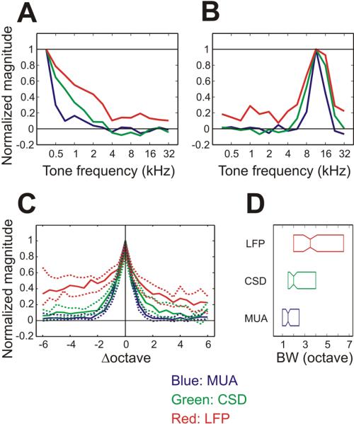
(A and B) tuning curves of two exemplars shown in Figure 2. Colors of curves correspond to MUA (blue), CSD (green) and LFP (red). (C) Summary of tuning curves across all penetration sites. Line and dotted line traces represent the median and its 95% confidence intervals of all recording sites (n=130). The MUA, CSD and LFP tuning curves of the individual sites were shifted on the frequency axis to align the best frequencies of MUA tuning curves on zero. (D) Boxplot showing the median and the first and third quartiles of BW_MUA (blue), BW_CSD (green) and BW_LFP (red).

The idea that LFP responses to tones octaves away from the BF at a penetration site in A1 is due to volume conduction, predicts that the CSD index derived by numeric differentiation from such an LFP profile should not contain the “volume conducted” components. In other words, the local spatiotemporal distribution of sources and sinks outlined by CSD analysis would not be able to generate the observed profile of LFP response (LFP_obs). To test this idea, laminar LFP responses (LFP_cal) were calculated back from CSD profiles. According to Poisson's differential equation, the local LFP profile is the spatial integration of its solution given a particular spatial distribution of current sinks/sources identified by CSD analysis (methods).

Figure 4A (left column) shows laminar-temporal profiles of LFP_obs responses to tones, in a penetration site tuned toward low frequencies. The profiles maintained common patterns across tone frequencies: the predominant onset negativity in the bottom two thirds of channels and positivity in the top one third of channels across tone frequencies. Other later features, like the strong positivity around 50 ms in the bottom of the profile, were preserved only for responses to lower frequency tones. CSD responses (Fig. 4A, second column) are similar to LFP_obs in terms of their strength across frequencies below 1.4 kHz. However, CSD responses are nearly abolished at high stimulus frequencies. Tuning curves in Figure 4B also show that CSD responses were nearly zero at high stimulus frequencies where LFP_obs responses still had amplitudes about 20% of peak values. Figure 4A (third column) shows laminar-temporal profiles of LFP_cal derived from CSD profiles using Equation 1 (methods). Note that our simultaneous recording from single arrays orthogonal to cortical layers cannot resolve the fine details of spatial distributions for sinks/sources. For example, lateral spread of activity may differ between layers, but cannot be elucidated by our methods. Regardless, application of Eq. 1 to CSD worked qualitatively well to calculate LFP when that was generated locally. LFP_cal at low frequencies had largely similar profiles to LFP_obs from the onset to the later inversions of polarity across similar subsets of the recording depths. As the tone frequency increased, the response became weaker. At high stimulus frequencies where CSD responses were negligible, the LFP_cal diverged markedly from the LFP_obs and more portions of signals differed in their sign (Fig. 4A fourth column).

Figure 4. Comparisons of LFP_obs and LFP_cal.

(A) Laminar-temporal profiles (−30 – 170 ms) of LFP_obs, CSD, LFP_cal responses, and disparity of signs between LFP_obs and LFP_cal (from left to right) responses to tones of frequencies from 0.35 kHz (top) to 32 kHz (bottom) of one example recording site. In the first to third columns, red and blue correspond to negative and positive polarities, respectively. In the forth column, red indicates positions of unequal polarity (Δsign) between laminar-temporal profiles of LFP_obs and LFP_cal responses. White vertical lines indicate the onset and offset of tones. (B) Tuning curves (blue: MUA, green: CSD, red: LFP_obs) of the example site shown in A, with SX_Corr (black) overlain over tone frequencies (see text for details). (C) Summary of S_XCorr curves across penetration sites. Line and dotted line curves represent the median and its 95% confidence intervals estimated from all penetration sites (n=130).

We calculated S_XCorr that quantified how well the shape of LFP_cal matched to that of LFP_obs, irrespective of difference in response magnitudes between the two LFP profiles for individual tone frequencies. For the example shown in Figure 4A, S_XCorr peaked at 1 kHz the frequency at which the amplitude of LFP_obs response also peaked (Fig. 4B). Up to 2.8 kHz, the S_XCorr was above 0.8 and but it fell off at higher frequencies. Across all recording sites, S_XCorr gradually decreased as the tone frequency departed from the BF_MUA (Fig. 4C). At frequencies beyond 1 octave difference, median S_XCorr were significantly different from that at BF_MUA (bootstrap, two-tailed, P<0.05).

These results can be explained by volume conduction. Tones at BF_MUA evoke strong MUA and CSD responses (Fig. 3C). CSD responses accompanied with MUA more likely reflect local activity than CSD responses without MUA concomitants (e.g. near the foot of tuning curve), and these are strong enough to generate similarly strong (and local) LFP responses like those to low frequency tones shown in Figure 4A. Tones that are away from the BF_MUA may still evoke weaker CSD responses. However, considering the tonotopic organization of auditory cortex, concurrent strong CSD responses must occur somewhere else in either ascent or descent positions along the tonotopic gradient. In such cases, due to volume conduction, the LFP would still be strong. However, the LFPs generated by remote loci do not have correspondingly strong local responses in the CSD profile. In such cases, LFP_cal should and does differ from LFP_obs. Accordingly, LFP_obs responses to tones more than 1 octave away from BF_MUA could not be accounted for solely by electrical potentials generated by the CSD responses derived from LFP_obs themselves. This conclusion is consistent with the idea that LFP_obs responses are generated by a mixture of local and non-local electrophysiological events.

The results described above reveal apparent volume conduction of LFP over relatively large distances traveling parallel to the cortical sheet, lateral to their site of generation. To get at volume conduction perpendicular to the cortical sheet in A1, we examined the spatial spread of the P30 component described in Figure 1 above. Figure 5A shows LFP responses to broad-band noise (BBN) recorded at recording depths with 200 μm intervals from the depth of A1 to the dura at the dorsal brain surface in one penetration. Near the bottom of the column, there is a polarity inversion of this component in supragranular A1, like that shown for the tone-evoked P30 in Figure 1. Above the inversion, the component is gradually attenuated over distance. Figure 5B shows the amplitude distribution of the P30 component in the LFP and CSD signals at the same timing. Insets in both columns show a magnified view of the top one third of depths, and one can see that the peak remained observable up to the dural surface of the brain, about 18 mm above A1. The sink and source of CSD, however, were clearly confined to the proximity of inversion.

Figure 5. Spread of auditory LFP responses perpendicular to the auditory cortex.

(A) Profile of auditory LFP responses to 100 ms BBN stimulus measured during an electrode penetration from the dura down through the depth of auditory cortex (schematic of the penetration depicted on a brain coronal section at the left; inset shows that approximate position and angle of the section). Gray vertical line indicates stimulus onset. Black vertical line indicates the timing 24 ms post onset of stimuli, used to derive the amplitude profiles. Inset shows expanded view of top one third depths, and same applies to two other columns (B and C). (B) The distribution of the amplitude of LFP (red) and CSD (blue) signals at 24 ms for the example shown in A. The origin of the vertical axis is set to the depth of inversion of polarity within the auditory cortex. (C) Distribution of median of normalized amplitudes at 24 ms (n=105). Normalization was done with respect to the mean absolute amplitudes of all depths for each penetration site. For each track, recording depths were rounded to depths with intervals of 0.5 mm and mean amplitudes of multiple depths rounded to each step were used. Split lines show 95 % confidence intervals of median. On the left, a coronal section of Nissl stained brain is shown to illustrate the electrode track. (LS, lateral sulcus; STS, superior temporal sulcus; 3B; somatosensory area 3B; S2, secondary somatosensory cortex; RI, retroinsular cortex; STP, superior temporal polysensory area)

Figure 5C plots the median of the amplitude distributions against the distance from the inversion (n=105 penetrations). In general, the amplitude of the P30 and its decay rate decreased with distance. However, the peak amplitude stayed positive and significantly different from zero (bootstrap two-tailed, p<0.05), all the way to the dorsal brain surface. These results are consistent with the forward solution of Poisson's equation, in which distribution of potential is proportional to the inverse of distance.

Several reports (Leopold et al., 2003; Maier et al. 2010) predict that lower frequency signals should spread farther than higher frequency signals. Figure 6 shows how LFPs in a number of different frequency bands spread over distance. We split LFP signals in the range of 1~256 Hz into 5 frequency bands (FB1-5), for the same data set as that used for Figure 5. The spatial spreads of signal was similar across bands (Fig. 6A). Confidence intervals (bootstrap, 95%) indicated that the amplitudes of low FB attenuated to zero level (asterisks). However, this result was attributable to variability in the phase of signals and mean phase across penetration sites for each FB. First, at all depths, we checked the bias of the signal phases among penetration sites. At most of recording depths, where the amplitudes of signals were at zero level, phases of corresponding signals were random (Rayleigh test, p>10⁻³). Thus, amplitudes of signals were variably positive or negative in different penetration sites, and they cancelled one another when combined. Second, at a fixed timing (24 ms), not all FB signals were at their peaks. In fact, mean phases of FB2 were near π/2 above and −π/2 below the inversion, that accounted for the signal amplitudes of FB2 tended to be near zero. To circumvent these phase sensitivities of signals, we also derived the distributions of the increments of FB power from the baseline (Fig. 6B). There were notches at the depth of inversion due to the fact that inversion reduces the amplitudes of signals in all FBs. Above that depth, the power in all FBs decreased gradually. However, at all depths, all FBs maintained significant (above zero) elevation in power (bootstrap, p<0.05). Thus, volume conduction occurs irrespective of frequency band.

Figure 6. Spread of frequency bands of LFP responses.

(A) The median amplitude distributions of band-limited signals of auditory LFP responses to BBN (n =105). Panels from left to right show amplitudes of frequency bands (FB1: 1~2.9 Hz, FB2: 3~8.8 Hz, FB3: 9.1~26.7 Hz, FB4: 27.7~81 Hz, FB5: 83.9~256 Hz) at the time of 24 ms post stimulus onset. Amplitudes were normalized with respect to the mean absolute amplitudes of all depths for each penetration site. Asterisks indicate depths where median normalized amplitudes did not significantly differ from zero according to 95 % confidence intervals (bootstrap). Gray crosses label depths where phases of signals were random between penetration sites. Other format conventions are the same as Figure 5C. (B) The median power distributions of band-limited signals of auditory LFP responses. Panels from left to right show increments of power at 24 ms post onset of stimuli from the prestimulus baseline for 5 FB at distances relative to the depth of inversion. In all panels, dashed lines indicate the 95% confidence intervals of median amplitude distributions.

Discussion

We investigated the spatial spread of the LFP in comparison to well-localized indices of neuronal ensemble activity, current source density (CSD) and multiunit activity (MUA) in primary auditory cortex. We show that the signals differ significantly in their spatial spread with an order of LFP > CSD > MUA, and that LFPs in particular, exhibit a far larger spatial spread than that predicted by some of the recent reports on this topic (Katzner et al., 2009;Xing et al., 2009). In fact, LFPs clearly spread well beyond the boundaries of activated tissue, in that auditory cortical LFPs can be traced up to the dorsal surface of the brain. Thus, these earlier studies do not appear to provide a general context for understanding either the spatial spread of the LFP or the scope of neuronal activity measured by an LFP. There are a number of interrelated physiological and technical considerations that bear on the interpretation of our findings and their relations to earlier ones.

Factors affecting the estimated spatial spread of the LFP

The tuning bandwidth of the auditory cortical LFP response to tones appears equivalent to that of the EPSP over intensities ranging from threshold to 70dB, covering the intensity (60dB) used in the present study (Kaur et al., 2004), and consistent with the idea that the LFP is a reflection of local synaptic events (Kaur et al., 2004;Nicholson, 1973;Nicholson and Freeman, 1975). Given this, the LFP's broader tuning relative to MUA is consistent with that of subthreshold excitatory synaptic potentials (EPSPs) relative to that of action potentials (Ojima and Murakami, 2002; Ribaupierre et al., 1972; Tan et al., 2004; Volkov and Galazjuk, 1991). Not surprisingly then, our results agree with prior ones showing that in auditory cortex, the tuning bandwidth of the LFP is generally wider than that of neuronal firing [ e.g., (Eggermont, 1998; Eggermont et al., 2011; Norena and Eggermont, 2002; Kaur et al., 2004)}.

It is not clear exactly why the conclusions of Xing et al. (2009) differ from those of most other studies, save that of Katzner et al. (2009, discussed below). One noteworthy point is that the LFP Xing et al. (2009) observed was nearly always a negative deflection, regardless of the depth in V1. Like the fact that the LFP and neuronal firing measures reported by Xing et al (2009) gave the same read-out, despite being generated by well-recognized and distinct underlying neuronal processes, this polarity-depth invariance in the LFP is in stark contrast with most other reports; for active cortical regions, transcortical (surface-depth) polarity inversions of “locally generated” LFPs are ubiquitous across sensory areas and independent of stimulus type (Givre et al., 1994;Maier et al., 2011;Mitzdorf and Singer, 1978;Peterson et al., 1995;Steinschneider et al., 2008). It is possible that specific anesthesia effects (e.g., a suppression of normal ambient excitability and variability) may contribute to the findings of Xing et al, even though anesthesia per-se is a common factor in many of the experiments considered above. Similarly the very small dimensions of electrical contact area of the electrodes could be a reason for the difference between the findings of Xing et al., and those of other studies [however, see (Nelson and Pouget, 2010)], though similar contact dimensions were used in other studies [e.g., (Kreiman et al., 2006)] that clearly show spread of LFPs over much greater distances than Xing et al. A final possibility we consider is the areal size of the activated substrate. When the activated area is small, the LFP attenuates more rapidly with distance (Nunez and Srinivasan, 2006), and thus, activation of a very small area with very small, isolated visual stimuli could conceivably produce LFP that spread over very small distances. If this were the case, however, it would argue strongly against the generality of the Xing et al. findings for understanding the neuronal substrates of “typical LFP,” which are recorded in circumstances involving easily audible (or visible) stimuli and awake behaving subjects where such precision of stimulation is simply not possible.

It merits emphasis that, while CSD analysis can help one identify volume conduction effects beyond the margins of activated neuronal substrates, the ability of any differentiation procedure to estimate the spatial spread of the LFP is confounded in situations when separable generator substrates (e.g., cortical layers) are densely packed in the brain, and neuronal activity in a surrounding area influences the LFP at any point in the extracellular medium. Recent findings in a study employing large visual stimuli (Ray and Maunsell, 2010) might appear to argue that very limited spread of LFPs can be determined even in cases involving multiple, closely-packed generator substrates. What those findings actually show, however, is that LFPs can be differentiated over distances of ~400 μm. This is not surprising, as prior CSD studies differentiated LFPs over distances of 100 μm [e.g., (Schroeder et al., 1991)], or even 50 μm [e.g., (Mitzdorf and Singer, 1979)].

Interestingly, it appears that one of the estimates of an LFP spread of ~250 μm likely arrived at this estimate by a subtraction procedure whose effect was not unlike that of CSD analysis [i.e., subtracting the mean response across all orientations from the response to a single orientation (Katzner et al., 2009)]. In fact, when we performed this same manipulation on our CSD and LFP tuning curves, we obtained “sharpened” tuning curves, with bandwidths equivalent to those of MUA (Fig. 7). Thus, the mean subtraction artificially sharpens the tuning of the LFP, leading to the conclusion that the LFP itself spreads over a much smaller distance than it actually does (i.e., that the “undifferentiated” LFP is extremely local in its extent). A more subtle collateral effect of the subtraction is that weak positive responses to non-preferred orientation stimuli may become negative responses as if they were inhibitory. Ultimately, when understood in proper context, the findings of Katzner et al., (2009), support a central conclusion of this study: differentiation procedures may confound the analysis of LFP spread on one hand, but on the other hand, they are useful in refining the localization of the LFP and in defining its “spatial domain.”

Figure 7. Tuning curves after subtraction of the mean for CSD and LFP.

(A) Summary of tuning curves of MUA (blue), CSD (green) and LFP (red) across all experiments. Line and dotted line traces represent the median and its 95% confidence intervals (bootstrap, n=130). Tuning curves were normalized to their peaks after subtracting their mean values. MUA tuning curves are the same as those shown in Fig. 1C. (B) Boxplot showing the median and the first and third quartiles (n=130) of BW_MUA (blue), BW_CSD (green) and BW_LFP (red). BW_CSD and BW_LFP were derived after subtraction of mean values.

It also merits emphasis that the relationship between synaptic activity and the LFP is complex due to several factors. One is the membrane capacitance that slows down the dynamics of membrane potential (Cole, 1968) and creates a nonlinearity between membrane potential and transmembrane current (Martin, 1976). Dynamic changes in ionic conductance states also contribute to the nonlinearity (Borg-Graham et al., 1998). In contrast, transmembrane currents create extracellular current sinks/sources, and these are directly related to the extracellular potential by Poisson's equation, as incorporated into the CSD method (Freeman and Stone, 1969;Mitzdorf, 1985). In typical (densely packed) cases, the relative strength and symmetry of activation in two adjacent generator substrates determines which is better represented over the surrounding volume of tissue [e.g., (Givre et al., 1995;Tenke et al., 1993)].

The results concerning the spread of band-limited LFP signals were unexpected, given the relatively lower amplitude of higher frequency signals, and weaker coherence of higher frequency bands between loci (e.g., Maier et al., 2010). However, contrary to general belief that high frequency bands simply do not spread as far as lower frequency signals, our data indicate that band-limited signals over a wide frequency range spread as far as the full-band signals. These results seem at odds with the idea that long range volume conduction itself is limited to lower frequencies, but so does the fact that high frequency signals can be detected in event-related potentials at epidural brain surface (Edwards et al., 2005; Mukamel et al., 2005) and scalp (Schneider et al., 2011). It is worth noting that expressions given for the relationship between CSD and LFP have no dependence on frequency components of signals. Accordingly, all frequency bands in a signal should be volume-conducted equally. Several considerations may help reconcile the “preferential” and “egalitarian” views on volume conduction. First, in keeping with the universally-observed “1/f” power distribution, local generation of LFPs as indexed by CSD analysis yields weaker strength at higher frequency bands (Lakatos et al., 2005, 2007). We can speculate that although generally weak, high frequency band signals spread as far as stronger low frequency band signals, with attenuation over distance, lower frequency signals are more reliably detected at longer distances from the generator site. Additionally, a given small temporal variation in signals affects coherence more dramatically in high than in low frequency signals. That would account for the observation that better coherence seen for lower frequency bands over distance (Leopold et al., 2003; Maier et al., 2010).

The underlying mechanism

Volume conduction (Mitzdorf, 1985;Mitzdorf, 1986;Nunez et al., 1991;Schroeder et al., 1995) provides the likely explanation for manifestation of LFPs outside of the activated substrate as observed here and earlier [e.g., (Arezzo et al., 1975; Legatt et al., 1986; Schroeder et al., 1992)], and indeed, for the manifestations of EEG and ERPs at the scalp (Nunez et al., 1991;Vaughan, Jr. and Arezzo, 1988). Our findings confirm that when stimulus strength is in the range of natural events, there is lateral volume conduction of LFPs extending at least 6 mm (see below), as well as vertical volume conduction of LFPs extending from the active tissue literally to the brain surface. Both of these findings are consistent with predictions by prior modeling studies (Tenke et al., 1993; Wang et al., 2005).

Are volume conduction effects asymmetrical? The tonotopic gradient in macaque A1 is about 1.0 mm/octave (Kosaki et al., 1997; Kusmierek and Rauschecker, 2009; Merzenich and Brugge, 1973), and thus, 6 octaves difference on the tonotopic map is about 6 mm away from a recording site, for example, more than ½ way along the frequency representation in A1, and the attenuation of LFP amplitude at this distance laterally appears to be about the same as at this distance vertically above A1 (Fig. 5). This fits with the observation that neocortical conductivity appears isotropic (Logothetis et al., 2007;Ranck, 1963).

How important is the impact of volume conduction? Our measurements (Fig. 5) indicate that in the vertical dimension, the LFP we have studied here shrinks to about 50% of its peak amplitude at 6 mm and then reaches a value of about 5–10% of peak amplitude at about 12 mm above auditory cortex, continuing to decrease up to the dorsal brain surface. This is consistent with the amplitude of LFP proportional to the inverse of distance, as expected by the forward solution of Poisson's equation; this quantitative estimate is in reasonable agreement with indications from earlier studies [reviewed by (Schroeder et al., 1995)]. Clearly, the auditory LFP generated in auditory cortex would be strong enough to severely contaminate an auditory ERP recorded in the overlying secondary somatosensory cortices and presumably also in the underlying visual and multisensory regions in the STS. Importantly, as implied by Poisson's equation, comparison between conditions where stimulus intensity is near threshold versus well above that value (Figure S5), indicate that volume conduction is determined by the strength of activation in the generator substrate. Thus, the impact of volume conduction would be relatively greater at sites away from an active LFP generator substrate where local synaptic responses are weak, and the locally-generated LFP is negligible.

Limitations in Understanding the LFP, and their Solutions

The main motivation for measuring LFPs is that they provide an index of synaptic processes which, albeit less direct than that provided by intracellular recording, is nonetheless practical for routine use in awake behaving animals (Schroeder et al., 1998; Ince et al., 2010; Scherberger et al., 2005). This information is complementary to that provided by action potentials, since it relates to processes that are causal to generation of action potentials (Rasch et al., 2009), but may not clearly manifest in action potential patterns, in cases where excitatory inputs are subthreshold or offset by concurrent inhibition (Creutzfeldt et al., 1966; Klee et al., 1965; Schroeder et al., 1998). The problem with LFPs recorded using a distant reference electrode is that generator location and sampling area are each unknown. Attempts to provide a general solution for this problem are thus far unsuccessful, because, as discussed above, the factors that impact LFP recordings, both physiological (e.g., strength, spatial extent and symmetry of activation in the neuronal substrate), and technical (e.g., electrode characteristics and reference site) have not been incorporated into the analysis. While an intracranial recording tends to be dominated by activity near the active electrode, all that can be said with certainty is that the generator of the LFP is generated somewhere in the conductive medium. Volume conduction effects are a major source of uncertainty in this arena, and several solutions to the problem are worth considering.

As illustrated above, the second spatial derivative of the LFP, CSD, virtually eliminates volume conduction at the spatial scales that are of interest to most in-vivo LFP studies. As described above, CSD analysis also improves the precision of inferences that can be made about underlying synaptic processes. CSD studies conducted by several laboratories in both awake and anesthetized subjects over the last 20 years (Buzsaki and Kandel, 1998;Happel et al., 2010;Kandel and Buzsaki, 1997;Kaur et al., 2004;Lakatos et al., 2009;Maier et al., 2011;Schroeder et al., 1991;Schroeder et al., 1998;Steinschneider et al., 1995;Ulbert et al., 2004) provide a great deal of valuable information that is as yet largely untapped by FP studies.

One-dimensional CSD analysis requires sampling of LFP profiles using linear array electrodes that fit with some experimental requirements (e.g., the present study), but not with all and several assumptions about the anatomical organization of the brain region to be studied. For these reasons, the first spatial derivative (equivalent to a bipolar recording from closely spaced sites) is a useful alternative (Bollimunta et al., 2008;Ledberg et al., 2007). The first derivative [current flow density (Mitzdorf, 1985)] produces nearly the same attenuation of far-field contamination as the second derivative, but requires only two electrodes. Importantly, the distances and positions of recording electrodes and the choice of differentiation procedure and grid can be determined based on the anticipated generator dimensions (from known anatomy), and can be manipulated experimentally to help define generator properties [see e.g., (Tenke et al., 1993)]. It is noteworthy that use of a bipolar recording is a local solution for the more general “reference electrode problem,” that is of continuing importance in scalp EEG/ERP recordings (Geselowitz, 1998;Nunez et al., 1991;Yuval-Greenberg et al., 2008).

Summary and Conclusions

This study evaluated the recent proposition that LFP recordings generally sample over an extremely confined spatial extent of several hundred microns surrounding the electrode contact. We find that through volume conduction, the LFP typically spreads well beyond this micro-domain extent, and indeed is observable many millimeters distant to the active neuronal tissue in which it is generated. It is worth noting that the conclusion the LFP in general spreads only over a ~250 μm domain is fundamentally inconsistent with the evidence indicating that stimulus-evoked and event-related potentials recorded on the scalp in humans reflect a summation of LFP generated in the brain (Luck, 2005;Mitzdorf, 1985;Nunez et al., 1991;Nunez and Srinivasan, 2006;Schroeder et al., 1991). We have discussed a number of ways in which LFP recordings can be managed to improve their spatial resolution and the precision of their physiological interpretation. We conclude that both physiological factors (e.g., strength, spatial extent and symmetry of activation in the neuronal substrate), and technical factors (e.g., electrode reference site) are critical to understanding the source and sampling area of an LFP, and that any general model of the LFP must account for these factors.

Experimental Procedures

Subjects, stimuli and recordings

All procedures were approved by the IACUC of the Nathan Kline Institute. Recordings were made in six awake macaques. Binaural auditory stimuli of tones and BBN were delivered through directional free field speakers. Linear array multielectrodes, having 23 electrical contacts with either 100 or 200 μm inter-contact spacing were used. Electrodes were advanced downward from the surface of brain with steps of 2 or 4 mm for arrays of 100 or 200 μm spacing, respectively, until they reached the auditory cortex. At each step, responses to 50~100 repetitions of BBN were recorded. Reference electrodes were positioned above dura. See Supplemental Experimental Procedures for more details.

Analyses

LFP and MUA signals were averaged across trials. CSD was calculated from LFPs by numerical differentiations to approximate the second order spatial derivative of the LFP. One channel at the depth of layer 4 was selected for further analyses. Mean amplitudes were estimated during a post onset response period (10 ms) during which MUA increased and CSD and LFP signals deflected downward, and baseline amplitudes (−30~−5 ms from the stimulus onset) were subtracted before derivation of tuning curves. The best frequencies (BF_MUA, BF_CSD and BF_LFP) and the tuning bandwidths (BW_MUA, BW_CSD and BW_LFP) were estimated from tuning curves. To quantify tuning curves across recording sites, curves were normalized by their peaks, and were further shifted on the frequency axis to align the BF_MUA to zero. The amplitudes of LFP responses to BBN were measured at 24 ms post onset of sound and baseline subtracted at each recording depth. For each penetration site, the distribution of amplitudes was normalized to the mean of absolute amplitudes across depths. To quantify normalized amplitude distributions, the median values and 95 % confidence intervals (bootstrap) were derived. Band-limited signals were calculated using wavelet transform. See Supplemental Experimental Procedures for details of these analyses.

Volume conduction

We analyzed the relationship between LFP and CSD signals based on theoretical arguments described below (Nunez and Srinivasan, 2006). Electrophysiological studies usually assume moment-by-moment quasi-stationarity (Plosney and Heppner 1967) and spatial uniformity of conductivity σ (Logothetis et al., 2007). Then the relationship between spatial distributions of electrical potential $\Phi \left(\overrightarrow{r}\right)$ and charges $q\left(\overrightarrow{r}\right)$ is described by the Poisson's differential equation $\sigma {\nabla }^2\Phi \left(\overrightarrow{r}\right)=-q\left(\overrightarrow{r}\right)$ (Nunez and Srinivasan, 2006). The spatial second derivative of electrical potential describes the presence or absence of local charges or current densities. The equation underlies the idea to use the numerical differentiation of LFP to estimate CSD (Mitzdorf, 1985). In the macaque, auditory field potential of the order of 100 μV in auditory cortex attenuates to the order of 1 μV above the dura or at the scalp where were tens of millimeters away (Legatt et al., 1986). Within the auditory cortex, distances between the cortical layers that generate LFPs are less than a millimeter. These conditions approximate a simple boundary condition Φ(∞) = 0, and the solution of Poisson's equation is well known as,

$$\Phi \left(\overrightarrow{r}\right)=\frac{1}{4\pi \sigma }\int \frac{q(\overrightarrow{r}-\overrightarrow{r}\prime )}{\mid \overrightarrow{r}-\overrightarrow{r}\prime \mid }d\overrightarrow{r}\prime .$$

A straightforward interpretation would be that it describes electrical potential at the position, $\overrightarrow{r}$, as linear summation of current densities at positions, $\overrightarrow{r}\prime$, weighted by the distances from the positions of current density components, $\overrightarrow{r}-\overrightarrow{r}\prime$. It also means that current density components generate electrical potential recordable at a distance from where those components are located. At large distances, electrical potential becomes small, but does not diminish completely. Thus, on one hand, in locations away from the generator, an electrical potential can exist, though its second derivative is zero. On the other hand, in the absence of a strong local generator, local electrical potentials that do exist arrive by volume conduction from generators at other loci. Analyses based on this equation were found in several recent publications (Avitan et al., 2009; Gold et al., 2006; Ibarz et al., 2010; Logothetis et al., 2007). In this study, we substituted CSD signals for $q\left(\overrightarrow{r}\right)$ to calculate a spatial LFP profile, LFP_cal, that a given CSD configuration would generate in response to tones of each frequency. For each recording site, we calculated the similarity, S_XCorr, of profiles between the observed LFP, LFP_obs, and LFP_cal, S_XCorr were derived for responses to all tones. Like tuning curves, S_XCorr as a function of tone frequency in all recording sites was summarized by align their BF_MUA to zero. See Supplemental Experimental Procedures for the detail of volume conduction analyses.