Prediction of High-Valent Iron K-edge Absorption Spectra by Time-Dependent Density Functional Theory

Abstract

In recent years a number of high-valent iron intermediates have been identified as reactive species in iron-containing metalloproteins. Inspired by the interest in these highly reactive species, chemists have synthesized Fe(IV) and Fe(V) model complexes with terminal oxo or nitrido groups, as well as a rare example of an Fe(VI)-nitrido species. In all these cases, X-ray absorption spectroscopy has played a key role in the identification and characterization of these species, with both the energy and intensity of the pre-edge features providing spectroscopic signatures for both the oxidation state and the local site geometry. Here we build on a time-dependent DFT methodology for the prediction of Fe K- pre-edge features, previously applied to ferrous and ferric complexes, and extend it to a range of Fe(IV), Fe(V) and Fe(VI) complexes. The contributions of oxidation state, coordination environment and spin state to the spectral features are discussed. These methods are then extended to calculate the spectra of the heme active site of P450 Compound II and the non-heme active site of TauD. The potential for using these methods in a predictive manner is highlighted.

Introduction

High-valent iron intermediates are invoked in the reaction mechanisms of numerous heme^1–3 and non-heme enzymes.^4,5 These include the active sites of P450, chloroperoxidase, taurine α-ketoglutarate dioxygenase (TauD) and the iron-dependent halogenase, SyrB2 – to name a few. Due to the inherent reactivity of high-valent iron species, most have eluded direct structural characterization and therefore spectroscopic studies, including X-ray absorption spectroscopy (XAS), Mössbauer, and resonance Raman, have provided key experimental insights into the nature of these intermediates.^1,5–7 Parallel spectroscopic studies on synthesized small molecule model complexes have proven essential for obtaining spectroscopic fingerprints for high-valent iron species.^8–15

X-ray absorption spectroscopy (XAS), in particular, has played a key role in the identification of Fe(IV)^11,13,16 (as well as Fe(V)^8,10 and Fe(VI)⁹) species. The increase in the 1s → 4p rising edge inflection point upon increasing effective nuclear charge on the absorbing iron atom provides an instance of increasing oxidation state, while the 1s → 3d pre-edge features of high-valent iron species provide important signatures in terms of both energy and intensity.

In general, the pre-edge energy is expected to increase as the ligand field strength around the iron atom increases. Hence, for iron ions in a similar ligand environment, an Fe(IV) species will have a higher pre-edge energy than a related Fe(III) complex. Similarly Fe(V) and Fe(VI) species will appear to even higher energies, with an increase of ~1 eV per unit change in oxidation state.^8,9,17 However, the total coordination environment will also contribute to the observed energy. For instance the 6-coordinate Fe(IV)-oxo(N₄Py)¹⁶ and the 5-coordinate Fe(V)-oxo(TAML)¹⁰ complexes both have pre-edge features at ~7113 eV (when using a value of 7111.2 eV as the first inflection point for an Fe foil). Therefore care must be taken in comparing pre-edge energies in different ligand/coordination environments.

In addition high-valent species typically show intense pre-edge features as compared to lower-valent analogues. For iron-oxo and nitrido species, this increase in intensity derives from the short Fe-N(nitrido)/O(oxo) bonds, which distort the metal site from centrosymmetry. This distortion provides a mechanism for 3d-4p mixing, and consequently increased dipole allowed intensity, as the 1s→3d transition that constitutes the leading contribution to the pre-edge is well known to be electric dipole forbidden.^8,9,17 Hence, the larger the deviations from centrosymmetry, the higher the pre-edge intensity is expected to be. For example, a very pronounced increase in intensity is expected for approximately C_4v symmetric five-coordinated versus approximately O_h symmetric six-fold coordinated complexes. A clear example of this was reported for a Mn(V)-oxo porphyrin species, where due to the presence of a strong trans axial ligand (presumably a trans dioxo species, as later deduced by Groves¹⁸), the pre-edge decreased by more than an order of magnitude relative to the parent 5-coordinate Mn(V)-oxo species.¹⁹ This is attributed to the approximate D_4h symmetry of the trans dioxo complex, which eliminates the mechanism for metal 3d-4p mixing.

While pre-edge energies and intensities provide useful markers for the local geometric and electronic structure about an absorbing atom or ion, there are many contributing factors that make it difficult to use these features as isolated fingerprints of electronic structure or oxidation state. For this reason, it is highly desirable to have access to a theoretical approach that is able to simultaneously predict both pre-edge energies and intensities of high-valent iron species. In the present work, we build on the methodology that we previously developed and tested on a series of ferrous and ferric complexes.²⁰ Here, we extend this protocol to a range of Fe(IV), Fe(V) and Fe(VI) complexes. The protocol is first applied to structurally characterized complexes, which are shown to correlate very well with experimental XAS spectra. The calculations are then extended to complexes for which no crystallographic data are available, but for which the XAS spectra are known. In both cases, there is strong agreement between the calculated XAS and the experimental spectra. The contributions of oxidation state, coordination environment and spin state to the spectral features are discussed. Finally, this methodology is applied to the heme active site of P450 Compound II and the non-heme active site of TauD intermediate J. In the case of P450 the question of the protonation state of the ferryl intermediate is also addressed.^1,21 The ability to use XAS pre-edge features as a predictive tool for the characterization of enzymatic intermediates is highlighted.

Methods

XAS Data analysis

The Fe K-edge data presented in this paper have all been previously reported.^{8–11,13,16,17,22} A complete list of the compounds (including oxidation states and spin states) together with the structural reference (either crystallographic or calculated)^{8–10,12,13,22–30} and the XAS reference is given in Table 1. These include both low-valent (Fe(II) and Fe(III)) and high-valent (Fe(IV), Fe(V), and Fe(VI)) reference complexes. Scheme 1 presents all the high-valent iron complexes examined in the current study. All data were re-processed and re-normalized using a consistent procedure in order to eliminate ambiguities resulting from the variation in normalization and calibration procedures utilized by different research groups. Specifically, the data were calibrated and averaged using EXAFSPAK.³¹ The first inflection of point of an iron reference foil was set to 7111.2 eV. Pre-edge subtraction and splining were carried out using PYSPLINE.³² Normalization of the data was achieved by subtracting the spline and normalizing the post-edge region to 1.

Table 1.

Oxidation state, spin state and structure references (either crystallographic or computational) for the iron complexes investigated in this study.

Complex	Fe Oxid. State	Spin state	Structure Ref.	XAS ref.
[FeCl4]2−	II	2	29	17
[FeCl6]4−	II	2	23	17
[Fe(CN)6]4−	II	0	28	17
[Fe(prpep)2]	II	0	25	17
[FeCl4]1−	III	5/2	33	17
[FeCl6]3−	III	5/2	23	17
[Fe(CN)6]3−	III	½	34	17
[Fe(prpep)2]+	III	½	25	17
[Fe(salen)Cl]	III	5/2	26	17
[Fe(O)(TMC)(MeCN)]2+	IV	1	30	16
[Fe(O)(TMCS)]1+	IV	1	22	22
[Fe(O)(TMC)(O2CCF3)]1+	IV	1	13	13
[Fe(O)(N4Py)]2+	IV	1	27	16
[Fe(O)(TAML)]2−	IV	1	10	10
[Fe(O)(TMG3tren)]2+	IV	2	35	11
[Fe(N)(PhBPiPr3)]	IV	0	24	36
[Fe(N3)(Cy-ac]2+	IV	1	12	8
[Fe(O)(TAML)]1−	V	½	10	10
[Fe(N)(Cy-ac)]1+	V	½	8	8
Fe(N)(Me3Cy-ac)]2+	VI	0	9	9

Scheme 1.

High-valent iron complexes examined in the present study.

All pre-edge data were fit using the EDG_FIT utility of EXAFSPAK.³¹ Pre-edge features were modeled with pseudo-Voigt line shapes (a 50:50 ratio of Lorentzian and Gaussian functions). The background was modeled with both a fixed pseudo-Voigt function, as well as with a function where the Gaussian-Lorentzian mixing was allowed to vary. Both of these possibilities were fit over three different energy ranges (7108–7116, 7108–7117, 7108–7118 eV for ferrous and ferric complexes; 7108–7120, 7108–7119 and 7109–7119 eV for high-valent complexes). The fit and the second derivative of the fit were compared to the data to determine the quality of a given fit. The areas of the fits were determined using two different methods. The first method uses the previously published approach (as described by Westre et al.) and approximates the area by the product of the height × full width at half-maximum (FWHM).¹⁷ The second method uses Simpson's Rule to integrate the area. This variation of Simpson's Rule calculates the area by extrapolating to a third data point to fit a quadratic equation. For a given set of three equally spaced points, (x₁, y₁), (x₂, y₂), (x₃, y₃), the integral over the range x₁-x₂ is approximated by area=(y₁ + 4·y₂ + y₃)·(x₂ − x₁)/6. For a series of data points (x_i,y_i),…,(x_N,y_N) the integral over the range can be approximated by the sum over all points and more accurately approximates definite integrals than both the midpoint and trapezoidal rule methods. For the Simpson's Rule method, the features of the fit were integrated from 7100–7150 eV. The areas and positions for all acceptable fits (4–6 for all compounds) were averaged and standard deviations of these averages are reported in parentheses.

Computational details

All calculations were carried out using the ORCA quantum chemistry program, version 2.7.³⁷ A detailed investigation of the effect of functional, basis set and relativisitics on Fe K- pre-edge calculations was carried out previously.²⁰ These studies demonstrated that good agreement between calculated and experimental spectra can be obtained by using the BP86 functional^38,39 with standard polarized triple-ζ basis sets such as the TZVP basis of Ahlrichs⁴⁰ and co-workers and the more flexible CP(PPP) basis set⁴¹ on the central iron. More recently, we have shown that the application of scalar relativistic corrections within the 0^th order approximation to a relativistic effects (ZORA) framework,^42,43 utilized in combination with a scalar relativistic recontracted basis set (segmented all electron relativistic contraction, SARC^44,45,46), allows for the more efficient and convenient calculation of S K-edge spectra.⁴⁷ Here, we apply both the non-relativistic approach as described in reference 20 (method 1, below) and the scalar-relativistic approach (as described in reference⁴⁷, method 2, below).

Method 1 (non-relativistic)

Where available, crystallographic coordinates were utilized as a starting point for the geometry optimizations. In cases where crystallographic coordinates were not available, published DFT geometries were utilized as a starting point, as indicated in Table 1. All geometries were optimized using the B3LYP functional⁴⁸ together with the TZVP basis set⁴⁰ on all atoms. Solvation was included using COSMO in an infinite dielectric. The optimized structures were utilized to perform single point TDDFT calculations of the XAS spectra. XAS calculations utilized the BP86 functional in combination with the CP(PPP) basis set on Fe and TZVP basis set on all remaining atoms and COSMO to model solvation.⁴⁹ A dense integration grid (Grid 4) was employed, with a higher integration accuracy at the Fe (Grid 7). We note this is a higher integration accuracy than utilized for the iron in reference 20, and results in a slightly different energy shift (181.3 eV) required to align theory with experiment.

Method 2 (scalar relativistic)

In all cases geometries (references as indicated in Table 1) were optimized using the BP86 functional, in combination with the def2-TZVP(-f) basis set and def2-TZVP/J auxiliary basis sets. Scalar relativistic effects were introduced using ZORA.^42,43 The auxiliary basis set was decontracted to allow for the modified shape of the basis functions and molecular orbitals in the presence of relativity. Solvation was included using COSMO in an infinite dielectric. A dense integration grid (grid4), and tight convergence criteria were enforced. The geometry optimized structures were utilized to perform single point TDDFT calculations of the XAS spectra.

Example input files for both methods 1 and 2 are included in the supporting information. For all XAS calculations, electric dipole, electric quadrupole and magnetic dipole contributions are included in the calculated intensities, as previously discussed. Calculated XAS spectra were visualized using the ORCA_MAPSPC module with a Gaussian broadening of 1.5 eV.

Protein active site calculations

Models for the Cytochrome P450 Compound II intermediate as well as for the TauD oxo-iron(IV) intermediate were generated by starting from the respective crystal structures of the ferric forms.⁵⁰ Hydrogen atoms were added manually at the appropriate positions. The final models contained 99 atoms (Compound II) and 123 atoms (TauD) respectively. The protonated form of Compound II was generated by adding a proton to the optimized coordinates of the unprotonated form followed by re-optimization of the structure. Geometry optimizations were performed without constraints using the PBE functional⁵¹ supplemented with an empirical dispersion correction.⁵² There is accumulating evidence that this substantially improves upon standard DFT functionals in transition metal complexes.⁵³ The TZVP basis set was used for all atoms.⁴⁰ The conductor like screening (COSMO) solvent model⁴⁹ together with a dielectric constant of ε = 4⁵⁴ was used to model the protein environment in a crude way. XAS spectra from the P450 Compound II and TauD intermediates were calculated using our preferred method 2.

Results

XAS data

Table 2 reports the intensity weighted average pre-edge energies for all the high-valent iron complexes (Scheme 1) investigated in this study, as well as the previously investigated ferrous and ferric complexes. As the number of peaks and the positions may be subject to the fitting protocol employed, we find that reporting the intensity weighted average energy of the pre-edge envelope is a more consistent and unbiased way to compare experimental and calculated energies. The table also presents the differences between the fitting method used by Westre et al¹⁷ and the areas obtained by using Simpson's rule. As may be expected the areas obtained using Simpson's approach give larger absolute values, but the relation between the two methods is linear with a slope of 1.3 and R=0.99. The standard deviations (as noted in Table 2) are similar using either method. This indicates that if one takes into account the difference in slope, either approach is valid, and the data presented here provide a reference for comparison.

Table 2.

XAS Experimental energies and areas for the investigated test set of high valent iron complexes. Standards deviations in the area determination are given in parantheses.

Complex	Pre-edge Energy (eV)	Area (Westre Method)	Area (Simpson's Rule)
[Fe(II)Cl4]2−	7112.1	13.6(1.0)	17.5(1.0)
[Fe(II)Cl6]4−	7111.8	3.6(0.3)	4.6(0.4)
[Fe(II)(CN)6]4−	7112.8	3.6(0.3)	4.7(0.4)
[Fe(II)(prpep)2]	7112.1	5.6(0.3)	7.3(0.3)
[Fe(III)Cl4]1−	7113.2	21.3(1.1)	26.9(0.7)
[Fe(III)Cl6]3−	7113.2	4.2(0.3)	5.4(0.4)
[Fe(III)(CN)6]3−	7112.6	5.3(0.3)	6.8(0.4)
[Fe(III)(prpep)2]+	7112.6	5.8(1.0)	7.4(1.3)
[Fe(III)(salen)Cl]	7113.0	13.5(1.0)	17.3(1.3)
[Fe(IV)(O)(TMC)(MeCN)]2+	7112.8	27.6(0.4)	35.2(0.4)
[Fe(IV)(O)(TMCS)]1+	7113.3	18.9(0.3)	24.2(0.4)
[Fe(IV)(O)(TMC)(O2CCF3)]1+	7113.5	31.1(3.9)	39.8(4.9)
[Fe(IV)(O)(N4Py)]2+	7113.6	22.5(3.6)	29.0(4.6)
[Fe(IV)(O)(TAML)]2−	7112.1	45.5(5.3)	58.4(6.8)
[Fe(IV)(O)(TMG3tren)]2+	7113.3	32.6(0.9)	41.8(1.1)
[Fe(IV)(N)(PhBPiPr3)]	7112.4	94.9(0.6)	121.7(0.9)
[Fe(III)(N3)(Cy-ac)]2+	7113.1	9.8(0.8)	12.4(1.1)
[Fe(V)(O)(TAML)]1−	7112.9	64.3(0.6)	82.5(0.8)
[Fe(V)(N)(Cy-ac)]1+	7113.9	34.4(6.4)	44.0(8.2)
[Fe(VI)(N)(Me3Cy-ac)]2+	7114.4	43.7(6.1)	56.1(8.1)

Calculations

All iron complexes were calculated using both methods 1 and 2 as described under `methods'. Table 3 provides a summary of the calculated pre-edge energies (based on the intensity weighted average energy) and areas using both computational protocols. Constant energy shifts of 181.3 eV (method 1) and 53.9 eV (method 2) have been applied to the calculated spectra. The relationship of the experimental energies to the calculated energies over all Fe(II) to Fe(VI) complexes, using methods 1 and 2, are given in Figure 1. The correlations are linear with R-values of 0.88 and 0.83 for methods 1 and 2, respectively, corresponding to deviations of 0.3–0.4 eV with respect to experiment. Exclusion of the highly charged tri- and tetra-anionic species from the correlation leads to R values of 0.93 (method 1) and 0.92 (method 2), which decreases the error in energy from 0.2–0.3 eV.

Table 3.

Calculated XAS energies and Areas using Methods 1 and 2

	Method 1			Method 2
Complex	Calculated Pre-edge Energy (eV)a	Calculated Intensity (au)	Predicted Expt. Areab	Calculated Pre-edge Energy(eV)a	Calculated Intensity (au)	Predicted Expt. Areab
[FeCl4]2−	7112.1	8.82×10−5	17.0	7112.3	9.12×10−5	12.6
[FeCl6]4−	7112.4	3.12×10−5	6.6	7112.4	1.06×10−5	1.9
[Fe(CN)6]4−	7113.4	5.17×10−6	1.0	7113.6	6.19×10−6	1.1
[Fe(prpep)2]	7112.0	1.65×10−5	3.2	7112.3	1.85×10−5	3.3
[FeCl4]1−	7112.9	1.51×10−4	29.1	7113.0	1.12×10−4	19.9
[FeCl6]3−	7113.2	3.41×10−5	6.6	7113.0	1.15×10−5	2.1
[Fe(CN)6]3−	7112.2	6.56×10−6	1.3	7113.3	1.19×10−5	2.11
[Fe(prpep)2]+	7112.5	2.15×10−5	4.2	7112.4	1.71×10−5	3.0
[Fe(salen)Cl]	7112.7	7.74×10−5	14.9	7112.8	7.33×10−5	13.0
[Fe(O)(TMC)(MeCN)]2+	7113.4	2.08×10−4	40.2	7113.3	1.62×10−4	28.7
[Fe(O)(TMCS)]1+	7113.1	1.18×10−4	22.9	7113.0	9.02×10−5	16.0
[Fe(O)(TMC)(O2CCF3)]1+	7113.3	1.98×10−4	38.2	7113.2	1.66×10−4	29.6
[Fe(O)(N4Py)]2+	7113.6	1.83×10−4	35.5	7113.5	1.55×10−4	27.5
[Fe(O)(TAML)]2−	7112.4	4.07×10−4	78.6	7112.2	3.52×10−4	62.5
[Fe(O)(TMG3tren)]2+	7113.1	2.18×10−4	42.2	7113.0	2.10×10−4	33.3
[Fe(N)(PhBPiPr3)]	7112.1	7.70×10−4	148.6	7112.0	7.60×10−4	134.6
[Fe(N3)(Cy-ac)]2+	7112.7	1.84×10−5	2.1	7112.5	1.46×10−5	2.6
[Fe(O)(TAML)]1−	7113.1	4.56×10−4	88.0	7112.8	3.92×10−4	69.4
[Fe(N)(Cy-ac)]1+	7113.8	2.68×10−4	51.7	7113.8	3.05×10−4	54.1
Fe(N)(Me3Cy-ac)]2+	7114.7	3.59×10−4	69.2	7114.4	3.00×10−4	53.3

^aValues represent intensity-weighted average energies over the pre-edge region. Constant shifts of 181.3 eV (method 1) and 53.9 eV (method 2) have been applied.

^bThe predicted experimental area is based on a linear correlation of the calculated area to the experimental areas determined using Simpson's rule (Table 1).

Figure 1.

Correlation between the experimental and calculated pre-edge energies, using methods 1 and 2. Shifts of 181.3 eV and 53.9 eV have been applied to the calculated spectra, for methods 1 and 2, respectively.

The correlation of the experimental pre-edge areas (using Simpson's rule) to the calculated areas using methods 1 and 2 are given in Figure 2. The calculated areas are based on the sum of the dipole (D²), electric quadrupole (Q²) and magnetic quadrupole (M²) contributions. The fit lines have been forced through zero, resulting in slopes of 6.01 × 10⁻⁶ and 5.55 × 10⁻⁶ for methods 1 and 2, respectively, and corresponding deviations of 2.3% and 5.5% relative to experiment. Since the normalized intensities as well as the calculated oscillator strengths are dimensionless, the slopes are also devoid of a physical dimension. It is, however, important to follow the established normalization in order to arrive at correct absolute numbers.

Figure 2.

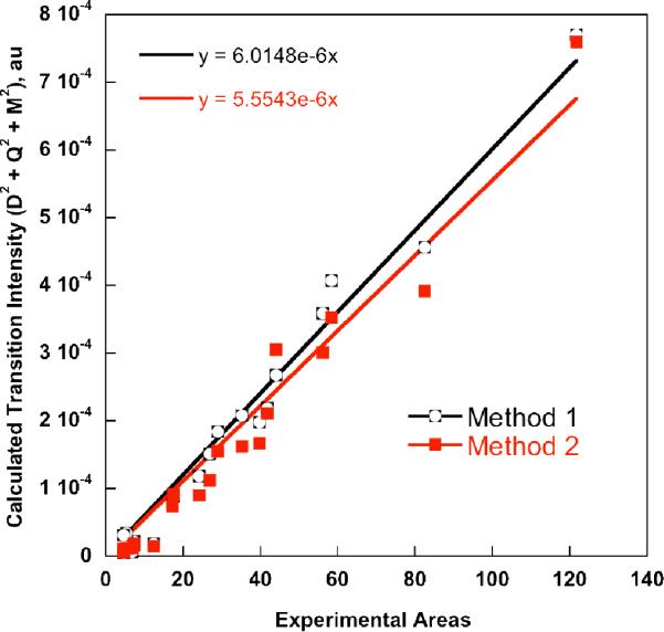
Correlation between the experimental and calculated pre-edge intensities using methods 1 and 2. Experimental areas were obtained using Simpson's rule, as indicated in the methods section and in Table 2.

The observed correlations between experimental and calculated energies and intensities parallel those previously reported when investigating only ferrous and ferric complexes,²⁰ and demonstrate that the predictive ability of these methods does not deteriorate for higher oxidation states or more varied coordination geometries. Figures 3–5 compare the experimental data to the calculated spectra (using Method 2) for the Fe(IV), Fe(V) and Fe(VI) complexes investigated in this study. The comparison clearly demonstrates that the trends in energies, intensities and relative distributions of pre-edge features are well reproduced by the TDDFT calculations. This allows us to analyze the calculations more closely in order to obtain detailed insights into the origin of the observed experimental spectra.

Figure 3.

Comparison of the experimental (A) and calculated (B) Fe K- pre-edge spectra for [Fe(O)(TMC)(MeCN)]²⁺, [Fe(O)(TMCS)]¹⁺ and [Fe(O)(TMC)(O₂CCF₃]¹⁺. A 1.5 eV broadening and a constant shift of 53.9 eV have been applied to the calculated spectra.

Figure 5.

Comparison of the experimental (A) and calculated (B) Fe K- pre-edge spectra for [Fe(N)(PhBP^iPr₃)]²⁺, [Fe(N₃)(Cyc-ac)]²⁺, [Fe(N)(Cyc-ac)]¹⁺, and [Fe(N)(Me₃Cyc-Ac)]²⁺. A 1.5 eV broadening and a constant shift of 53.9 eV have been applied to the calculated spectra.

Figure 3 shows a comparison of the experimental and calculated Fe K- pre-edge data for [Fe(O)(TMC)(MeCN)]²⁺, [Fe(O)(TMC)(O₂CCF₃]¹⁺, and [Fe(O)(TMCS)]¹⁺. The experimental data show the largest intensity for [Fe(O)(TMC)(O₂CCF₃]¹⁺ (39 units of intensity, using Simpson's rule), with a slight decrease on going to [Fe(O)(TMC)(MeCN)]²⁺ (35 units) and a more pronounced effect on going to the thiolate ligated [Fe(O)(TMCS)]¹⁺ (24 units). This 1.1 to 1.0 to 0.7 experimental ratio of areas is reasonably well reproduced by the scalar relativistic calculations, which provide a 1.1 to 1.0 to 0.6 calculated intensity ratio for this series. Note that using method 1, without relativistic corrections, the intensity ratio for the [Fe(O)(TMC)(MeCN)]²⁺ and [Fe(O)(TMC)(O₂CCF₃)]¹⁺ complexes is reversed. This is not necessarily a failure of the theoretical protocol, as the difference in the experimental areas is within the error of the fitting procedure (Table 2). Importantly, the more pronounced changes in the thiolate ligated complex are faithfully reproduced by both computational methods. The pronounced decrease in the thiolate pre-edge intensity derives from the strong trans effect of the axial sulfur, which experimentally elongates the Fe-oxo bond by ~0.05 Å. This trend is reproduced in both the BP86 and B3LYP optimized geometries, which show a ~0.04 Å elongation of the Fe-oxo bond in the thiolate complex relative to the NCCH₃ and O₂CCF_3⁻ ligated TMC complexes. The elongation is accompanied by a ~5% decrease of 4p character in the d-orbitals in the NCCH₃ and O₂CCF_3⁻ ligated TMC complexes and a decreasing of ~3% in the thiolate complex. This decrease in d/p mixing is paralleled by a loss of pre-edge intensity. This result highlights the importance of ligand-metal covalency in modulating pre-edge intensity, as has been previously discussed.^8,9,55,56

Figures 4A and B present the experimental and calculated spectra for [Fe(O)(N4Py)]²⁺, [Fe(O)(TMG₃tren)]²⁺, [Fe(O)(TAML)]²⁻, and [Fe(O)(TAML)]¹⁻. This series allows for the evaluation of both spin- and oxidation-state contributions to the Fe K-pre-edge data. The differences in the [Fe(O)(N4Py)]²⁺ and [Fe(O)(TMG₃tren)]²⁺ spectra are dominated by the changes in spin state. The former complex features a S=1 ground state, while the latter represents the first structurally characterized iron(IV) model complex with a ground state total spin of S=2.³⁵ Already before the structure became available, we had predicted that the change of spin state should have a pronounced effect on the pre-edge of the XAS spectra.⁵⁵ This arises because of the more pronounced multiplet splittings for an S=2 spin state. In both cases, the excitation of a core electron into an empty orbital increases the number of unpaired electrons and leads to multiplet splitting as the number of unpaired electrons exceeds the target multiplicity. In the case of an S=1 ground state, there are three linearly independent spin-functions (Scheme 2), whereas in the case of S=2 there are five linearly independent spin couplings (Scheme 3). In principle, all of these spin couplings correspond to physically realizable states that can be experimentally observed. The original derivation⁵⁵ showed that for a S=1 ground state the energetic separation between the energetically lowest and highest spin coupling is $\frac{14}{5}{K}_{dd}$, where K_dd is an average exchange integral between the metal d-based orbitals. In the case of an S=2 ground state this splitting is $\frac{5}{3}{K}_{dd}$. This much larger splitting arises because for an S=2 ground state each unpaired electron feels a stronger exchange field simply because there are more unpaired electrons than in the case of an S=1 ground state. This results in two clearly observable pre-edge features in the S=2 case, as observed experimentally for both [Fe(O)(TMG₃tren)]²⁺ and the TauD Fe(IV)-oxo intermediate (vide infra). The difference of almost 2K_dd can be translated to the Racah parameter using the estimate: K_dd ≈ B + C ≈ 5B. Since the Racah parameter B is on the order of 1000–1200 cm⁻¹, an increased splitting of about 10B ≈ 10,000–12,000 cm⁻¹ (1.2–1.5 eV) can be expected upon increasing the spin state from S = 1 to S= 2.

Figure 4.

Comparison of the experimental (A) and calculated (B) Fe K- pre-edge spectra for [Fe(O)(N4Py)]²⁺, [Fe(O)(TMG₃tren)]²⁺, [Fe(O)(TAML)]²⁻, and [Fe(O)(TAML)]¹⁻. A 1.5 eV broadening and a constant shift of 53.9 eV have been applied to the calculated spectra.

Scheme 2.

Branching diagrams illustrating the three linearly independent spin couplings that arise from coupling four unpaired electrons in four orbitals to a total spin of S=1 (x-axis: singly occupied orbital; y-axis: total spin).

Scheme 3.

Branching diagrams illustrating the five linearly independent spin couplings that arise from coupling six unpaired electrons in six orbitals to a total spin of S=2 (x-axis: singly occupied orbital; y-axis: total spin).

Unfortunately, the TDDFT calculations are unable to correctly reproduce this multiplet splitting because in the spin-polarized picture the shell-opening excitations only lead to two excited determinants, neither of which corresponds to a pure spin state of the target multiplicity. Thus, the “spin-polarization” observed in open-shell TDDFT calculations should be regarded as a “poor man's approximation” to the multiplet splittings that are observable in the actual spectra. The effect shows up in spin-up and spin-down acceptor orbitals that have different orbital energies and hence, lead to different transition energies for the corresponding spin-up and spin-down transitions. Nevertheless, it is remarkable that the calculated splitting matches the observed spectra surprisingly well (Tables 2 and 3). Taken together, the experimental data and the calculations demonstrate that this is in fact the case, and that XAS data have a much larger contribution from the metal ground state spin than has been generally appreciated.

The effect of the metal oxidation state is perhaps best viewed by comparing [Fe(IV)(O)(TAML)]²⁻ and [Fe(V)(O)(TAML)]¹⁻. The data and calculations clearly show that the effect of oxidation state and the associated structural changes in the iron-oxo bond lengths are reflected in the pre-edge energies and intensities. On going from [Fe(IV)(O)(TAML)]²⁻ to the [Fe(V)(O)(TAML)]¹⁻, the pre-edge increases by 0.8 eV in energy. This trend is reasonably well reproduced by the calculations, which show a 0.6 eV increase in energy. Inspection reveals that this dominantly reflects the increase in the energy of the d_z²-based molecular acceptor orbital, which arises primarily from a stronger and shorter iron-oxo bond (1.64 Å for [Fe(IV)(O)(TAML)]²⁻ vs 1.59 Å for [Fe(V)(O)(TAML)]¹⁻).^10,57

Figures 5A and B present the experimental and calculated spectra for [Fe(N)(PhBP^iPr₃)]²⁺, [Fe(N₃)(Cyc-ac)]²⁺, [Fe(N)(Cyc-ac)]¹⁺, and [Fe(N)(Me₃Cyc-Ac)]²⁺. The Fe K- pre-edge feature of [Fe(N)(PhBP^iPr₃)]²⁺ appears at lowest energy and has by far the most intense pre-edge area of all complexes examined. The relatively low pre-edge energy (7112.4 eV) presumably results from the 4-coordinate, low-spin (s=0) environment, which reduces the ligand field and hence, also decreases the pre-edge transition energy. The high intensity derives from the T_d geometry, which allows for greater 3d–4p mixing to occur. This mixing is further enhanced by the very short 1.52 Å Fe-N (nitrido bond). The combination of both effects leads to an impressive iron pre-edge with more than 94 units of intensity. The trends in the [Fe(III)(N₃)(Cyc-ac)]²⁺, [Fe(V)(N)(Cyc-ac)]¹⁺, and [Fe(VI)(N)(Me₃Cyc-Ac)]²⁺ series are also well reproduced by the calculations. As expected, the azide complex has the lowest intensity, which derives from the relatively long Fe-N(azide) bond (1.83 Å) and the near O_h geometry (the Fe is situated only 0.083 Å above the plane of the macrocycle). Upon oxidation to the Fe(V)-nitrido state, the pre-edge dramatically increases in energy and intensity as a result of the short nitrido bond (1.64 Å) and the coupled displacement of the iron from the plane of the macrocycle (by ~0.12 Å). On going to the Fe(VI)-nitrido, the Fe-N(nitrido) bond becomes even shorter (1.53 Å) resulting in even larger intensity.⁹

It is of interest to note that the pre-edge intensities of all the nitrido complexes are higher than those of the corresponding oxo complexes. This is consistent with the higher covalency of the Fe-nitrido bond and a resultant larger trans effect.⁵⁵

Discussion and extension to protein intermediates

In the current study, we have broadened the calibration of the methodology developed for ferrous and ferric complexes to span Fe(II), Fe(III), Fe(IV), Fe(V) and Fe(VI) complexes. The correlation of calculated energies and intensities to the experimental values remains linear through this wide range of oxidation states. Importantly, the relative distribution of spectral features is well reproduced by these methods. This demonstrates that TDDFT provides a powerful tool for not only reproducing and assigning spectra of known complexes, but also has the potential for predicting spectra. To this end we have extended the TDDFT calibration of model complexes to high-valent species in enzyme intermediates. Specifically the spectra for both the oxo Fe(IV) intermediate in taurine/α-ketoglutarate dioxygenase (TauD) and the Compound II intermediate in P450 were calculated (Figure 6). Fe K-edge XAS spectra of the TauD Fe(IV)-oxo intermediate have been previously reported.⁶ Data are also available for the chloroperoxidase Compound II intermediate, which has served as an analogue for understanding P450.¹ In both cases, the experimental Fe K- pre-edge data have not been analyzed in detail.

Figure 6.

Optimized structures of intermediate in TauD-J (left) and CPO Compound II (right).

Figure 7 presents the experimental data and the corresponding calculated spectrum for the Fe(IV)-oxo intermediate of TauD. The calculated spectrum predicts 29 units of intensity with a maximum at 7113.3 eV. This is in good agreement with the experimental data that show 27 units of intensity and a peak at 7113.1 eV.⁶ The relative energy and the splitting of the peaks are manifestly well reproduced. The lower energy features correspond primarily to a spin-up Fe 1s → 3d_z² transition. To higher energy one finds the corresponding spin-down transitions. This situation approximately describes the significant multiplet splittings described above. Hence in the protein, as in the S=2 model complexes, the higher spin state makes a clear contribution to the overall spectral shape and provides a marker for changes in the electronic structure.

Figure 7.

Comparison of the experimental XAS pre-edge data for the Fe(IV)-oxo intermediate of TauD (A) together with a representative fit to the data and (B) the TDDFT calculated pre-edge of TauD. The gray sticks correspond to the individual transitions that comprise the total spectrum. A 1.5 eV broadening and a constant shift of 53.9 eV have been applied to the calculated spectra.

Figure 8 presents the calculated spectra for Fe(IV)-oxo and Fe(IV)-OH Compound II intermediates of the heme enzyme P450. Detailed studies by Green and coworkers on chloroperoxidase (CPO) have shown that this intermediate is best described as a protonated ferryl species;¹ however, this assignment has been the subject of some controversy.²¹ In order to further investigate this question, we have compared the calculated Fe(IV)-oxo and Fe(IV)-hydroxo species to the previously published experimental data for chloroperoxidase compound II, which showed a pre-edge with ~15 units of intensity centered at 7113.3 eV. For the Fe(IV)-oxo species, the calculation predicts 29 units of intensity centered at ~7113.3 eV. For a Fe(IV)-hydroxo species, the calculation predicts 10 units of pre-edge intensity, centered at ~7113.0 eV. The decrease in intensity and slight decrease in transition energy are readily attributed to the lengthening of the axial Fe-O bond upon protonation. The lengthening results in a decrease of the 3d_z²-4p_z mixing, thus decreasing both the ligand field and the pre-edge intensity. Obviously, the calculated spectrum of the protonated species is in considerably better agreement with the experimental spectrum than that of the oxo species, thus lending further credence to the analysis by Green and co-workers.

Figure 8.

Comparison of the calculated XAS pre-edge data for an Fe(IV)-oxo and Fe(IV)-OH intermediates of compound II. A 1.5 eV broadening and a constant shift of 53.9 eV have been applied to the calculated spectra.

It is also of interest to note that the initial assignment of a protonated ferryl species in CPO was based largely on EXAFS data, which are considerably more challenging to obtain than edge data for dilute radiation-sensitive metalloprotein samples. The current study highlights that considerable information about the local iron environment can be obtained from the pre-edge data alone, provided that the measurements are carefully combined with quantum chemical calculations.

Conclusions

In summary, this work demonstrates that the TDDFT methodology previously developed for Fe(II) and Fe(III) complexes is readily extended to Fe(IV), Fe(V) and Fe(VI) complexes. Generally very good agreement is obtained between the calculated energies and intensities, as well as the relative distributions of features. The splitting to the pre-edge features in high-spin Fe(IV) complexes further highlights the sensitivity of this method to spin state. Finally, we have shown that TDDFT methods can be used to obtain insights into the local geometric and electronic structures of high-valent iron protein intermediates. Thus these methods serve to complement structural data, which can be obtained for EXAFS. These methods have a potential advantage in cases where obtaining EXAFS data may be prohibitive. In any case, we hope that the present investigations demonstrate that the combination of XAS spectroscopy and quantum chemistry opens many exciting possibilities for the future investigation of model complexes, metalloenzymes and related systems.

References

- (1).Green MT, Dawson JH, Gray HB. Science. 2004;304:1653. doi: 10.1126/science.1096897. [DOI] [PubMed] [Google Scholar]
- (2).Denisov IG, Makris TM, Sligar SG, Schlichting I. Chem. Rev. 2005;105:2253. doi: 10.1021/cr0307143. [DOI] [PubMed] [Google Scholar]
- (3).Sono M, Roach MP, Coulter ED, Dawson J. H. Chem. Rev. 1996;96:2841. doi: 10.1021/cr9500500. [DOI] [PubMed] [Google Scholar]
- (4).Solomon EI, Brunold TC, Davis MI, Kemsley JN, Lee SK, Lehnert N, Neese F, Skulan AJ, Yang YS, Zhou J. Chem. Rev. 2000;100:235. doi: 10.1021/cr9900275. [DOI] [PubMed] [Google Scholar]
- (5).Krebs C, Fujimori DG, Walsh CT, Bollinger JM., Jr Acc. Chem. Res. 2007;40:484. doi: 10.1021/ar700066p. [DOI] [PMC free article] [PubMed] [Google Scholar]
- (6).Riggs-Gelasco PJ, Price JC, Guyer RB, Brehm JH, Barr EW, Bollinger JM, Krebs C. J. Am. Chem. Soc. 2004;126:8108. doi: 10.1021/ja048255q. [DOI] [PubMed] [Google Scholar]
- (7).Rittle J, Green MT. Science. 2010;330:933. doi: 10.1126/science.1193478. [DOI] [PubMed] [Google Scholar]
- (8).Aliaga-Alcalde N, Mienert B, Bill E, Wieghardt K, George SD, Neese F. Angew. Chem. Int. Ed. 2005;44:2908. doi: 10.1002/anie.200462368. [DOI] [PubMed] [Google Scholar]
- (9).Berry JF, Bill E, Bothe E, George SD, Mienert B, Neese F, Wieghardt K. Science. 2006;312:1937. doi: 10.1126/science.1128506. [DOI] [PubMed] [Google Scholar]
- (10).de Oliveira FT, Chanda A, Banerjee D, Shan X, Mondal S, Que L, Jr., Bominaar EL, Münck E, Collins TJ. Science. 2007;315:835. doi: 10.1126/science.1133417. [DOI] [PubMed] [Google Scholar]
- (11).England J, Martinho M, Farquhar ER, Frisch JR, Bominaar EL, Munck E, Que L., Jr Angew. Chem. Int. Ed. 2009;48:3622. doi: 10.1002/anie.200900863. [DOI] [PMC free article] [PubMed] [Google Scholar]
- (12).Grapperhaus CA, Mienert B, Bill E, Weyhermuller T, Wieghardt K. Inorg. Chem. 2000;39:5306. doi: 10.1021/ic0005238. [DOI] [PubMed] [Google Scholar]
- (13).Jackson TA, Rohde J-U, Seo MS, Sastri CV, DeHont R, Stubna A, Ohta T, Kitagawa T, Mu∞nck E, Nam W, Que L., Jr J. Am. Chem. Soc. 2008;130:12394. doi: 10.1021/ja8022576. [DOI] [PMC free article] [PubMed] [Google Scholar]
- (14).Bell CB, Wong SD, Xiao YM, Klinker EJ, Tenderholt AL, Smith MC, Rohde JU, Que L, Jr., Cramer SP, Solomon EI. Angew. Chem. Int. Ed. 2008;47:9071. doi: 10.1002/anie.200803740. [DOI] [PMC free article] [PubMed] [Google Scholar]
- (15).Decker A, Rohde JU, Klinker EJ, Wong SD, Que L, Jr., Solomon EI. J. Am. Chem. Soc. 2007;129:15983. doi: 10.1021/ja074900s. [DOI] [PMC free article] [PubMed] [Google Scholar]
- (16).Rohde J-U, Torelli S, Shan X, Lim MH, Klinker EJ, Kaizer J, Chen K, Nam W, Que L., Jr J. Am. Chem. Soc. 2004;126:16750. doi: 10.1021/ja047667w. [DOI] [PubMed] [Google Scholar]
- (17).Westre TE, Kennepohl P, DeWitt JG, Hedman B, Hodgson KO, Solomon EI. J. Am. Chem. Soc. 1997;119:6297. [Google Scholar]
- (18).Jin N, Ibrahim M, Spiro TG, Groves JT. J. Am. Chem. Soc. 2007;129:12416. doi: 10.1021/ja0761737. [DOI] [PMC free article] [PubMed] [Google Scholar]
- (19).Song WJ, Seo MS, DeBeer George SO,T, Song R, Kang MJ, Tosha T, Kitagawa T, Solomon EI, Nam W. J. Am. Chem. Soc. 2007;129:1268. doi: 10.1021/ja066460v. [DOI] [PMC free article] [PubMed] [Google Scholar]
- (20).DeBeer George S, Petrenko T, Neese F. J. Phys. Chem. A. 2008;112:12936. doi: 10.1021/jp803174m. [DOI] [PubMed] [Google Scholar]
- (21).Newcomb M, Halgrimson JA, Horner JH, Wasinger EC, Chen LX, Sligar SG. Proc. Natl. Acad. Sci. U.S.A. 2008;105:8179. doi: 10.1073/pnas.0708299105. [DOI] [PMC free article] [PubMed] [Google Scholar]
- (22).Bukowski MR, Koehntop KD, Stubna A, Bominaar EL, Halfen JA, Münck E, Nam W, Que L., Jr Science. 2005;310:1000. doi: 10.1126/science.1119092. [DOI] [PubMed] [Google Scholar]
- (23).Arutyunyan LD, Ponomarev VI, Atovmyan LO, Lavrent'eva EA, Lavrent'ev IP, Khidekel ML. Koord. Khim. (Russ. Coord. Chem. 1979;5:943. [Google Scholar]
- (24).Betley TA, Peters JC. J. Am. Chem. Soc. 2004;126:6252. doi: 10.1021/ja048713v. [DOI] [PubMed] [Google Scholar]
- (25).Brown SJ, Olmstead MM, Mascharak PK. Inorg. Chem. 1990;29:3229. [Google Scholar]
- (26).Gerloch M, Mabbs FE. J. Chem. Soc. A. 1967:1598. [Google Scholar]
- (27).Klinker EJ, Kaizer J, Brennessel WW, Woodrum NL, Cramer CJ, Que L., Jr Angew. Chem. Int. Ed. 2004;44:3690. doi: 10.1002/anie.200500485. [DOI] [PubMed] [Google Scholar]
- (28).Kuchar J, Cernak J, Massa W. Acta Crystallogr. C. 2004;C60:m418. doi: 10.1107/S0108270104014581. [DOI] [PubMed] [Google Scholar]
- (29).Lauher JW, Ibers JA. Inorg. Chem. 1975;14:348. [Google Scholar]
- (30).Rohde J-U, In J-H, Lim MH, Brennessel WW, Bukowski MR, Stubna A, Münck E, Nam W, Que L., Jr Science. 2003;299:1037. doi: 10.1126/science.299.5609.1037. L. [DOI] [PubMed] [Google Scholar]
- (31).George GN. EXAFSPAK, SSRL, SLAC. Stanford University; Stanford, CA: [Google Scholar]
- (32).Tenderholt A. PySpline. Stanford Synchrotron Radiation Laboratory, Stanford Linear Accelerator Center, Stanford University; Stanford, CA: [Google Scholar]
- (33).Kistenmacher TJ, Stucky GD. Inorg. Chem. 1867;7:2150. [Google Scholar]
- (34).Overgaard J, Svendsen H, Chevalier MA, Iversen BB. Acta Crystallogr. E. 2005;E61 [Google Scholar]
- (35).England J, Guo Y, Farquhar ER, Young VG, Jr., Munck E, Que L., Jr J. Am. Chem. Soc. 2010;132:8635. doi: 10.1021/ja100366c. [DOI] [PMC free article] [PubMed] [Google Scholar]
- (36).Rohde J-U, Betley TA, Jackson TA, Saouma CT, Peters JC, Que L., Jr Inorg. Chem. 2007;46:5720. doi: 10.1021/ic700818q. [DOI] [PMC free article] [PubMed] [Google Scholar]
- (37).Neese F, Becker U, Ganyushin D, Hansen A, Liakos DG, Kollmar C, Kossmann S, Petrenko T, Reimann C, Riplinger C, Sivalingam K, Valeev E, Wezisla B, Wennmohs F.
- (38).Becke AD. Phys. Rev. A. 1988;38:3098. doi: 10.1103/physreva.38.3098. 38. [DOI] [PubMed] [Google Scholar]
- (39).Perdew JP. Phys. Rev. B. 1986;33:8822. doi: 10.1103/physrevb.33.8822. [DOI] [PubMed] [Google Scholar]
- (40).Schafer A, Huber C, Ahlrichs R. J. Chem. Phys. 1994;100:5829. [Google Scholar]
- (41).Neese F. Inorg. Chim. Acta. 2002;337C:181. [Google Scholar]
- (42).van Lenthe E, Baerends EJ, Snijders JG. J. Chem. Phys. 1993;99:4597. [Google Scholar]
- (43).Van Wüllen CJ. J. Chem. Phys. 1998;109:382. [Google Scholar]
- (44).Pantazis DA, Chen X-Y, Landis CR, Neese F. J. Chem. Theory Comput. 2008;4:908. doi: 10.1021/ct800047t. [DOI] [PubMed] [Google Scholar]
- (45).Pantazis DA, Neese F. J. Chem. Theory Comput. 2009;5:2229. doi: 10.1021/ct900090f. [DOI] [PubMed] [Google Scholar]
- (46).Pantazis DA, Neese F. J. Chem. Theory Comput. 2011;7 doi: 10.1021/ct900090f. [DOI] [PubMed] [Google Scholar]
- (47).DeBeer George S, Neese F. Inorg. Chem. 2010;49:1849. doi: 10.1021/ic902202s. [DOI] [PubMed] [Google Scholar]
- (48).Devlin FJ, Finley JW, Stephens PJ, Frisch MJ. J. Phys. Chem. 1995;99:16883. [Google Scholar]
- (49).Klamt A, Schüürmann G. J. Chem. Soc. Perkin Trans. 1993;2:799. [Google Scholar]
- (50).Elkins JM, Ryle MJ, Clifton IJ, Dunning Hotopp JC, Lloyd JS, Burzlaff NI, Baldwin JE, Hausinger RP, Roach PL. Biochemistry. 2002;41:5185. doi: 10.1021/bi016014e. [DOI] [PubMed] [Google Scholar]
- (51).Perdew JP, Burke K, Ernzerhof M. Phys. Rev. Lett. 1996;77:3865. doi: 10.1103/PhysRevLett.77.3865. [DOI] [PubMed] [Google Scholar]
- (52).Grimme S. J. Comput. Chem. 2006;27:1787. doi: 10.1002/jcc.20495. [DOI] [PubMed] [Google Scholar]
- (53).Siegbahn PEM, Blomberg MRA, Chen SL. J. Chem. Theory Comput. 2010;6:2040. doi: 10.1021/ct100213e. [DOI] [PubMed] [Google Scholar]
- (54).Siegbahn PEM, Blomberg MRA. Chem. Rev. 2000;100:421. doi: 10.1021/cr980390w. [DOI] [PubMed] [Google Scholar]
- (55).Berry JF, DeBeer George S, Neese F. Phys. Chem. Chem. Phys. 2008;10:4361. doi: 10.1039/b801803k. [DOI] [PubMed] [Google Scholar]
- (56).DeBeer George S, Brant P, Solomon EI. J. Am. Chem. Soc. 2005;127:667. doi: 10.1021/ja044827v. [DOI] [PubMed] [Google Scholar]
- (57).Chanda A, Shan X, Chakrabarti M, Ellis WC, Popescu DL, de Oliveira FT, Wang D, Que L, Jr., Collins TJ, Münck E, Bominaar EL. Inorg. Chem. 2008;47:3669. doi: 10.1021/ic7022902. [DOI] [PMC free article] [PubMed] [Google Scholar]
Associated Data
This section collects any data citations, data availability statements, or supplementary materials included in this article.