Quantifying the longitudinal value of healthcare record collections for pharmacoepidemiology

Abstract

We introduce an information score for longitudinal healthcare record data, specifically in the monitoring of chronic conditions. The score is designed to capture the value of different observation patterns in terms of shaping and testing clinical epidemiological hypotheses. The score is first developed for the simple case where equally spaced observations are most informative, then extended to a more context-specific version where the optimal density of observations can be elicited. It can be interpreted as a measure of the average quantity of information provided by each observation in an individual’s time course, where information is lost whenever the observation density deviates from a defined optimal density.

We illustrate the score on routine healthcare records from the population of Salford, UK – focusing on repeat testing of liver function in people with common long-term conditions. We demonstrate validity of the score in terms of concordance between score levels and clinically meaningful patterns of repeat testing.

Introduction

Most of the safety, effectiveness, cost effectiveness and acceptability of drug treatments in the real world is unknown¹. Randomized controlled trials (RCTs) provide high quality evidence but with limited generalizability, for example to those taking other medications because such patients are usually excluded from trials². With the increasing quality, quantity, structure and availability of electronic health record data for research there is an opportunity to expand pharmacoepidemiology to fill this gap in evidence. Such research, however, is fraught with analytical difficulties due to the naturalistic nature of the data. Clinical practice lacks the careful experimental design of RCTs, introducing problems such as confounding by indication, unmeasured confounding, time-varying exposure patterns, time-varying data capture and missing data.

Despite the informatic and statistical difficulties in using healthcare records for research there is potential scientific value in exploiting the differences between healthcare settings in this way. Observational clinical research might be improved by exploiting heterogeneity – combining similar studies while incorporating (meta)data on the differences between the studies³. In order to achieve both useful heterogeneity and large sample size investigators may have to deal with multiple databases of coded clinical records⁴. Pharmacoepidemiology studies often tackle complex patterns of drug treatment and outcomes over time. Drug safety studies in particular are putting more emphasis on intermediate outcomes, such as trend in liver enzymes, rather than relying on adverse event reports, e.g. around acute liver conditions. So there is a need for tools to help investigators to assess the longitudinal value of records from different sources of data that may be incorporated into a pharmacoepidemiology study.

We consider the situation in which patients are subject to repeated measurements over time. A simple assessment of the longitudinal value of an individual patient can be obtained by combining the length of time for which the patient is observed, with the number of observations made over that time. Dividing the latter by the former gives an ‘observation rate’ – the number of observations made per unit time.

However, this does not take into account the regularity with which observations are made. Consider a patient with a cluster of observations at the beginning and end of a long observation period – this patient’s record provides relatively little longitudinal information when compared with a patient who has the same number of observations spaced evenly over the same period: non-linearity of response can only be measured for the latter patient. Some observers may fail to notice the distinction between these two situations, leading them to incorrectly value the two situations equally.

In this paper, we focus on the case in which it is optimal to have observations spaced evenly over time. This is the typical case where a physiological measure is used to monitor the progression of a chronic disease, for example kidney function in diabetics estimated from creatinine, age and sex (± ethnicity). Many patients with chronic diseases are in a program of care that includes regular measurement of common pathophysiological indicators such as blood pressure, urea and electrolytes, full blood count and liver enzymes. During acute exacerbations of chronic conditions more testing is often done – so the density of records over time may correlate with the course of the disease determined by factors other than those under study. It is important to have expert, local clinical interpretation of such patterns. We recognize the need for tools to help local clinicians and researchers to explore longitudinal patterns in clinical record collections together.

In this paper we introduce a new tool, an information score, to help researchers and clinicians to measure the potential longitudinal value of a given observation repeated across a series of healthcare records.

Methods

We develop an information score that accounts for the typical irregularity of healthcare measurements. For simplicity of exposition, we suppose in the first instance that the optimal situation is to have equally spaced observations – the assumption on which much chronic disease management is based. Then we extend this measure to other patterns of observation.

For each patient, a number I, between 0 and 1, denotes the average amount of information that each observation provides. In order to calculate the information score, suppose, for a patient observed n times, the ordered observation times are x₍₁₎, …, x_(n). For i = 1, …, n – 1, let $g_i=\frac{x_{(i+1)}-x_{(i)}}{x_{(n)}-x_{(1)}}$, the relative time gaps between observations. Then, the formula for calculating I is given by:-

$$I=\frac{2}{n}+\frac{n-2}{n}\left[1-\sqrt{(n-1)\text{Var}\{g_i;i=1,\dots ,n–1\}}\right].$$

The simple optimal situation, I = 1, corresponds to equally spaced observations. The worst case, I = 2/n, corresponds to the observations being made at two distinct times only, namely the start and end of the observation period. We define n_e = I × n as the effective number of observations available for each patient. This motivates the range of the formula, since n_e = 2 for the case where observations are made at two distinct times only, and n_e = n for the optimal case of equally spaced observations. We also define $d_e=\frac{n_e}{x_{(n)}-x_{(1)}}$, the effective density: the effective number of observations made per unit time for each patient.

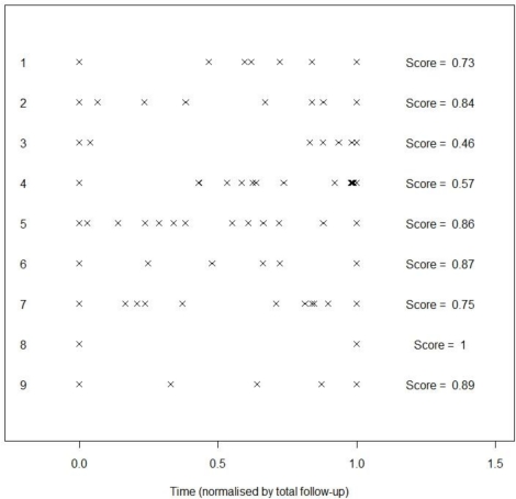
The main driver of the quality of information I is the variability of the time gaps between observations. For an example, see Figure 1. In this Figure, observations have been scaled so that the first and last observations, x₍₁₎ and x_(n), are in the same place for each patient. Individual 8 has only two observations, so I = 1 since the observations are equally spaced. Individual 3 has I = 0.46; this low number arises since the observations are in two clusters, near the beginning and near the end of the observation period.

Figure 1.

Examples of information scores for various patterns of measurement of a long term condition.

In practice, the information score carries little meaning on its own, and is best used in combination, with the number of observations, through n_e, or the density, through d_e.

A number of extensions to the scoring method can be considered:

For the first extension, it may be the case that data is sought for a particular calendar time interval [a, b] – representing say a meaningful interval before and after the introduction of a new prescribing guideline. Then, we would like to assign less value to individuals whose observations give poor coverage of the interval of interest. Hence a revised information score can be calculated in this scenario:-

$$I^{*}=I\times \frac{\text{min}\left\{b,x_{(n)}\right\}-\text{max}\{a,x_{(1)}\}}{b-a}.$$

Consider the case where we have 10 daily observations and 10 monthly observations. The original definition, I, of the information score would assign both of these scenarios the same score. However, we might demand at least 10 months of observation – either to cover a specific period of interest or to give a clinically meaningful length of follow-up. The revised measure I^* would then penalize the daily information heavily, but not the monthly information.

For the second extension, we consider the case where a higher density of observations is sought at specific points in time, rather than regularly repeated observations. A natural way to revise the information score to take account of the specific time point is by re-calculating the gaps g_i on a re-scaled time axis. Let f (t) be a function that describes our interest in the time point t. The function f (t) should be normalized so that ∫ f (t)dt =1. Then, the revised calculation for each g_i is given by:-

$$g_i={\int }_{x_{(i)}}^{x_{(i+1)}}f(t)dt.$$

Note that the original derivation of the gaps is a special case of this formulation, taking a uniform density:-

$$f(t)=\{\begin{array}{cc}{\left(x_{(n)}-x_{(1)}\right)}^{-1}& x_{(1)}\le t\le x_{(n)}\\ 0& \text{otherwise.}\end{array}$$

Such a strategy can be useful in a range of scenarios. First, in a clinical trial, observations may be more valuable once the drug being tested has reached its maximum concentration. Second, if a treatment transition is thought to influence the quantity of interest, setting t = 0 at the time of the treatment transition and constructing a function f (t) with a peak at t = 0 would assign a relevant information score for identifying patients with sufficient power to test such a hypothesis. Deriving a suitable function f (t) is a challenging issue. For a clinical trial, one could define it in terms of the drug concentration curve; in a more general setting, one could use expert elicitation to establish the time periods of interest.

For the third extension, we consider the case where there is a threshold to reach before an observation becomes clinically apparent, and where a slowly developing background risk may suddenly accelerate into frank disease – for example in cancer screening. In high risk groups in particular, observations must be sufficiently frequent to detect a new lesion while it is treatable. Suppose that the time interval in which a ‘pre-cancer’ develops into a ‘malignancy’ is given by δ. Then one way in which the information score can be assigned is to consider the probability that the lesion is detected in time (assuming it is uniformly likely to develop over the observation interval) is:-

$$I\prime =\frac{{\sum }_{i=1}^{n-1}\text{max}\{x_{(i+1)}–x_{(i)}–\delta ,0\}}{x_{(n)}–x_{(1)}}.$$

Example

Salford is a city in Greater Manchester, UK, with a population of 218,000. The Salford Integrated Record (SIR) combines the healthcare records from primary and secondary care for more than 97% of the population. The data in the SIR is derived from general practice consultations, referrals, clinic attendances, laboratory tests and hospital episodes, from around the year 2000 to the present.

To illustrate the methodology of the information score, we take a subset of the SIR, corresponding to patients with at least one of the following long term conditions: type I and type II diabetes; coronary heart disease; cerebrovascular disease; chronic kidney disease; and chronic liver disease, and at least one liver function test for alanine transaminase (ALT). This provides us with a sample size of 30,366 patients. The relevance of the information score in this context is that patients with these long term conditions have routine ALT monitoring, but the spacing of results over time is highly uneven. This irregularity is not due to inconsistent data capture because all of the test results from the main laboratory were available and patient identifiers were reliable. The irregularity reflects variations in clinical practice, disease and patient concordance with chronic disease management. So the time course of real world biochemical records is often irregular and of varying density. There are no reliable variables with which to instrument the irregularity and differences in the test density between patients. For our study, the numbers of ALT tests taken by patients in the sample range from 1 to 289, with a median of 9, and an interquartile range of 9.

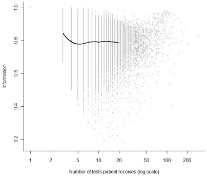
The distribution of the information score I, plotted against the number of tests for each patient, n, is given in Figure 2. The grey dots correspond to individual patients; the thick black line shows the average level of information at differing numbers of individual tests. This is plotted only between 3 and 20: I = 1 by construction for 1 or 2 observations, and there are relatively few patients with more than 20 tests, making estimation unreliable beyond this. The average value of I tends to be fairly stable at a level of around I = 0.8, hence appears to have little dependence on the number of observations in this particular example. For further intuition we pick out an individual with a low I score from the data: there is an individual with 12 tests and a score of I = 0.190, corresponding to an effective number of tests n_e = 2.28. The individual has tests over 860 days, with the times of the tests given by the sequence: 0, 838, 843, 843, 843, 845, 846, 847, 852, 856, 857, 860. Eleven of the twelve tests take place in the final 2.6 % of the follow-up time, with three of these tests occurring on the same day (day 843).

Figure 2.

Plot of information score against the number of ALT tests a patient receives. The grey dots are individual patients. The black line is an estimate of the average level of information by number of tests.

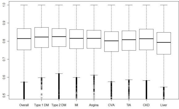
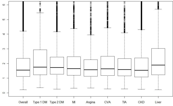
Boxplots for the information density for patients suffering from each chronic disease are given in Figure 3. Note that due to comorbidity, many patients will be contributing to multiple box plots. Differences in the information score, i.e. testing regularity, are small between diseases. Liver disease patients have a smaller median and lower quartile than the other diseases. This should be interpreted in conjunction with the effective density, d_e, of the tests; boxplots of this quantity for the various diseases are given in Figure 4. We see here that liver disease patients have the highest median effective density, with type 1 diabetics also having a high median and upper quartile. Hence, the low median information score for liver disease patients is more than offset by the large number of tests carried out on these patients.

Figure 3.

Boxplots of information score for patients overall, then separately for different sub-groups with: types 1 & 2 diabetes mellitus (DM); myocardial infarction (MI); angina; stroke/cerebrovascular attack (CVA); mini-stroke/transient ischaemic attack (TIA); chronic kidney disease (CKD); and liver disease..

Figure 4.

Boxplots of effective test density for patients overall, then separately for different sub-groups with: types 1 & 2 diabetes mellitus (DM); myocardial infarction (MI); angina; stroke/cerebrovascular attack (CVA); mini-stroke/transient ischaemic attack (TIA); chronic kidney disease (CKD); and liver disease.

We can use the information score to identify bias that may be caused by sicker patients being tested more frequently and potentially over a longer period of time. In order to do this, we fit the regression, for each individual,

$$\text{log}(\text{Mean}\hspace{0.17em}\text{ALT}\hspace{0.17em}\text{Level})={\beta }_0+{\beta }_1\text{log}(x_{(n)}-x_{(1)}+1/365)+{\beta }_{2}I+{\beta }_3\text{log}n+\varepsilon .$$

The resulting coefficients, with 95% confidence intervals, are given in Table 1.

Table 1.

Regression coefficients and confidence intervals.

	Point estimate	95% confidence interval
β0	3.874	(3.814,3.934)
β1	−0.022	(−0.027,−0.017)
β2	−0.566	(−0.621,−0.511)
β3	0.031	(0.022,0.040)

We see that even after correcting for the number of tests and the length of follow-up, the information score remains a highly significant predictor of log(Mean ALT level). Patients with a more regular test pattern are expected to have lower ALT levels. A possible explanation for this is that patients with irregular testing patterns have often had a number of tests in rapid succession, which is typically because the patient is in intensive care. Combined inference on β₁ and β₃ suggests that, unsurprisingly, patients with a higher density of tests typically have higher ALT levels. Fitting a marginal model with follow-up time, log(x_(n) – x₍₁₎ + 1/365), as the only predictor gives a coefficient estimate of 0.004 (95% confidence interval [0.001,0.008]), hence this is marginally a weak predictor of mean ALT levels.

There is hence potential for the information score to be used as part of a methodology that adjusts for the ascertainment bias in routine clinical data.

Discussion

We have introduced a scoring method that quantifies the information available for each individual in a longitudinal study, with respect to the spacing of the observations. In a simple version we assume that information is maximized when observations are equally spaced, but we also demonstrate how the methodology can be extended to cases where it is desirable for the density of observations to vary over the time window.

Ascertaining the information available in a longitudinal study is a complex issue, and the methods introduced here are an exploratory tool and not a universal measure. Output from the information score should be assessed for face validity in the clinical context. The score, plus the effective number of observations and effective density, are a low-dimensional summary of complex longitudinal patterns, and not a substitute for an understanding of why these patterns arise in practice. The use of these statistics by someone with relevant clinical knowledge may offer an improvement over the current position of separate statistical and clinical evaluations.

Tools for evaluating ‘real world’ healthcare datasets, with a view to including them in a particular study or not, are needed. This is especially true where researchers may be remote from the collection of the data – for example where the pharmaceutical industry collaborates with multiple centers in pharmacoepidemiology. Many research questions have a longitudinal aspect to them, since they are concerned with the natural histories of diseases and the outcomes of clinical interventions. Before investing the time and resource to perform such an analysis, it is useful to assess the longitudinal strength of the baseline dataset. The development of the information energy score described here represents an important step towards a deeper understanding of the optimal ways in which to establish whether a real world data set is ’fit for purpose’.

We have also illustrated briefly the importance of considering how the longitudinal patterns in the data may be correlated with the responses recorded at the observations. For example, an elevated liver function test may lead to the patient being observed at more regular intervals following this. The scoring methods discussed in this paper could represent a first step in correcting a longitudinal analysis for confounding of test density and elevated or otherwise unusual response.

An important topic for future research is a more precise definition and derivation of the function f (t) that encapsulates the density of information required across the timeframe of interest. More broadly, alternative methods of calculating information in longitudinal studies should be investigated, which may be more appropriate in specific situations. In particular, the context of the data under consideration should always be taken into account.

A limitation of the information score is that it does not account for variable quality of the measurement process, or the relevance of the quantity being measured to the disease of interest. These issues may require a more complete model of the clinical context, which is beyond the scope of simple summarization and this paper.

In conclusion, we have demonstrated new statistical summaries of coded healthcare records to aid the design of naturalistic longitudinal studies. Further research could extend the methods to illuminate more complex patterns specific to research questions. The development of tools such as this is essential for building globally relevant real world evidence, particularly in understanding the outcomes of drug treatment in routine clinical practice.

References

- 1.Fortin M, Dionne J, Pinho G, Gignac J, Almirall J, Lapointe L. Randomized controlled trials: do they have external validity for patients with multiple morbidities. Ann. Fam. Med. 2006;4:104–108. doi: 10.1370/afm.516. [DOI] [PMC free article] [PubMed] [Google Scholar]
- 2.Valderas JM, Starfield B, Sibbald B, Salisbury C, Roland M. Defining comorbidity: implications for understanding health and health services. Ann. Fam. Med. 2009;7(4):357–363. doi: 10.1370/afm.983. [DOI] [PMC free article] [PubMed] [Google Scholar]
- 3.Thompson S, Kaptoge S, White I, et al. Statistical methods for the time-to-event analysis of individual participant data from multiple epidemiological studies. Int. J. Epidemiol. 2010;39:1345–1359. doi: 10.1093/ije/dyq063. [DOI] [PMC free article] [PubMed] [Google Scholar]
- 4.Observational Medical Outcomes Partnership . Points to consider in developing a common semantic data model and terminology dictionary for observational analyses. Rockville, MD: Foundation for the National Institutes of Health; 2009. Accessed at http://omop.fnih.org/sites/default/files/OMOP%20Points%20to%20Consider%20on%20Common%20Data%20Model%203mar2009_Post.pdf on 16 March 2011. [Google Scholar]