Mechanics of peristaltic locomotion and role of anchoring

Abstract

Limbless crawling is a fundamental form of biological locomotion adopted by a wide variety of species, including the amoeba, earthworm and snake. An interesting question from a biomechanics perspective is how limbless crawlers control their flexible bodies in order to realize directional migration. In this paper, we discuss the simple but instructive problem of peristalsis-like locomotion driven by elongation–contraction waves that propagate along the body axis, a process frequently observed in slender species such as the earthworm. We show that the basic equation describing this type of locomotion is a linear, one-dimensional diffusion equation with a time–space-dependent diffusion coefficient and a source term, both of which express the biological action that drives the locomotion. A perturbation analysis of the equation reveals that adequate control of friction with the substrate on which locomotion occurs is indispensable in order to translate the internal motion (propagation of the elongation–contraction wave) into directional migration. Both the locomotion speed and its direction (relative to the wave propagation) can be changed by the control of friction. The biological relevance of this mechanism is discussed.

1. Introduction

Crawling without legs is one of the most fundamental types of biological locomotion and can be observed in a wide variety of species, including the amoeba, earthworm, snail and leech, as well as in mobile cells  [1–6]. The body of a limbless crawler is in contact with the substrate on which it moves over a long distance and continuously interacts with it. This type of locomotion looks qualitatively different from the bipedal or quadrupedal walking of larger animals; an obvious question to ask is how crawlers control their flexible bodies, which have a continuum of degrees of freedom. This question is also related to a current topic in biologically inspired robotics [7], which aspires to create autonomous robots by mimicking animal motions. When crawlers are migrating, forwards–backwards symmetry (in terms of the motion and/or the shape of the body) must be broken in order to select a particular direction of movement. For instance, amoebas extend pseudopods in the direction of movement. For earthworm and leech, elongation–contraction waves that resemble peristaltic motion propagate in a fixed direction along the body axis.

In this paper, we focus on the peristalsis-like locomotion typically observed in earth worm. We consider that the category of the peristalsis-like locomotion includes the locomotion of snail and of some kind of snakes that can move without undulation of the body (e.g. boas and vipers [3]), although it might be inconsistent with the traditional classification [8,9]. The body structure and size of the above animals are very different from each other: for snail and the above-mentioned snakes, the propagation of elongation–contraction wave occurs only around the ventral surface contacting with the substrate. However, we can expect that a common mechanical principle exists in their locomotion, because the internal motion just above the contact interface should be relevant for the locomotion. Hereafter, we inclusively refer the locomotion of the above slender animals as peristaltic locomotion. Also, the locomotion of some kinds of multi-legged animals, such as caterpillar and myriapod, has a similarity with peristaltic locomotion (details will be discussed in §6.1).

It has been well recognized that in order to realize peristaltic locomotion, a peristaltic crawler should form anchors (at which the body grips the substrate to increase sliding resistance locally) on some parts of the contact area. For example, the contracted (thickened) body segments of the earthworm project bristles from inside in order to increase the friction coefficient [2,4]. For the above-mentioned snakes, slight corrugation of the ventral surface occurs coordinating the peristaltic wave; the parts pressed to the substrate play the role of anchors. A cleverly designed example is the snail locomotion [10–12], which depends on the shear thinning behaviour of the mucus that is secreted on the contact interface. This behaviour reduces the frictional resistance of the parts of the contact interface where a larger shear rate is generated by the peristaltic wave, while the low shear rate parts, where the mucus exhibits relatively high frictional resistance, work as anchors. In the above-mentioned multi-legged animals, the anchor effect is caused by touching and gripping the substrate with legs.

Interestingly, the direction in which the peristaltic (elongation–contraction) wave propagates depends on the species. For example, when the terrestrial snail (Helix), sea snail (Pomatias) and ear shell (abalone Haliotis) move forward, the peristaltic wave travels in the tail-to-head direction, whereas it travels in the head-to-tail direction when the earthworm, eelworm (Criconemoides), leech [1,2] and the above-mentioned snake [3] advance. Pioneering biologists [3,4,9] have diagrammatically analysed the kinematics of peristaltic locomotion, and proposed that the locomotion direction is determined by the phase of peristaltic wave at which the anchors are formed. That is, when the anchor is formed in the contracted parts of the body, the locomotion occurs into the direction opposite to the peristaltic wave propagation. This prediction is consistent with the general tendency of actual peristaltic crawlers. However, as the earlier kinematic analysis relies on diagrammatical and verbal considerations, there remain several ambiguities: for example, the arguments are fairly complicated except a specially simple case of rectangular peristaltic wave; mechanical foundation is lacking.

This paper aims at providing a clear mathematical expression for the relationship between locomotion direction and anchoring phase. For this aim, we propose a simple mechanical model for peristaltic locomotion. The body of a peristaltic crawler is regarded as a one-dimensional string located on a substrate exerting a viscous friction force on each part of the system. The sinusoidal peristaltic wave is generated by an active internal tension that mimics muscular action causing peristaltic movement. The anchoring effect is represented by a localized increase of the viscous friction coefficient at the points where the phase of the peristaltic wave has a particular value. With some simplifications (such as neglecting inertial effects), the equation of motion can be given by a linear one-dimensional diffusion equation with a source term. The diffusion coefficient is inversely proportional to the viscous friction coefficient, and the source term represents the physiological action that causes the elongation–contraction wave. By a perturbation treatment on the anchor effect, we obtain a mathematical expression that relates the locomotion speed (including the direction) with the anchoring phase and with other physical parameters concerning the peristaltic movement (wavelength and amplitude of peristaltic wave, etc.). Our mechanical model reproduces the prediction of the earlier kinematic theory on the locomotion direction. Based on the obtained result, the energy cost of the peristaltic locomotion is calculated. We also analyse the case where the inertial effect is included. Finally, the applicability and biological implications of our model will be discussed.

2. Importance of friction control for locomotion

2.1. Construction of one-dimensional mechanical model to describe the peristaltic locomotion

The aim of this paper is to provide a mechanically and mathematically clear explanation for the relationship between the speed of peristaltic locomotion and the anchoring phase (and other parameters characterizing the internal peristaltic movement). For this aim, we need to construct a mechanical model that is simple enough to allow analytical treatment but captures the essential features of peristaltic locomotion. Here, we explain the outline of our modelling. Figure 1a shows a part of a peristaltic crawler. We imagine a slice region bounded by two virtual cross sections C and C′. The forces exerting on the slice are internal tensions T and T′ on the cross sections, which are produced by endogenous (muscular) action, and a frictional force F_s exerted from the substrate. Strictly speaking, endogenous action produces internal stresses distributed over the cross sections; that is not uniform and may have tangential components. For example, body-wall muscles of annelids generate a contraction stress around the periphery of the cross section. For snails and above-mentioned snakes, the internal stress should be localized around the venter. In order to consider motion of the slice region into the locomotion direction, however, we may pick up the normal component of the stresses and sum it up over the cross section. The tension T represents the summed-up quantity. Representing symbolically the slice by a block, the entire body of the crawler is mechanically equivalent to a train of blocks connected by mechanical elements generating and transmitting tension T (figure 1b).

Figure 1.

Mechanical models considered in this paper. (a) A slice region considered in a peristaltic crawler. (b) Multi-block model for locomotion caused by peristaltic wave propagation. (c) Primitive two-block model.

We choose a type of T that produces a sinusoidal peristaltic wave. The choice of the friction law to determine F_s is a thorny problem. If we intend to describe locomotion of a particular peristaltic crawler in detail, we need to find out a complicated friction law which depends on the texture of the ventral surface and on the structure of the contact interface (e.g. the intermediate material is soil particles, viscous mucus or moist grass, etc.). As mentioned above, this paper focuses on the relationship between the phase of peristaltic wave at which anchors are formed and the direction of locomotion. In our standpoint, the choice of the friction law for unanchored parts is not crucial; it is sufficient that the frictional resistance is small enough compared with the anchored parts. We employ the linear viscous friction law, i.e. F_s = −ζv_s (v_s is the sliding velocity of the slice region; figure 1a). The crucial problem is how to treat the anchoring effect. For real peristaltic crawlers, the anchoring is realized by some gripping devices of which detailed mechanics depends on species; what they have in common is that anchored parts of the body never or hardly slide along the substrate even though the imbalance of the internal tension T − T′ is large. In our viscous friction model, the anchoring effect can be represented by intensively increasing the coefficient ζ of particular parts (slices or blocks) of the system. The simplicity of the treatment is the major advantage of our modelling.

2.2. A case study using an elementary two-block model

Before going into a detailed treatment on the multi-block model shown in figure 1b, we first consider a very simple two-block model (figure 1c) in order to demonstrate some essential features of crawling locomotion under non-inertial conditions. Analysis of this simple model reveals that (i) adequate control of friction with substrate is indispensable in order for active internal deformation to cause locomotion, and that (ii) if inertial effects are negligible, locomotion occurs under the condition that the total external force exerted on the system is always zero.

We consider a system comprising a pair of rectangular blocks (with a mass m) connected by an active mechanical element (figure 1c). The active element (hereafter, referred to as the ‘active spring’) consists of two linear springs with a spring constant 2K and a hinge whose opening angle can actively be varied. If the opening angle is fixed, the active spring behaves like a normal linear spring with a spring constant K, but we are considering the case where the natural length is temporally modified by the active change of the opening angle of the hinge. We assume that when the opening angle is varied periodically, the natural length of the active spring varies in sinusoidal fashion with respect to time and is given by ℓ₀ + a sin ωt, where ℓ₀ is the average length and a is the amplitude of oscillation. The system is placed on a flat and wet substrate. The term ‘wet’ implies that the substrate exerts no dry friction force on the blocks, but instead exerts a dynamical (linear viscous) friction force that is proportional to the sliding velocity of the blocks.

The question that we address here is whether the system can undergo directional motion, or what conditions are required to realize locomotion. The equations of motion are

2.1

where X_n and ζ_n are the position and the viscous friction coefficient of block n, respectively (n = 1 denotes the left-hand block and n = 2 denotes the right-hand block). Below, we make the over-damped approximation¹ for the above equations of motion (i.e. setting ), and treat the simplified equations of motion, , with initial conditions of X₁ (0) = 0 and X₂ (0) = ℓ₀.

If ζ₁ = ζ₂, the velocity of the centre of the blocks, , is always zero, as proven by summing both sides of the above equations of motion. This fact is obvious from the symmetry of the system.

We now address the case of ζ₁ ≠ ζ₂. Introducing the relative displacement y ≡ X₂ − X₁ − ℓ₀, we obtain , where τ⁻¹ = K(ζ₁⁻¹ + ζ₂⁻¹). The solution is y = p cos(ωt + ϕ) + q exp(−t/τ), where , ϕ = tan⁻¹(1/τω) and q = aτω/(1 + τ² ω²). Thus, is almost sinusoidal (except for the exponentially decaying component), and hence the centre position oscillates forwards and backwards rather than undergoing locomotion.

Intuitively, because the interaction force exerted on each block (∝ K(y − a sin ωt)) is almost sinusoidal, the blocks both undergo forwards–backwards oscillation. The asymmetry of the system (ζ₁ ≠ ζ₂) is reflected by the difference in oscillation amplitudes (the ratio of which is equal to ζ₁/ζ₂), but it never causes continual motion in one direction.

One may ask what modifications are required to realize directional motion. The simplest (and almost unique) answer is to switch the amplitudes of ζ₁ and ζ₂ in response to the sign of the spring force (assuming, for example, that the asperity of the substrate is variable). During the periods in which the active spring generates a repulsive force on the blocks, we tune the friction coefficients such that ζ₁ ≫ ζ₂; block 2 is then pushed forwards. During the periods of attractive force, we make ζ₁ ≪ ζ₂; block 1 is then pulled towards block 2. Such a mode of locomotion is essentially that exhibited by the inchworm.

We next focus on the total external force exerted on the system. Because the system consists of the two blocks and the active spring, the frictional forces from the substrate to the blocks, ζ₁Ẋ₁ and ζ₂Ẋ₂, should be regarded as external forces. The sum of these external forces is always zero under the over-damped condition. The directional motion of the two block system is caused by the difference in mobility of the blocks (ζ₁≠ζ₂).

3. Multi-block model for a slender limbless crawler

3.1. Derivation of diffusion equation as equation of locomotion

In order to model the locomotion caused by the propagation of an elongation–contraction wave, we extend the elementary model described in §2 by forming a one-dimensional train of blocks and active springs (figure 1b). As in the case of the two-block model, we assume that the substrate is wet (i.e. it exerts a viscous friction force only) and that all inertial effects are negligible (the inertial effect will be considered in §6.4). The active springs have a common natural length ℓ₀ in the reference state of the system and a common spring constant K. In order to mimic the biological action that causes the elongation–contraction waves propagating along the body (referred to as ‘endogenous action’), we modulate the natural length of each spring. The equations of motion for our model are

3.1

and

3.2

where X_n(t) and ζ_n(t) are the position and coefficient of viscous friction of the nth block, respectively, and ℓ_n+1/2(t) is the modified natural length of the active spring between the nth and (n + 1)th blocks. a(<ℓ₀) and N are the amplitude and the periodicity (about the index n) of the modification. The dependence of ζ on n and t allows spatio-temporal control of the viscous friction. Introducing the displacement of nth block from its ‘reference position’ nℓ₀, U_n(t) = X_n(t) − nℓ₀, the above equations of motion can be rewritten as

3.3

To move on to a continuum description, we introduce a reference coordinate s = nℓ₀ and take the limit of ℓ₀ → 0 by making the following quantities remain finite: η(s,t) = ζ_n(t)/ℓ₀, κ = ℓ₀K, e₀ = a/ℓ₀ and k = 2π /(Nℓ₀). Representing the displacement field in the continuum description as u(s,t) and replacing the difference with respect to n by ℓ₀∂_s, equation (3.3) yields

3.4

and

3.5

where the subscript of u denotes the partial derivative with respect to that quantity; and e₀ (dimensionless), ω and k are the amplitude, frequency and wavenumber of e. There is the restriction that e₀ < 1, because e₀ corresponds to the maximum of a/ℓ₀ and e₀ ≥ 1 would imply overlap and mutual permeation of the blocks. The physical meaning of equation (3.4) can be clear by writing the right-hand side as ∂_sκ (u_s−e). That is, the difference between the actual strain u_s and the spontaneous strain e(s,t) generates internal tension T = κ(u_s − e), and spatial inhomogeneity of the tension T_s balances with the viscous friction force ηu_t. We note that when η(s,t) is a given function, the governing equation of our system, equations (3.4) and (3.5), is a linear diffusion equation with a non-uniform diffusion coefficient D(s,t) = κ/η(s,t) and a travelling-wave-type source term arising from the endogenous action.

Below, we assume that the system size is infinite and u(s,t) has the spatial periodicity with the wavelength λ = 2π/k.

First, we consider the case where the friction coefficient is given by a constant η₀; from equations (3.4) and (3.5),

3.6

where

3.7

The travelling-wave solution for this diffusion equation is

3.8

3.9

and

3.10

where

3.11

is the frequency normalized by the diffusion time k²D₀. Equation (3.8) shows that the displacement of a material point s,u(s,t), merely oscillates around zero; there is no directional motion of the system as a whole.² In other words, adequate spatial modulation of η is indispensable in order for the propagation of the elongation–contraction wave to cause directional motion.

4. Perturbative treatment of the effect of anchoring on locomotion

4.1. Spatio-temporal control of friction in response to phase of elongation–contraction wave

As mentioned in §3.1, directional motion of the system as a whole never occurs when η is spatially uniform. We will now examine the effect of introducing anchor points on the motion of the system. In order to include the effect of anchoring, we locally increase the viscous friction coefficient; this is modelled using an array of rectangular pulses in the η–s relation, as shown in figure 2a. The spacing of adjacent pulses is equal to the wavelength λ = 2π/k of e, and each pulse moves at the phase velocity given by v = ω/k.

Figure 2.

(a) Spatio-temporal modulation of η represented by a travelling array of pulses. The array has the same periodicity and velocity as the wave corresponding to the endogenous action e. (b) Plot of u⁽⁰⁾ and p, providing a schematic of the condition in equation (4.9).

We consider the case in which the amplitudes of the pulses are much smaller than the background level of η₀, and thus treat them as a perturbation. By setting η(s,t) = η₀(1 + ɛp(s,t)) in equation (3.4), equation (3.6) is modified to

4.1

where p(s,t) is a function representing the array of pulses and ɛ is a small parameter (both are dimensionless). Expanding the solution of equation (4.1) in the form u = u⁽⁰⁾ + ɛu⁽¹⁾ + … , we obtain a series of diffusion equations with source terms:

4.2

and

4.3

The solution of the lowest order equation has already been obtained (see equations (3.8)–(3.11)), which does not give rise to directional motion of the system. The question to be answered here is whether u⁽¹⁾ leads to directional motion. The answer can be obtained by calculating the spatial average of u_t⁽¹⁾(s,t) over the wavelength λ. Because we can expect u⁽¹⁾ has a spatial period of λ (this can be shown by the rigorous treatment of equation (4.3) given in appendix A), averaging both sides of equation (4.3) yields

4.4

where we have introduced the following abbreviation:

4.5

We note that 〈u_t⁽¹⁾〉_λ is independent of t and of arbitrary shifts of the integral interval. This is because both u⁽⁰⁾(s,t) and p(s,t) have the spatial period λ and move at a constant phase velocity v.

In order to simplify the calculation, we employ an array of δ-functions for p(s,t):

4.6

4.7

where B is the shift of a δ-function from a peak in u⁽⁰⁾ (figure 2b) and β = kB is the phase shift corresponding to B. The prefactor of 2π has been inserted to satisfy the normalization condition of 〈p(s,t)〉_λ = 1. By substituting equations (3.8) and (4.7) into the right-hand side of equation (4.4) (it is convenient to set t = α/ω before the integration is carried out), we obtain

4.8

Thus, of the order of O(ɛ¹), the average velocity of the system V = ɛ〈u_t⁽¹⁾〉_λ is given by

4.9

For obtaining the second equality above, we have used equation (3.10) and ω /k = v (the phase velocity). Because e₀, cos α and sin β are all less than unity (and ɛ is a small parameter), the right-hand expression for V in equation (4.9) indicates that the locomotion speed cannot exceed the phase velocity v. Note that the limitation of V < v does not come from the perturbative nature of our treatment. The same limitation exists for a non-perturbative variant of the present model introduced in the discussion part (see equation (6.5)).

Owing to the perturbative nature of the above calculation, equation (4.9) is an approximative relationship which is correct for infinitesimally small ɛ. By contrast, in the limit where the rigidity of the system is infinite (κ → ∞) and the endogenous action generating the elongation–contraction wave is strong enough, a relationship that is essentially equivalent to equation (4.9) holds as an exact result; details are provided in §6.2.

4.2. Relationship between locomotion direction and anchoring phase

Equation (4.9) states that if sin β < 0, then V > 0, i.e. the system moves in the direction of propagation of the elongation–contraction wave. The system moves in the direction opposite to the wave propagation (V < 0) when sin β > 0. In order to illustrate the physical meaning of this condition, we show in figure 2b the shapes of p and u⁽⁰⁾ (the principal part of the deformation field) over the interval 0 ≤ s ≤ λ where we set t = α/ω such that a peak in u⁽⁰⁾ is located at s = 0. Here, B = β/k represents the shift of the impulse position from the position of the peak in u⁽⁰⁾.

The condition that sin β < 0 for V > 0 indicates that the anchor position B exists in the interval λ /2 < s < λ in figure 2b, where u_t⁽⁰⁾(B,α/ω) = ωAsin β < 0. Namely, in order for locomotion to be realized along the direction of wave propagation, the anchors should be located in parts of the system where the local velocity (u_t⁽⁰⁾) is negative. Likewise, locomotion in the direction opposite to the wave propagation is obtained when the anchors are located in parts with positive local velocity, corresponding to the interval 0 < s < λ/2 in figure 2b.

The reason for the above criteria can be intuitively understood as follows. In the non-anchored (unperturbed) state, the local velocity field u_t is self-balancing: some parts of the system have positive u_t and others have negative u_t. The average velocity satisfies V = 〈u_t〉_λ = 0 for any time t. The role of the anchors is to break this balance. Consequently, the entire system moves in the direction of the dominant velocity component. The maximum value of |V| is accomplished at B = λ/4 (β = π/2) for V < 0 and 3λ /4 (β = 3π /2) for V > 0.

The condition of equation (4.9) can also be interpreted in terms of the local deformation (elongation or contraction) of the system. For the interval λ/2 < s < λ (0 < s < λ/2), the system is elongated (contracted) because the elongation strain u_s is positive (negative). We then obtain the following criterion: for crawlers moving with (against) the direction of wave propagation, anchors should be placed at elongated (contracted) parts of the body. Figure 3a shows this criterion schematically. The upper (lower) organism moves with (against) the wave propagation direction by anchoring at elongated (contracted) parts of its body. This is consistent with the result of the kinematic consideration by pioneering biologists [3,4,9].

Figure 3.

(a) Schematic of the locomotion of slender organisms parallel to (upper illustration) and opposite to (lower illustration) the direction of wave propagation. The upper organism is anchored at elongated parts of its body, and the lower organism is anchored at contracted parts. (b) Illustration of a kinematic explanation for the locomotion of the earthworm [4].

According to the criterion shown in figures 2b and 3a, the direction of locomotion is reversed if the peristaltic wave changes direction while the anchoring phase is retained. Some real peristaltic (and similar kinds of) crawlers might exhibit this behaviour when reversing their direction of movement. Indeed, we have observed in a preliminary experiment that the millipede reverses the direction of the density wave of its feet in order to go backwards. It will be interesting to test, in a wide range of crawling organisms, whether and how they reverse their direction of movement by tread force measurement [11,13,14].

5. Characterization of locomotion

5.1. Trade-off between speed and mileage

Thus far, we have focused on the relationship between the mobility of the system and the anchoring position. In this section, we evaluate quality of the locomotion that is generated by optimal anchoring (i.e. when |sin β| = 1). We are interested in both the average velocity |V| and a mileage quantity M (defined below). The latter is related to how far the system can move per unit of energy input.

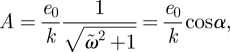
By setting |sin β| = 1, equation (4.9) yields

5.1

We note equations (3.9) and (3.11); and thus, and . In order to obtain a good measure of the mileage, we must look at the energy budget of the system. Integration of the elastic energy density (κ/2)(u_s − e)² over a distance λ yields a constant, because both u and e have the same wavelength λ and the same phase velocity v:

By partial integration, we obtain

5.2

This relationship represents the balance between the viscous dissipation rate (the left-hand side) and the energy input rate (the right-hand side) resulting from the active change of e (note that κ(u_s − e) is the internal tension). Thus, the integrand on the right-hand side, denoted by , represents the power density (J (s m)⁻¹). The spatial average of is calculated as

5.3

In the left-hand (approximate) equality above, we set u_s ≈ u_s⁽⁰⁾ ignoring errors of the order of O(ɛ¹). We introduce a ‘mileage’ quantity M (m (J m⁻¹)⁻¹) as follows:

5.4

Here, M represents the distance moved for one unit of energy density,³ thus large M implies low energetic cost for movement.

From equations (5.1) and (5.4), we obtain the result that

5.5

This indicates an inversely proportional relationship between |V| and M: no matter how the variables e₀, k and ω are adjusted, the time and energy efficiencies cannot be improved simultaneously.

5.2. Matching between diffusion dynamics and endogenous action

We now investigate the behaviour of |V| and M as functions of e₀, k and ω, by fixing κ and η₀ (and thus D₀). Note that e₀, ω and k characterize the endogenous action of e(s,t) (see equation (3.5)), whereas κ and η₀ can be regarded as material and environmental parameters.

Figure 4 shows plots of |V| and M versus e₀, ω and k (see equations (5.1) and (5.4)). In each plot, all other variables are set to unity. The following three results are apparent.

• — Dependence on e₀: we see that |V| ∝ e₀ and M ∝ 1/e₀ (figure 4a). The former relationship reflects the fact that we study a linear system that transforms an input function e(s,t) into an output function u(s,t), thus the amplitude of u is proportional to that of e. The e₀ dependence of |V| is inherited from u. The latter relationship arises because (while |V| ∝ e₀). The divergence of M for e₀ → 0 implies that if the system is allowed to spend an infinitely long time (|V| → 0 as e₀ → 0), it can move with an infinitely small energy cost. This non-dissipative behaviour for e₀ → 0 can be regarded as a quasi-static limit.

• — Dependence on ω: we see that , namely, that |V| ∝ ω for small ω, but |V| saturates at an upper limit for large values of ω (figure 4b). The crossover between these two types of behaviour occurs at approximately , i.e. when ω = k²D₀. This indicates that the frequency ω should be matched to (the inverse of) the diffusion time k²D₀ in order to achieve high time efficiency, but too high a frequency ω is of no use to the organism. As in the case of the e₀ dependence of M, the divergence of M for ω → 0 corresponds to a quasi-static limit.

• — Dependence on . As seen in figure 4c, the relationship between |V| and k reaches a maximum when (D₀k²)/ω = 1 is satisfied, corresponding to matching between the wavelength (∝ 1/k) and the diffusion length ().

Figure 4.

(a–c) Plots of |V| and M versus e₀, ω and k based on equations (5.1), (3.9), (3.11) and (5.4). (d) Surface plot of |V| (ω,k). (e) Surface plot of |V| (ω,k) for the case where the inertial effect is involved. In each plot, all other variables are set to unity.

Figure 4d shows a three-dimensional plot of |V| as a function of ω and k (all other parameters are set to unity). The ‘ridge’ corresponds to the condition of ω = k² (the matching condition for D₀ = 1). For comparison, we also provide a three-dimensional plot of |V| versus ω and k for the case where the inertial effect is involved (figure 4e; see §6.3).

We note that owing to the inversely proportional relationship between |V| and M, the most time-saving mode of locomotion is also the most energy-consuming mode (the minimum of M in figure 4c). That is to say, in this case it is true that time is money.

6. Discussion

6.1. Criterion to determine direction of peristaltic locomotion

The essential point of our theoretical analysis is summarized in figure 2b, from which we can extract the following two-step criterion for the direction of peristaltic locomotion. In the first step, we consider a virtual anchorless state. The peristaltic movement gives rise to a periodic velocity field along the system, which corresponds to u_t⁽⁰⁾(s,t) in the diffusion equation model. In the second step, we introduce anchors. If the anchors are placed at the points that had a negative velocity in the anchorless state (the term ‘negative’ represents being opposite to the wave propagation), the locomotion occurs into the positive direction, because the anchors cut down the negative velocity component. Another picture for the anchoring effect is that the anchored points pull/push neighbouring parts into the positive direction. This picture is clear and reasonable from a mechanical viewpoint; we can expect that the two-step criterion qualitatively applies to wider cases, regardless of details of friction law. To demonstrate the generality of the criterion, we consider the locomotion of myriapods [3] below.

Figure 5 schematically represents side views of a myriapod. Figure 5a shows a virtual anchorless state where the body of the myriapod is lifted up from the ground. We assume that the swing angle ϕ, defined in the right illustration in figure 5a, changes in the form of a sinusoidal wave travelling rightward: ϕ(n,t) = ϕ₀ sin(ωt − qn), where n is the number assigned to legs and q is the wavenumber with respect to n. We introduce the lateral displacement of the foot u(n,t) = L₀ sin ϕ, as shown in the right illustration (L₀ is the length of the legs in the side view). u(n,t) corresponds to u⁽⁰⁾(s,t) in the viscous friction model. For legs P and Q, u(n,t) = 0. By adequately choosing the origin of t, we can set (ωt − qn) = 0 for P and (ωt − qn) = −π for Q; thus, the lateral velocity of the foot v_foot = u_t(n,t) = ωL₀ϕ₀ cos ϕ sin(ωt − qn) is positive for P and negative for Q. Then, we consider the anchor. If the foot of Q contacts the ground with non-slip condition while the foot of P is lifted up from the ground by changing the joint angles of the leg (see the right illustration representing a cross-sectional view), the main body is driven into the positive direction, opposite to v_foot of the leg Q in the anchorless state. Note that the feet of P and of Q exist in regions where the feet density is high and low, respectively. The argument here is essentially identical to what figure 2b explains.

Figure 5.

Illustrations to consider the kinematics of locomotion of myriapods. (a) Virtual anchorless (frictionless) state. The swing angle ϕ and lateral displacement of foot u are defined in the rightward illustration. (b) Rightward movement of the entire body by the anchored leg of Q. The leg P is lifted up by changing joint angles (the rightward illustration).

Here, we insert a brief comment on the anisotropic friction. The importance of anisotropic friction is emphasized in some literatures [4,15–18]. For example, bristles of earthworm tilt to increase frictional resistance to backward sliding. Indeed, when the friction is anisotropic, internal peristaltic movement is automatically converted into directional locomotion without active anchor control. This is because of the following reasons: in the virtual anchorless state (e.g. the state where the system is lifted up from the substrate), the internal peristaltic movement makes some parts move into the direction of the stronger friction. When the system returns onto the substrate, the parts automatically serve as anchors owing to the stronger friction. According to our criterion, the system moves into the direction of weak friction. A shortcoming of this manner of locomotion is that the direction of locomotion is fixed from the beginning, and thus the crawler cannot undergo backward movement even though it reverses the direction of the peristaltic wave. At the best of author's knowledge, it is not clear where there exists any real peristaltic crawler that undergoes directional locomotion using only anisotropic friction (without the active control of the friction). For the case of earthworm, the anchor position is actively changed by cycles of poking and retracting the bristles. At least, if a peristaltic crawler undergoes an active control of the anchor position coordinated with peristaltic wave propagation, the friction does not have to be anisotropic.

6.2. Consideration on rigid machinery limit

Equation (4.9), the criterion that determines the direction of locomotion, is an approximative relationship of the order of O(ɛ). For the relationship to apply with high accuracy, the anchoring intensity (or perturbation parameter) ɛ must be so small that the anchor does not disturb the internal deformation. In contrast, if the springs in figure 1b are replaced by rigid rods and the action that changes the opening angle of the hinges is powerful enough, the internal deformation of the system (i.e. the relative displacement between adjacent blocks) is not affected by the frictional force on the blocks. In this ‘rigid machinery’ limit, we expect that a relationship essentially equivalent to equation (4.9) will hold as an exact condition, regardless of the intensity of the anchoring. Below, we consider the rigid machinery limit, and show that this expectation is correct.

In the continuous description, the rigid machinery limit is characterized by κ → ∞ and u_s = e(s,t). This implies that the strain field u_s can follow e with no phase delay. Instead of equation (3.6), we have

6.1

where the tension T(s,t) is an undetermined function. We employ equation (3.5) and the following expression for η(s,t):

6.2

and

6.3

We note that q(s,t) does not include the parameter α indicating a phase delay between e(s,t) and u_s(s,t), and that the intensity of anchoring, μ > 0, is arbitrary. From u_s = e = e₀ sin(ω t − ks),

6.4

where U(t) represents the component of uniform translation. Because we can assume that T(s,t) has a period of λ, the spatial average of both sides of equation (6.1) gives 〈ηu_t〉_λ = 0. By substituting equations (6.2)–(6.4) into equation 〈ηu_t〉_λ = 0 and rearranging the terms, we obtain U′(t) = (e₀ω/k)〈η(s,t) sin(ωt − ks)〉_λ/〈η(s,t)〉_λ. Because η(s,t) = η(s − vt, 0) and η(s, 0) has the periodicity λ, we can set t = 0 in the above spatial averages, which indicates that the translational velocity U′(t) is independent of t (hence can be denoted by V). By performing the spatial integration of the average, we obtain

6.5

Here, |V| increases with increasing anchoring intensity μ, and saturates at an upper limit of e₀v sin β as μ → ∞. Because e₀ < 1 (see the discussion below equation (3.5)), the locomotion speed V cannot be faster than the phase velocity v.

6.3. Applicability of the model to different friction modulations

We have investigated the effect of localized anchoring on directional locomotion by formulating a linear perturbation model expressed in equations (4.1)–(4.7). Owing to the linearity of our model, the results obtained in §4 can be applied to different types of modulation of the friction coefficient. If the sign of the friction pulse is flipped such that p(s,t) → −p(s,t), the sign of V (and thus the criterion for the locomotion direction) is reversed. This follows from the fact that 〈u⁽¹⁾〉_λ depends linearly on p(s,t) (see equation (4.4)). The locomotion expressed by the negative pluses can be described in the following manner. Almost all parts of the body are anchored, but the anchor is locally weakened at the points where the negative pulses are located, which allows faster sliding of the points. The directional motion of the system as a whole is determined by the localized sliding of these released points.

Thus far, we have assumed that only one pulse exists in an interval of the length λ in s-space. Our calculations can be extended to the case where the interval includes m pulses; the friction coefficient is then given by η(s,t) = η₀(1 + ɛP(s,t)), where (here we have explicitly represented the β-dependence of p). The factor f_j (which can be negative) is the intensity of the pulse with phase shift β_j(0 ≤ β_j < 2π). Because of the linearity, the average velocity in this multi-pulse case is , where V(β ) = −ɛωA sin β is the average velocity in the single pulse case (equation (4.9)).

An analogous calculation is possible for the case in which the perturbation P is given by a continuous function with spatial period λ and phase velocity v = ω/k, that is, P = P(s,t;α) = f(ks − (ωt − α)), where f(·) is a 2π-periodic function. Noticing that f(ks − (ωt − α)) = (2π)⁻¹ ∫₀^2π dβ f(β) p(s,t;β), we can calculate the average velocity V_f by . For example, if f(β) = sin(β − γ), we obtain V_f ∝ (−1)cosγ: the direction of locomotion is determined by the phase shift γ that indicates the extent of overlap between the two sine functions f(β) and sin β. We note that V_f > 0 if γ satisfies the condition π/2 <γ < 3π/2 (i.e. if a peak in f(ks) = sin(ks − γ) exists in the interval λ /2 < s < λ). This condition corresponds to that of the single pulse case in figure 2b, that is, V > 0 if the δ-pulse exists in the interval λ/2 < s < λ.

The idea of perturbative treatment for friction modulation can apply to different situations. For example, it is interesting to ask how the randomness of the environment (i.e. the condition of the substrate) affects locomotion. This problem can be treated by including a random position function R(X) = R(s + u) in the perturbation function, such that P(s,t) = f(ks − (ωt − α)) + R(s + u). Here we impose, for example, the white noise condition of 〈R(y)〉_s = 0 and 〈R(y)R(y + z)〉_s ∝ δ(z) (the subscript ‘s’ represents the statistical (or long-distance spatial) average). The statistical average of 〈u_t⁽¹⁾〉_s determines the mean velocity of locomotion.⁴

6.4. Consideration of inertial and dry friction effects

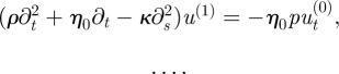
A major simplification of our model is that we have neglected inertial effects and dry friction. We now briefly discuss these factors. Inertial effects can be included in our model by including the inertial term ρu_tt (ρ is the line density) in the left-hand side of equation (3.4). When η(s,t) includes a weak modulation, the governing equation for the system is

6.6

The system has two characteristic timescales of (the inverse of) the diffusion time ω_d and the eigenfrequency ω_c defined by

6.7

where is the velocity of the elastic wave. For convenience of the description below, we introduce a dimensionless parameter

6.8

The perturbation expansion of equation (6.6) yields

6.9

and

6.10

Since u_s⁽¹⁾ is expected to have the same spatial period λ as e(s,t) and u⁽⁰⁾, the average velocity V can be calculated in the manner completely parallel to the case without the inertial term. The travelling-wave solution of u⁽⁰⁾ is

6.11

6.12

and

6.13

Averaging both sides of equation (6.10) yields 〈u_t⁽¹⁾〉_λ =−〈p(s,t)u_t⁽⁰⁾(s,t)〉_λ, because we have (i.e. the λ-periodicity of u_t⁽¹⁾ provides a constant value of 〈u_t⁽¹⁾〉_λ). When p is given by an array of δ-function, we obtain 〈u_t⁽¹⁾〉_λ = −ωAsin β and V = −ɛ ωAsin β. For optimal anchoring (| sin β | = 1), |V| is given by

6.14

If we regard |V| as a function of ω fixing other parameters, it reaches a maximum of

6.15

for

6.16

We note that equation (6.16) is the condition for occurrence of the resonance between the elastic oscillation and the endogenous action. Equation (6.15) shows that the maximum velocity is proportional to the diffusion coefficient D₀. Figure 4e shows a three-dimensional plot of |V| as a function of ω and k (all other parameters including r are set to unity). In the present case, including the inertial effect, both a cross section of |V| (ω, k) at a constant k and that at a constant ω have a maximum.

In contrast, dry friction is a strongly nonlinear effect. The addition of a new term describing dry friction violates the linearity of our equations of motion and makes them much harder to deal with. In other words, the behaviour of the system becomes more complex, especially, if inertial effects are also included (e.g. a new oscillatory mode caused by stick–slip instability should be involved). Although detailed analysis of the nonlinear equations of motion is beyond the scope of this paper, it is at least possible and informative to make a comparison with the simple kinematic model discussed by biologists [5,9], in which dry friction dominates the locomotion dynamics.

In this model, the body of a peristaltic crawler is represented by a one-dimensional array of blocks (figure 3b). Each block (corresponding to a body segment) adopts either an elongated or contracted state; contracted blocks become thicker and are prevented from sliding along the ground by dry friction, whereas elongated (thin) blocks are lifted up from the ground and are able to move freely in the lateral direction. The body as a whole is assumed to adopt a periodic domain structure consisting of alternating sequences of N_c consecutive contracted blocks and N_e consecutive elongated blocks. When the elongation–contraction wave propagates towards the right, the system as a whole moves in the opposite direction, as seen in figure 3b. Although the basic picture of the kinematic model is fairly different from ours, the same prediction for the locomotion direction is obtained: anchoring contracted parts of the body gives rise to locomotion opposite to the direction of wave propagation. Therefore, we expect that although our model is based on a particular (simple) friction law, the qualitative aspects of the predictions that it yields are generic (see §6.1).

7. Concluding remarks

We close this paper with the following concluding remarks. In the first paragraph of §1, we stated that peristaltic crawlers break forwards–backwards symmetry. Here, we emphasize that much attention should be paid to the character of the symmetry breaking. In the two-block model with no anchor control and in the continuum model with uniform η, backwards–forwards symmetry is clearly broken (i.e. for an arrangement of two blocks with different viscous friction coefficients and for the propagation of an elongation–contraction wave). However, no directional motion occurs. On the other hand, anisotropic friction seems somewhat excessive; it inhibits backward motion (when the same head direction is maintained). Most real crawling organisms seem to adopt a more moderate process involving the active spatio-temporal control of friction. In this paper, we have considered an essential aspect of the friction control, based on a simple mechanical model describing one-dimensional locomotion driven by peristaltic wave propagation. From analytical treatments of the proposed model, we extracted a two-step criterion for locomotion direction. In the first step, we consider a virtual anchorless (or frictionless) state, and look at the distribution of local velocity produced by internal motion. In the second step, we make anchors at parts of which local velocities (in the anchorless state) point a particular direction; the formation of the anchors results in locomotion into the opposite direction. The basic idea of this criterion would apply to various cases other than the one-dimensional peristaltic locomotion, for example, the locomotion of ear shell for which the two-dimensionality of contact area cannot be ignored [1,3]. We expect the insight obtained in this paper will be helpful to understand a wide class of limbless locomotion.

Appendix A

As a result of the perturbative treatment of equation (4.1), we encounter a series of diffusion equation with a diffusion constant D₀ and source term. The (formal) solution of f_t = D₀ f_ss + g(s,t) can be obtained by the following formula:

A 1

where

A 2

is the Gaussian Green's function. In equation (4.3), f = u⁽¹⁾ and g = −pu_t⁽⁰⁾. Substituting equations (3.8) and (4.6) into this formula, we obtain

A 3

where Δu⁽¹⁾ = u⁽¹⁾(s,t) − u⁽¹⁾ (s,0), C = −λωA sin(kβ) and B_n = B + nλ − α/k. We note that owing to the infinite sum with respect to n, u⁽¹⁾(s,t) has the spatial period of λ if u⁽¹⁾(s,0) has the same special period.

Since for any f(s), the spatial average of Δu⁽¹⁾ is given by

A 4

The integration about s yields unity because the integrand is a normalized Gaussian function. Thus, we reproduce

References

- 1.Lissmann H. W. 1945. The mechanism of locomotion in gastropod molluscs. I. Kinematic. J. Exp. Biol. 21, 58–69 [DOI] [PubMed] [Google Scholar]
- 2.Wells M. 1968. Lower animals. London, UK: George Weidenfeld and Nicolson Ltd [Google Scholar]
- 3.Gray J. 1968. Animal locomotion. London, UK: George Weidenfeld and Nicolson Ltd [Google Scholar]
- 4.McNeill Alexander R. 1992. Exploring biomechanics: animals in motion. New York, NY/Oxford, UK: Freeman and Company [Google Scholar]
- 5.McNeill Alexander R. 2002. Principles of animal locomotion, pp. 86–90 and pp. 166–180 Princeton, NJ/Oxford, UK: Princeton University Press [Google Scholar]
- 6.Quillin K. J. 1999. Kinematic scaling of locomotion by hydrostatic animals: ontogeny of peristaltic crawling by the earthworm lumbricus terrestris. J. Exp. Biol. 202, 661–674 [DOI] [PubMed] [Google Scholar]
- 7.Zimmermann K., Zeidis I., Behn C. 2009. Mechanics of terrestrial locomotion-with a focus on non-pedal motion systems. Berlin/Heidelberg, Germany: Springer [Google Scholar]
- 8.Heffernen J. M., Wainwright S. A. 1974. Locomotion of the holothurians Euapta lappa and redefinition of peristalsis. Biol. Bull. 147, 95–104 [Google Scholar]
- 9.Elder H. Y. 1985. Peristaltic mechanism. In Aspects of animal movement (eds Elder H. Y., Trueman E. R.), pp. 71–92 Cambridge, UK: Cambridge University Press [Google Scholar]
- 10.Denny M. W. 1980. The role of gastropod pedal mucus in locomotion. Nature 285, 160–161 10.1038/285160a0 (doi:10.1038/285160a0) [DOI] [Google Scholar]
- 11.Denny M. W., Gosline J. M. 1980. The physical properties of the pedal mucus of the terrestrial slug, Ariolimax columbianus. J. Exp. Biol. 88, 375–393 [Google Scholar]
- 12.Lauga E., Hosoi A. E. 2006. Tuning gastropod locomotion: modeling the influence of mucus rheology on the cost of crawling. Phys. Fluids 18, 113102. 10.1063/1.2382591 (doi:10.1063/1.2382591) [DOI] [Google Scholar]
- 13.Rieu J.-P., Barentin C., Maeda Y., Sawada Y. 2005. Direct mechanical force measurements during the migration of Dictyostelium slugs using flexible substrata. Biophys. J. 89, 3563–3576 10.1529/biophysj.104.056333 (doi:10.1529/biophysj.104.056333) [DOI] [PMC free article] [PubMed] [Google Scholar]
- 14.Lin H.-T., Trimmer B. A. 2010. The substrate as a skeleton: ground reaction forces from a soft-bodied legged animal. J. Exp. Biol. 213, 1133–1142 10.1242/jeb.037796 (doi:10.1242/jeb.037796) [DOI] [PubMed] [Google Scholar]
- 15.Mahadevan L., Daniel S., Chaudhury W. K. 2004. Biomimetic ratcheting motion of a soft, slender, sessile gel. Proc. Natl Acad. Sci. USA 101, 23–26 10.1073/pnas.2637051100 (doi:10.1073/pnas.2637051100) [DOI] [PMC free article] [PubMed] [Google Scholar]
- 16.Miller G. S. P. 1988. The motion dynamics of snakes and worms. ACM SIGGRAPH Comp. Graph. 22, 169–173 [Google Scholar]
- 17.Menciassi A., Accoto D., Gorini S., Dario P. 2006. Development of a biomimetic miniature robotic crawler. Auton. Robot. 21, 155–163 10.1007/s10514-006-7846-9 (doi:10.1007/s10514-006-7846-9) [DOI] [Google Scholar]
- 18.Zimmermann K., Zeidis I. 2007. Worm-like locomotion as a problem of nonlinear dynamics. J. Theoret. Appl. Mech. 45, 179–187 [Google Scholar]