Detecting genome-wide epistases based on the clustering of relatively frequent items

Abstract

Motivation: In genome-wide association studies (GWAS), up to millions of single nucleotide polymorphisms (SNPs) are genotyped for thousands of individuals. However, conventional single locus-based approaches are usually unable to detect gene–gene interactions underlying complex diseases. Due to the huge search space for complicated high order interactions, many existing multi-locus approaches are slow and may suffer from low detection power for GWAS.

Results: In this article, we develop a simple, fast and effective algorithm to detect genome-wide multi-locus epistatic interactions based on the clustering of relatively frequent items. Extensive experiments on simulated data show that our algorithm is fast and more powerful in general than some recently proposed methods. On a real genome-wide case–control dataset for age-related macular degeneration (AMD), the algorithm has identified genotype combinations that are significantly enriched in the cases.

Availability: http://www.cs.ucr.edu/~minzhux/EDCF.zip

Contact: minzhux@cs.ucr.edu; jingli@cwru.edu

Supplementary information: Supplementary data are available at Bioinformatics online.

1 INTRODUCTION

With recent development in high-throughput single nucleotide polymorphism (SNP) genotyping technologies, the number of SNPs that can be typed simultaneously on a DNA chip has grown from 10 000 in 2002 to 1 million in 2007 (Altshuler et al., 2008). Genome-wide genotype data as well as phenotype information for some common diseases have been accumulated in an accelerated rate for the past 5 years (e.g. Melum et al., 2011; Stuart et al., 2010; WTCCC, 2007). These genome-wide association studies (GWASs) have proven to be a powerful approach to reveal susceptibility genes for some complex diseases (Goldstein, 2009; Hardy and Singleton, 2009). Nevertheless, the primary analysis paradigm for GWAS is dominated by single locus-based statistical approaches (He and Lin, 2011). However, epistatic interactions (epistases) among multiple genes play an essential role in the pathogenesis of human complex diseases (Cordell, 2009; Phillips, 2008). Many studies have also demonstrated that epistasis contributes to diseases such as breast cancer (Ritchie et al., 2001), diabetes, obesity (Cordell, 2009) and coronary heart disease (Nelson et al., 2001). Single locus-based approaches may not be able to detect all interacting genes, especially for those with small marginal effects.

Recently, the problem of detecting genome-wide epistases has drawn much attention. Many computational algorithms have been proposed (Cordell, 2009; Li et al., 2011a, b; Moore et al., 2010; Tang et al., 2009; Wan et al., 2010a, b, c; Zhang and Liu, 2007). Existing approaches for searching gene–gene or SNP–SNP interactions can be grouped into four broad categories: exhaustive search, stochastic search, data mining/machine learning approaches and stepwise search. Methods based on exhaustive search enumerate all possible combinations of multiple loci and perform desired interaction tests (e.g. χ² or logistic regression) for each combination. Nelson et al. (2001) proposed a combinatorial partitioning method (CPM), which searches all possible ways of dividing m-locus genotype combinations into k genotypic partitions, and selects the best one to account for quantitative traits. CPM is only computationally feasible for small datasets even for two-locus interactions due to the enormous number of possible partitions. Inspired by CPM, Ritchie et al. (2001) proposed a multifactor-dimensionality reduction method (MDR), which partitions the multi-locus genotype space into two classes and exhaustively searches for the best classification model in predicting the disease status. It utilizes repeated cross-validations and permutation tests to evaluate classification accuracy and significance, respectively. Similar to CPM, MDR cannot handle large datasets, even for two-locus interactions (Cordell, 2009). Though many extensions of MDR have been proposed recently, including MB-MDR (Cattaert et al., 2011) and RMDR (Gui et al., 2011), they are unable to tackle large GWAS data efficiently. In another attempt, Wan et al. (2010c) proposed a boolean operation-based screening and testing (BOOST) method, which can detect two-locus interactions for currently available GWAS data. However, because the search space grows exponentially with the number of involved genes/SNPs, methods based on exhaustive search can hardly be extended to include more than two loci.

Instead of explicitly enumerating all possible combinations of m-locus, stochastic methods (Li et al., 2011a; Tang et al., 2009; Zhang and Liu, 2007) use random sampling procedures to search the space of interactions. Among them, Bayesian epistasis association mapping (BEAM) (Zhang and Liu, 2007) is one of the representatives. BEAM takes case–control genotypes as its input, and iteratively uses the Markov chain Monte Carlo (MCMC) approach to calculate the posterior probability of a locus being associated with the disease and/or being involved with other loci in epistasis. Tang et al. (2009) further extended BEAM in their epistatic module detection (epiMODE) method, which uses Gibbs sampling and a reversible jump MCMC procedure to search for significant epistatic modules.

Data mining and machine learning approaches, such as neural networks (Ritchie et al., 2003), random forests (Schwarz et al., 2010), boosting (Li et al., 2011b) and predictive rule learning algorithms (Wan et al., 2010b), have all been used in search for significant interactions. Most of these algorithms use some heuristics to avoid exhaustive searches. For example, SNPruler (Wan et al., 2010b) first uses a rule searching algorithm to find potential interactions and then adopts the χ² statistic to evaluate their significance. Stepwise search approaches first select a subset of SNPs based on some single-locus tests (or measures); tests for multi-locus interactions are then conducted based on the subset of SNPs detected in the first step (Li, 2008; Marchini et al., 2005). Comparing to exhaustive approaches, stepwise algorithms usually are much faster, and may perform reasonably well for diseases with some marginal effects. On the other hand, stepwise search procedures may not be able to find interactions involving loci with small or no marginal effects. Similarly, methods based on stochastic search or machine learning algorithms cannot guarantee to find all significant interactions.

In this article, we propose an algorithm called Epistasis Detector based on the Clustering of relatively Frequent items (EDCF) to detect multi-locus epistatic interactions in case–control studies. EDCF adopts the stepwise search strategy and starts with two-locus interaction models. It groups all genotype combinations into three clusters, representing frequent genotypes in cases, frequent genotypes in controls and the remaining genotypes. Items in the three groups for higher order interactions are then constructed sequentially. The significance of the final partitions can be evaluated by Pearson's χ² test. Extensive experiments on simulated data show that EDCF is faster and more powerful, in general, in finding the epistatic interactions than some of the recently proposed methods including MB-MDR, BOOST, SNPRuler and epiMODE. By applying the algorithm on a real genome-wide case–control data set for age-related macular degeneration (AMD), some genotype combinations have been found that are significantly enriched in the cases.

2 METHODS AND MATERIALS

2.1 Notations

We assume all SNPs are diallelic and a genotype is encoded as 0, 1 or 2 according to the number of copies of the minor allele present at each SNP locus. For example, suppose A is the major allele and a is the minor allele at SNP locus A. The genotype A/A, A/a and a/a are encoded as 0, 1 and 2, respectively. For a case–control GWAS study, given the genotype data at M SNPs of N individuals with their dichotomous disease status, we use S to denote the ordered set of the M SNPs, s_i to denote the i-th SNP in S, f_m(s_i) to denote the minor allele frequency at s_i and g_i(j) to denote the genotype of the j-th individual at s_i.

Let N^a and N^u denote the number of affected individuals (i.e. cases) and the number of normal individuals (i.e. controls), respectively. Let (v₁,…, v_d) be a d-locus genotype combination at s_i1,…, s_id. Let n^a_v1,…,vd and n^u_v1,…,vd be the number of affected and unaffected individuals with genotypes (v₁,…, v_d) at loci s_i1,…, s_id, respectively. Let n^t_v1,…,vd=n^a_v1,…,vd+n^u_v1,…,vd. Let f_v1,…,vd denote the population frequency of (v₁,…, v_d), which can be obtained based on genotype frequencies at each locus when assuming linkage equilibrium among all the involved loci. Let p_{v1,…, vd} denote the penetrance of (v₁,…, v_d) (i.e. the probability of being affected given the genotype combination). The population prevalence p can then be calculated as:

(1)

2.2 Genotype combination clustering

The primary goal of association analysis is to find SNPs with allele and/or genotype frequencies in cases that are significantly different from those in controls. Many factors, including effect size, allele frequency, linkage disequilibrium between markers and disease loci, as well as sampling errors, may affect the distribution. The underlying assumption is that at the disease loci, the penetrance of their genotype combinations has drastic differences (see Table 1 for an example.) One can view the genotype combinations with penetrance greater than the population prevalence as high-risk combinations, as shown in bold with grey background in Table 1, while the others are regarded as low-risk combinations. However, in practice, one cannot directly use the assumption because the true disease genes/SNPs as well as their penetrance tables are unknown. Instead, we have to rely on the observed distributions of genotype combinations in cases/controls, usually organized in a contingency table (e.g. Table 2). A popular program, MDR (Ritchie et al., 2001) adopts a simple strategy in defining high/low-risk genotype combinations, by comparing the case/control ratio of each genotype combination with the overall case/control ratio. However, because of random sampling errors, this simple method may not work well in practice, especially with combinations whose case/control ratio is close to the overall ratio (Park and Hastie, 2008) , as illustrated in Table 2. Therefore, MDR may fail to detect such interactions.

Table 1.

The penetrance table of an example two-locus interaction model

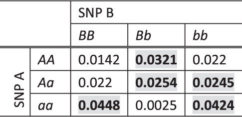Here, f_m(A)=f_m(B)=0.4 and the population prevalence P=0.024. The entries in bold with grey background are the high-risk two-locus genotype combinations, and the remaining are low-risk combinations.

Table 2.

A two-locus contingency table sampled from a population with the penetrance table in Table 1

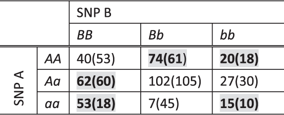Counts in controls are in the brackets. N^a=N^u=400. The entries in bold with grey background are the ones with ratios greater than N^a/N^u, therefore, regarded as high-risk combinations by MDR. And the others are low-risk combinations. The classification by MDR may not be consistent with the underlying penetrance (e.g. genotype combinations ‘AAbb’, ‘AaBB’, ‘AaBb’ and ‘Aabb’).

To prevent such cases, in this article, we propose to partition all genotype combinations into three groups, defined as G₀, G₁ and G₂, where G₀ contains all combinations that occur significantly more frequently in cases than in controls (presumably high-risk combinations); G₂ contains those occurring significantly more frequently in controls than in cases (presumably low-risk combinations); and G₁ contains the others. To do so, we first need to derive some thresholds for declaring significance. Considering a genotype combination (v₁,…, v_d) at d loci s_i1,…, s_id, under the null hypothesis that the penetrance p_{v1,…, vd} is the same as the population prevalence p, the number of cases n^a in the contingency table corresponding to (v₁,…, v_d) should follow a Binomial distribution n^a ~ B(n=n^t, p_a=N^a/(N^a+N^u)). (For brevity, we omit the subscript ‘v₁,…, v_d’ from the notations in this section when it is implied in the context.) Similarly the number of controls n^u ~ B(n=n^t, p_u=N^u/(N^a+N^u)). For a given significance level α_s (e.g. α_s=0.05), let T_a denote the critical value corresponding to α_s for cases, i.e. Pr(k>T_a|n^t, p_a)<α_s. T_u is defined similarly for controls.

Definition 1. —

If n^a>T_a, (v₁,…, v_d) is a relatively frequent item under α_s in cases, and if n^u>T_u, (v₁,…, v_d) is a relatively frequent item under α_s in controls.

Based on the above definitions, for a given α_s and for a set of SNPs, we define G₀ as the set of relatively frequent items in cases, G₂ as the set of relatively frequent items in controls, G₁ as the set of all other genotype combinations.

2.3 Evaluation of interactions

Once all genotype combinations of d SNPs have been grouped into G₀, G₁ and G₂, a 3×2 contingency table (Supplementary Table S1) can be easily obtained, where the rows are the three groups and the columns are cases and controls. The χ² statistic with 2 degrees of freedom (Fisher, 1922), denoted as X²₂(i₁,…, i_d) here, can be used as a measure of significance for the partition. Intuitively, a group of SNPs with high X²₂ may represent a group of interacting SNPs. However, this is not always true, because it is possible that some SNPs in the group might be redundant (e.g. when they do not affect the assignment of the three groups). To avoid such cases, we define an interaction module as a smallest possible significant SNP subset.

Definition 2. —

If the following conditions are satisfied, (s_i1,…, s_id) is an interaction module under the significance level α:

1. the P-value of X²₂(i₁,…, i_d)≤α;

2. there is no subset {i′₁,…, i′_d′}(d′<d) of {i₁,…, i_d} such that X²₂(i′₁,…, i′_d′)≥X²₂(i₁,…, i_d).

When there are many interaction modules, biologists may only be interested in the k most significant ones. In the next subsection, we propose an algorithm called EDCF to find the top-k significant genome-wide multi-locus interaction modules for a given d.

2.4 Algorithm

We develop an iterative algorithm to search for the top-k significant d-locus interaction modules. The numbers of SNPs in current GWAS range from several hundreds of thousands to a few millions. For interactions involving d (d≥3) loci, it is impractical to exhaustively search the whole space. In order to obtain the top-k significant d-locus interaction modules, we first obtain the top-kf_s significant (d−1)-locus interaction modules (where f_s≥1 is a scale factor), with the assumption that some subsets of a significant interaction module will also be ranked high. The algorithm recursively searches the interaction space with smaller numbers of SNPs until d reaches 2, in which case all 2-locus genotype combinations will be evaluated. We stop at 2-locus interactions, because with an efficient implementation it is feasible to examine all pairwise SNPs for current GWAS. The significance of interaction modules is evaluated based on the X²₂ statistic defined earlier, with appropriate adjustments for multiple testing (see next subsection). An efficient implementation of the algorithm, which takes advantage of bitwise operations (Wan et al., 2010c) and a binary minimum heap structure, is available from the first author's website. The details of the algorithm and the analysis of its properties can be found in the Supplementary Material.

2.5 Type I error control

A challenge in epistasis analysis for GWAS is to appropriately control type I errors in the presence of multiple comparisons. Permutation tests and Bonferroni corrections are the two commonly used approaches for correcting the multiple testing problem. For EDCF, there are two levels of comparisons. The first level is due to the fact that there are d-locus combinations for a dataset with M SNPs. The second is related to the following fact. For d loci, EDCF clusters the 3^d possible genotype combinations into three groups and conducts the χ² test with 2 degrees of freedom. When d increases, even if the data were generated randomly, the χ² statistic will increase obviously because of the non-random clustering of d-locus genotype combinations. In theory, there are 3^3d possible ways to cluster 3^d genotype combinations into three groups. Considering the number of clustering patterns in practice is far less than 3^3d, the simple Bonferroni correction [i.e. dividing the significant level by ] is too conservative for EDCF. However, permutation tests are time consuming when M is large.

To properly control type I error (i.e. false positive) rates of EDCF in an efficient way, we propose to combine Bonferroni correction with permutation tests. Considering that the two levels of multiple tests are independent, we use Bonferroni correction to control the first level and use permutation tests to control the second level multiple tests. More specifically, the overall significant level is defined as:

(2)

where corresponds to the Bonferroni correction for multi-locus combinations and α₀ can be chosen from permutation tests for different d values on small datasets to ensure the overall significant level at 0.05.

2.6 Experimental design

To evaluate the effectiveness of EDCF, we perform extensive simulation experiments using different disease models and compare its power with that of some recently proposed approaches including MB-MDR (Cattaert et al., 2011), BOOST (Wan et al., 2010c), SNPruler (Wan et al., 2010b), epiMODE (Tang et al. 2009), as well as the naive 2-locus χ² test (ChiSQ). The procedure to generate background SNP genotypes is the same as the one used in previous studies (e.g. Wan et al., 2010c). For each SNP s_i, its minor allele frequency f_m(i) is first sampled uniformly at random from [0.05, 0.5]. Then the genotype g_i(j) of an individual j is generated based on the allele frequency by assuming Hardy–Weinberg equilibrium. Finally, the genotypes at the disease loci for cases and controls are generated according to disease models, which will be described in next subsection.

2.6.1 Disease models

In our simulation experiments, we consider two types of disease models: epistasis models with and without marginal effects, and consider interactions with two or three SNPs. A disease model can be defined either by specifying the penetrance table [i.e. p_{v1,…, vd} for a genotype combination (v₁,…, v_d)] or by specifying the odds table. The odds of a genotype combination (v₁,…, v_d) is defined as

(3)

In theory, one can arbitrarily assign a penetrance (or odds) value to a genotype combination. In practice, many researchers only focus on constrained models. In many cases, there are only two free parameters, one representing baseline effect and the other representing additional effect relative to the baseline (e.g. Supplementary Tables S2 and S5). Even with two parameters, it is still hard to directly assign their values. Instead, one usually can specify the population prevalence p and another factor (either genetic heritability or marginal effect), and then numerically solve the two free variables based on their relationship for a given disease allele frequency. The genetic heritability h² is defined as Culverhouse et al. (2002)

(4)

The definition of the marginal effect size λ of a disease locus is the same as the one used in Zhang and Liu (2007).

(5)

Once the penetrance/odd table is resolved, the conditional genotype distribution given a disease status can be calculated and genotypes of cases and controls at these loci can be generated accordingly.

For two-locus models with small marginal effects, we consider Models 1–4 (Supplementary Table S2). Model 1 involves two-locus multiplicative effects (Marchini et al., 2005). Model 2 is model Ep-6 in Neuman and Rice (1992), which has been used as a model for handedness and the color of swine. Model 3 corresponds to model M86 in Li and Reich (2000) and Model 4 is a well-known XOR model (Li and Reich, 2000). The same models have also been used in previous studies (Wan et al., 2010c). For a fixed minor allele frequency f_m of a disease−associated SNP, the parameters β and θ of Models 1–4 in Supplementary Table S2 can be solved based on the population prevalence p and genetic heritability h². For two-locus models without marginal effects, we choose the same 60 two-locus pure epistasis models (Supplementary Tables S3 and S4) as those in Wan et al. (2010) in our simulation study. For three-locus models, we consider one with marginal effect (Model 5 in Supplementary Table S5) and one without marginal effect (Model 6 in Supplementary Table S6). Model 5 has some marginal effects, which is essentially the same as Model 4 in Zhang and Liu (2007). To be consistent with the original paper Zhang and Liu (2007), we use the marginal effect size to control the disease effect of Model 5. Model 6 is proposed by (Culverhouse et al., 2002), which yields maximum genetic heritage h² with no marginal effect for the population penetrance p∈(0, 1/16] with minor allele frequency f_m=0.5.

To further evaluate the effect of linkage disequilibrium (LD) between markers and disease SNPs on the detection power of each approach, we consider two scenarios in our experiments. We either randomly insert the disease SNPs themselves into the background genotypes, or embed SNP markers of the same frequencies but in LD (r²=0.7) with the disease loci.

2.6.2 Statistical power

In comparing the performance of different algorithms, we adopt the same measure of discrimination power proposed by Wan et al. (2010b, c), which is defined as n_c/n, where n_c is the number of replicates in which the true interaction loci are detected by the algorithm and n is the total number of replicates. The true interaction loci are detected if the set is the most significant one and its P-value is smaller than the predefined threshold for all the programs except epiMODE. epiMODE does not output the significance levels of epistasis modules. Therefore, if there is a module in its output that contains and only contains the embedded loci, epiMODE is considered to be successful in detecting the true epistasis. Only algorithms that can explicitly output d-locus interactions on d-locus disease models are compared against one another. In our simulation study, we consider different sample sizes with the balanced design (i.e. N^a=N^u). For EDCF, we set α_s=0.05, k=20 and f_s=M/k unless otherwise stated.

3 RESULTS

We first discuss the control of false positive rates using simulated background genotype data, then compare the performances of EDCF, MB-MDR, BOOST, SNPruler, epiMODE and ChiSQ on different disease models. At last, we present the results of EDCF on a real GWAS dataset. The programs of MB-MDR (C++ implementation), BOOST (64 bit), SNPRuler and epiMODE are downloaded from the websites of their authors. Recall that MB-MDR is a recent extension of MDR, BOOST is a fast exhaustive search approach to detect two-locus interactions, SNPRuler uses rule inference and can deal with three-locus and higher order interactions, and epiMODE is a recent extension of BEAM using stochastic search. ChiSQ is the two-locus Pearson's χ² test with 8 degrees of freedom that is implemented in C++. All tests are conducted on a 64 bit Linux platform with 2.8 GHz CPU and 16 GB RAM. Unless otherwise stated, for each model and each parameter set, 100 replicates are randomly generated and each replicate contains 2000 SNPs.

3.1 False positive rate

We set the significance level and test EDCF on simulated genotype data without any disease loci embedded to obtain the false positive rate. One thousand datasets are generated and the false positive rate is defined as n_f/1000, where n_f is the number of datasets from which EDCF reports one or more interaction modules. Each dataset consists of 2000 SNPs (i.e. M=2000) and 800 individuals (400 cases and 400 controls). The test results (Fig. 1a) show that if α₀ is set 0.02 for d=2, 0.002 for d=3 and 0.00002 for d=4, the overall false positive rate of EDCF is <0.05. Therefore, in the following simulations, we let α₀=0.02, 0.002, 0.00002 for d=2, 3, 4, respectively, to control the overall false positive rate of EDCF.

Fig. 1.

False positive rates under the null model. The plot in (a) shows the false positive rates of EDCF using different α₀s for different ds, and the plots in (b) and (c) show the false positive rates of EDCF and BOOST when the sample size (b) and the number of SNPs (c) vary.

To properly control the false positive rates for programs MB-MDR, BOOST, SNPruler and epiMODE, we mainly follow the recommendations from the original authors while considering the number of SNPs (mostly 2000 SNPs in our tests). MB-MDR uses permutation tests to control type I errors and its significance level is set to be 5%. By default, BOOST outputs all two-loci interactions with τ≥30 (definition see Wan et al., 2010c), which corresponds to an unadjusted P ≤4.89×10⁻⁶. SNPRuler outputs the top-k rules that contain d loci (k is set to be 20 in the following tests). The rules are then filtered using an unadjusted P-value of 1.5×10⁻⁷. ChiSQ uses the same threshold value as that of SNPRuler. epiMODE does not output the P-value and does not allow users to change its threshold.

We empirically evaluate the false positive rates of all the approaches using the significance level thresholds defined above on 1000 replicates with no genetic effect, each with 2000 SNPs, and 400 cases and 400 controls (For MB-MDR, the number of SNPs is decreased to 100 so that the test can be completed in a day). The false positive rates of EDCF, MB-MDR, BOOST, SNPRuler, epiMODE and ChiSQ are 0.024, 0.056, 0.087, 0.028, 0.019 and 0.042, respectively. We further evaluate the effect of the sample size and the number of SNPs on the false positive rates of EDCF. Neither of the measures greatly affects the false positive rate of EDCF (Fig. 1b and c). The false positive rate of BOOST does not change much when increasing the sample sizes. Obviously, for a fixed threshold, the type I error rate of BOOST increases with the number of SNPs.

3.2 Two-locus disease models

For the four two-locus disease models (Supplementary Table S2) with marginal effects, we adopt the same parameters as those in Wan et al. (2010c), namely, h²=0.03 for Model 1 and h²=0.02 for Models 2, 3 and 4. Minor allele frequencies are the same for both loci at three levels: f_m = 0.1, 0.2 or 0.4.

We first compare the performance of EDCF and MB-MDR on a small dataset with 100 SNPs. The results in Figure 2 show that the power of EDCF varies for different α_s, and in most cases EDCF performs the best when α_s=0.05. In such a case, EDCF outperforms MB-MDR for Models 1 and 3, especially when f_m=0.1 for Model 1. In other cases, EDCF and MB-MDR have similar performance. When the number of SNPs gets larger, MB-MDR becomes extremely slow. We cannot finish MB-MDR on the large datasets with 1000 SNPs within a reasonable amount of time.

Fig. 2.

Performance comparison of EDCF and MB-MDR on four disease models for different allele frequencies. The sample size is 800 individuals including 400 cases and 400 controls and the LD level r²=1. The black, red and green bars show the power of EDCF when α_s is set to be 0.01, 0.05 and 0.3, respectively. The blue bars show the power of MB-MDR.

We further test the performances of EDCF, BOOST, SNPruler, epiMODE and ChiSQ on the large dataset with 2000 SNPs. The test results are illustrated in Figure 3. Not surprisingly, the power of all algorithms improve significantly when the sample size increases from 800 to 1600 and when r² changes from 0.7 to 1.0. For Models 1 and 3, the power of most algorithms increases when the minor allele frequencies of the disease associated markers vary from 0.1 to 0.4. The trends are not that obvious for Models 2 and 4. It is not clear why BOOST shows a different trend for Model 1, although the trend is consistent with the results in their original paper (Wan et al., 2010c). When N=800 and r²=0.7, all algorithms perform poorly; but the power of EDCF is the highest except a few cases where the power is comparable with BOOST (e.g. Models 2 and 4 when f_m=0.4). For all other cases, EDCF also achieves the highest or comparable power. Many of these differences in power are statistically significant (as measured by the z-score test with P=0.01). For example, EDCF significantly outperforms BOOST in 28 out of all 48 parameter combinations, while they are comparable in the remaining cases. For many models and parameter settings, the power of ChiSQ is only a little bit lower than that of EDCF, and it is actually more effective than all other complicated approaches. BOOST only outperforms ChiSQ in some cases in Models 3 and 4. epiMODE and SNPRuler are not very stable and have no discrimination power under some parameter sets.

Fig. 3.

Performance comparison of EDCF, BOOST, SNPRuler, epiMODE and ChiSQ on four disease models for different allele frequencies, sample sizes and LD levels. The black, red, green, blue and cyan bars show the powers of EDCF, BOOST, SNPRuler, epiMODE and ChiSQ. respectively. The absence of a bar indicates no power. (a) Model 1; (b) Model 2; (c) Model 3; (d) Model 4.

In addition, we test the five programs on the 60 two-locus epistasis models (Supplementary Tables S3 and S4) without marginal effects, which were also used in Wan et al. (2010b). The genetic heritability h² varies from 0.025 to 0.4 and f_m from 0.2 to 0.4. For each model, we fix the sample size to be 800 with a balanced design and only consider the disease SNPs themselves. The experimental results are shown in Supplementary Figure S2. On this dataset, when h²≥0.1, EDCF, BOOST, SNPRuler and ChiSQ have strong discrimination power, all of which reach or nearly reach 100%. However, when h²<0.1, the power of these algorithms decreases significantly. To our surprise, epiMODE has no power on these 60 models under the above parameter settings, which may suggest that it has some limitations in capturing the two disease SNPs as the interaction set.

3.3 Three-locus disease models

Since we only test programs that can explicitly output all three loci, BOOST is dropped from further comparisons because it can only deal with two-locus interactions. Exhaustive search for three-locus epistatic modules using three-locus χ² test is time consuming. Therefore, we only test the performance of EDCF, SNPRuler and epiMODE for three-locus interaction detections.

For Model 5, the sample size N varies from 2000 to 4000 and the allele frequency f_m varies from 0.1 to 0.5. The corresponding parameter l in the odds table of Model 5 is set to be 4, 1.5, 1, 0.7 and 0.5 for f_m = 0.1, 0.2, 0.3, 0.4 and 0.5, respectively. All other parameters are kept the same. The effect parameters β and θ in Model 5 (Supplementary Table S1) are determined numerically [for details see Zhang and Liu (2007)] to keep the marginal effect size fixed (0.2). For Model 6, the sample size N varies from 400 to 800 with a fixed allele frequency of 0.5 and the population prevalence P=0.01. The experimental results on Models 5 and 6 are shown in Figure 4a and b, respectively. Figure 4a shows that when the allele frequency f_m is small, all algorithms have no or little discrimination power. In all other cases, EDCF shows strong power and significantly outperform SNPRuler and epiMODE, except in the case of N=4000, f_m=0.5 and LD r²=1.0 where SNPRuler shows comparable power. For Model 6, Figure 4b indicates that EDCF is powerful even when LD r²=0.7 and N=400 and it outperforms SNPRuler under all parameter settings. epiMODE shows no power on this three-locus pure epistasis model.

Fig. 4.

Performance comparison on two 3-loci epistasis models. (a) Model 5 with some marginal effects. (b) Model 6 without marginal effects. The black, red and green bars show the powers of EDCF, SNPRuler and epiMODE respectively. The absence of a bar indicates no power.

3.4 Running time

We compare the running time of different algorithms by varying the sample size N and the number of SNPs M. Experimental results show that with a fixed number of SNPs, the running time of all algorithms increases linearly when the sample size N increases (Supplementary Fig. S3a and c), except epiMODE, whose running time is not affected by the sample size. For a fixed sample size, the running time of all algorithms increases quadratically when M increases (Supplementary Fig. S3b and d). Supplementary Figure S3 also shows that for two-locus detection, the running time of EDCF, BOOST and ChiSQ has no much differences. In contrast, MB-MDR, SNPRuler and epiMODE are much slower. For three-locus interaction detection, EDCF is much faster than SNPRuler and epiMODE.

3.5 Test on a real GWAS dataset

AMD is the leading cause of blindness for people over 50, and it is a common eye disease that is associated with aging and gradually destroys sharp, central vision. We apply EDCF on an AMD dataset (Klein et al., 2005), which contains genotypes of 103 611 SNPs of 96 affected individuals and 50 controls. We have removed homogenous SNPs and those containing more than five missing genotypes. After the filtration, 96 607 SNPs remain. The parameters of EDCF are set as follows: k=20; α₀ = 0.05, 0.02, 0.002 and 0.00002, for single-, two-, three- and four-locus interaction analysis, respectively; f_s = 2000 and 400, for three- and four-locus interaction, respectively.

For the AMD dataset, Klein et al. (2005) reported two SNPs (rs380390 and rs1329428) that were associated with AMD, based on the allelic association test with 1 degree of freedom. The genotype-based χ² test employed by EDCF also ranked rs380390 and rs1329428 as the top two SNPs, whose unadjusted P-values are 1.75×10⁻⁶ and 4.61×10⁻⁶, respectively. However, they did not meet our significance requirement after Bonferroni correction. Similar conclusions have been reached by Zhang and Liu (2007) and Wan et al. (2010a). EDCF has found no significant two-locus interaction modules, but has found some three- and four-locus interaction modules. Though rs380390 does not reach the significance level based on single-locus test, EDCF does find it in a significant three-locus interaction module (rs380390, rs3781868, rs1036995), whose unadjusted P-value is 8.0×10⁻¹⁸. rs380390 is located in gene CFH on the long arm of Chromosome 1, which encodes a protein that has an essential role in the regulation of complement activation. rs3781868 is on gene NPAT, located at 11q22-q23. Protein NPAT is required in the progression of G1 and S phases of the cell cycle. rs1036995 is on gene PCDH9, which is located at 13q21. Gene PCDH9 encodes a cadherin-related neuronal receptor that is putatively involved in specific neuronal connections and signal transduction.

EDCF has also detected other significant three-locus and four-locus interaction modules: (rs1458402, rs2207768, rs4901408), (rs1476623, rs6967345, rs1408120, rs10506115) and (rs595113, rs1569651, rs2031175, rs9300104) whose unadjusted P-values are 8.8×10⁻¹⁸, 3.2×10⁻²⁴ and 4.9×10⁻²⁴, respectively. rs2207768 is in gene NRG3 on Chromosome 10, which is a member of the neuregulin gene family and has been reported to be a susceptibility locus for schizophrenia and schizoaffective disorder. rs1476623 is in gene NXPH1 located at 7p22, which was reported being associated with Neuroticism to some extent (Oord and Kuo, 2008). rs1408120 is in gene PTPRD located at 9p23-p24. The protein encoded by PTPRD is a signaling molecule that regulates cell growth procession. rs2031175 is in gene KANK1 located at 9p24. rs9300104 is in gene RNF141 located at 11p15, which encodes a protein being involved in protein–DNA and protein–protein interactions. Though the validation of relationship of these modules and AMD is beyond the scope of this work, the significant enrichment of some genotype combinations from these modules in AMD cases implies that they might interact and/or be associated with AMD. In 1000 permutation tests limited to these loci, the P-values of these four interaction modules are at levels of 3, 3.4, 3.1, 4.5%, respectively. The clustering details of genotype combinations of these four interaction modules can be found in Supplementary Tables S7–S10.

4 DISCUSSION

By partitioning all d-locus genotype combinations into two groups, MDR (Ritchie et al., 2001) significantly reduces the dimensionality of the d-locus genotype combination space from 3^d to 2, which potentially improves its detection power. However, the simple partitioning method utilized by MDR may not work well in practice, especially when the case/control ratios of some genotype combinations are close to the overall ratio. MB-MDR (Cattaert et al., 2011) and RMDR (Cattaert et al., 2011) are two recent extensions of MDR to address this problem. The authors propose to separate all multi-locus genotype combinations into a high-risk group, a low-risk group and an unknown risk group. To determine which group a genotype combination belongs to, MB-MDR uses the χ² test and RMDR uses Fisher's exact test. In general, MB-MDR and RMDR outperform MDR, especially in the presence of low minor allele frequencies or genetic heterogeneity. However, Fisher's exact test for every genotype combination causes RMDR running even slower than MDR. Though MB-MDR is faster than MDR, the repeated cross-validations and permutation tests are still time consuming and prevents its usage in large-scale GWAS studies. Furthermore, the validity of χ² test requires that all cells in the contingency table are not very small (Fisher, 1922). When the minor allele frequency is very low, there are always many empty entries in a multi-locus interaction contingency table, and the χ² test based grouping of MB-MDR will be inefficient. EDCF clusters the genotype combinations into three groups by assuming that the counts of multi-locus genotype combinations follow Binomial distributions. EDCF's clustering is more robust than MB-MDR's grouping and much faster than RMDR's grouping. In our experiments, EDCF outperforms MB-MDR when f_m=0.1 for Models 1 and 3 while in the other cases, EDCF has similar performance as MB-MDR. After the clustering, EDCF obtains a 3×2 contingency table and uses the χ² test to evaluate the significance of the interaction. By avoiding the cross-validation step, EDCF is much faster than MB-MDR and RMDR.

Though EDCF generally outperforms other algorithms in the simulations, it has some limitations. Since EDCF separates genotype combinations into G₀, G₁ and G₂ based on clustering relatively frequent items, when h² is small, the disease-related genotype combinations may be not significant enough to be relatively frequent items. In such a case, all genotype combinations may be clustered into group G₁, and EDCF will lose some power (e.g. in Supplementary Fig. S2, on some two-locus models with no marginal effects and low h²). EDCF currently cannot directly address the problem of population stratification, which, if exists, may alleviate the type I error of EDCF. One should always test for and correct stratification (if it exists) before performing association tests. Finally, like many data mining approaches, EDCF has some parameters (such as k, f_s, α_s and α₀) that need to be specified by the user. The choices of these parameters may also affect the efficiency and/or power of EDCF. Although we have provided some default values in this article based on simulations, it would have been better if the parameters were chosen automatically based on input data. Parameter k is the number of interaction modules that one wishes to investigate, and f_s controls the buffer size of interaction modules involving a small number of loci. Both parameters primarily depend on the available computational resources. Obviously, EDCF runs faster with a smaller f_s, but with the price of possibly missing some real interactions. In our experiments, we chose α_s and α₀ according to simulations. These values might be too conservative for real data analysis (of the same sizes) because of correlations among SNPs and LD structures in real data. How to choose proper values for α_s and α₀ using real GWAS data could be computationally challenging. We will investigate this in our future work. In this work, we have only tested disease models with risk allele frequencies >0.1. Detecting rare SNPs in association studies is a much harder problem, which itself requires special attention and novel algorithms.

5 CONCLUSION

In this article, we have developed a new algorithm called EDCF. Based on the clustering of relatively frequent items, EDCF groups all d-locus genotype combinations into three groups and uses the χ² statistic to measure significance. To control type I error rate, we have combined Bonferroni correction and permutation tests and proposed a fast multi-test correction method. By combining the advantages of the χ² test and MDR, EDCF is an effective and efficient algorithm for detecting epistatic effects for GWAS. Extensive experiments on simulated data illustrate that EDCF is more powerful, in general, in finding epistatic interactions than some of the recently proposed algorithms. In terms of efficiency, EDCF is comparable to BOOST in detecting two-locus interaction modules and is much faster than MB-MDR, SNPRuler and epiMODE. On a real genome-wide AMD dataset, several genotype combinations reported by EDCF are significantly enriched in cases, which may imply their involvement and association with AMD as interaction modules.

REFERENCES

- Altshuler D., et al. Genetic mapping in human disease. Science. 2008;322:881–888. doi: 10.1126/science.1156409. [DOI] [PMC free article] [PubMed] [Google Scholar]
- Cattaert T., et al. Model-based multifactor dimensionality reduction for detecting epistasis in case-control data in the presence of noise. Ann. Hum. Genet. 2011;75:78–89. doi: 10.1111/j.1469-1809.2010.00604.x. [DOI] [PMC free article] [PubMed] [Google Scholar]
- Cordell H.J. Epistasis: what it means, what it doesn't mean, and statistical methods to detect it in humans. Hum. Mol. Genet. 2002;11:2463–2468. doi: 10.1093/hmg/11.20.2463. [DOI] [PubMed] [Google Scholar]
- Cordell H.J. Detecting gene-gene interactions that underlie human diseases. Nat. Rev. Genet. 2009;10:392–404. doi: 10.1038/nrg2579. [DOI] [PMC free article] [PubMed] [Google Scholar]
- Culverhouse R., et al. A perspective on epistasis: limits of models displaying no main effect. Am. J. Hum. Genet. 2002;70:461–471. doi: 10.1086/338759. [DOI] [PMC free article] [PubMed] [Google Scholar]
- Fisher R.A. On the interpretation of χ2from contingency tables, and the calculation of P. J. R. Stat. Soc. 1922;85:87–94. [Google Scholar]
- Goldstein D.B. Common genetic variation and human traits. N. Engl. J. Med. 2009;360:1696–1698. doi: 10.1056/NEJMp0806284. [DOI] [PubMed] [Google Scholar]
- Gui J., et al. A robust multifactor dimensionality reduction method for detecting gene-gene interactions with application to the genetic analysis of bladder cancer susceptibility. Ann. Hum. Genet. 2011;75:20–28. doi: 10.1111/j.1469-1809.2010.00624.x. [DOI] [PMC free article] [PubMed] [Google Scholar]
- Hardy J., Singleton A. Genomewide association studies and human disease. N. Engl. J. Med. 2009;360:1759–1768. doi: 10.1056/NEJMra0808700. [DOI] [PMC free article] [PubMed] [Google Scholar]
- He Q., Lin D.Y. A variable selection method for genome-wide association studies. Bioinformatics. 2011;27:1–8. doi: 10.1093/bioinformatics/btq600. [DOI] [PMC free article] [PubMed] [Google Scholar]
- Klein R.J., et al. Complement factor H polymorphism in age-related macular degeneration. Science. 2005;308:385–389. doi: 10.1126/science.1109557. [DOI] [PMC free article] [PubMed] [Google Scholar]
- Li J. A novel strategy for detecting multiple loci in genome-wide association studies of complex diseases. Int. J. Bioinformatics Res. Appl. 2008;4:150–163. doi: 10.1504/IJBRA.2008.018342. [DOI] [PMC free article] [PubMed] [Google Scholar]
- Li J., et al. The Bayesian lasso for genome-wide association studies. Bioinformatics. 2011a;27:516–523. doi: 10.1093/bioinformatics/btq688. [DOI] [PMC free article] [PubMed] [Google Scholar]
- Li J., et al. Detecting epistasis effects in association studies at a genomic level based on an ensemble approach. Bioinformatics. 2011b;27:i222–i229. doi: 10.1093/bioinformatics/btr227. [DOI] [PMC free article] [PubMed] [Google Scholar]
- Li W., Reich J. A complete enumeration and classification of two-locus disease models. Hum. Hered. 2000;50:334–349. doi: 10.1159/000022939. [DOI] [PubMed] [Google Scholar]
- Marchini J., et al. Genome-wide strategies for detecting multiple loci that influence complex diseases. Nat. Genet. 2005;37:413–417. doi: 10.1038/ng1537. [DOI] [PubMed] [Google Scholar]
- Melum E., et al. Genome-wide association analysis in primary sclerosing cholangitis identifies two non-hla susceptibility loci. Nat. Genet. 2011;43:17–19. doi: 10.1038/ng.728. [DOI] [PMC free article] [PubMed] [Google Scholar]
- Moore J.H., et al. Bioinformatics challenges for genome-wide association studies. Bioinformatics. 2010;26:445–455. doi: 10.1093/bioinformatics/btp713. [DOI] [PMC free article] [PubMed] [Google Scholar]
- Nelson M.R., et al. A combinatorial partitioning method to identify multilocus genotypic partitions that predict quantitative trait variation. Genome Res. 2001;11:458–470. doi: 10.1101/gr.172901. [DOI] [PMC free article] [PubMed] [Google Scholar]
- Neuman R.J., Rice J.P. Two-locus models of disease. Genet. Epidemiol. 1992;9:347–365. doi: 10.1002/gepi.1370090506. [DOI] [PubMed] [Google Scholar]
- Oord E.J., et al. Genomewide association analysis followed by a replication study implicates a novel candidate gene for neuroticism. Arch. Gen. Psychiatry. 2008;65:1062–1071. doi: 10.1001/archpsyc.65.9.1062. [DOI] [PubMed] [Google Scholar]
- Park M.Y., Hastie T. Penalized logistic regression for detecting gene interactions. Biostatistics. 2008;9:30–50. doi: 10.1093/biostatistics/kxm010. [DOI] [PubMed] [Google Scholar]
- Phillips P.C. Epistasis–the essential role of gene interactions in the structure and evolution of genetic systems. Nat. Rev. Genet. 2008;9:855–867. doi: 10.1038/nrg2452. [DOI] [PMC free article] [PubMed] [Google Scholar]
- Purcell S., et al. PLINK: a tool set for whole-genome association and population-based linkage analyses. Am. J. Hum. Genet. 2007;81:559–575. doi: 10.1086/519795. [DOI] [PMC free article] [PubMed] [Google Scholar]
- Ritchie M.D., et al. Multifactor-dimensionality reduction reveals high-order interactions among estrogen-metabolism genes in sporadic breast cancer. Am. J. Hum. Genet. 2001;69:138–147. doi: 10.1086/321276. [DOI] [PMC free article] [PubMed] [Google Scholar]
- Ritchie M.D., et al. Optimization of neural network architecture using genetic programming improves detection and modeling of gene-gene interactions in studies of human diseases. BMC Bioinformatics. 2003;4:28. doi: 10.1186/1471-2105-4-28. [DOI] [PMC free article] [PubMed] [Google Scholar]
- Schwarz D.F., et al. On safari to random jungle: a fast implementation of random forests for high-dimensional data. Bioinformatics. 2010;26:1752–1758. doi: 10.1093/bioinformatics/btq257. [DOI] [PMC free article] [PubMed] [Google Scholar]
- Stuart P.E., et al. Genome-wide association analysis identifies three psoriasis susceptibility loci. Nat. Genet. 2010;42:1000–1004. doi: 10.1038/ng.693. [DOI] [PMC free article] [PubMed] [Google Scholar]
- Tang W., et al. Epistatic module detection for case-control studies: a Bayesian model with a Gibbs sampling strategy. PLoS Genet. 2009;5:e1000464. doi: 10.1371/journal.pgen.1000464. [DOI] [PMC free article] [PubMed] [Google Scholar]
- Wan X., et al. Detecting two-locus associations allowing for interactions in genome-wide association studies. Bioinformatics. 2010a;26:2517–2525. doi: 10.1093/bioinformatics/btq486. [DOI] [PubMed] [Google Scholar]
- Wan X., et al. Predictive rule inference for epistatic interaction detection in genome-wide association studies. Bioinformatics. 2010b;26:30–37. doi: 10.1093/bioinformatics/btp622. [DOI] [PubMed] [Google Scholar]
- Wan X., et al. BOOST: a fast approach to detecting gene-gene interactions in genome-wide case-control studies. Am. J. Hum. Genet. 2010c;87:325–340. doi: 10.1016/j.ajhg.2010.07.021. [DOI] [PMC free article] [PubMed] [Google Scholar]
- Wellcome Trust Case Control Consortium. Genome-wide association study of 14,000 cases of seven common diseases and 3,000 shared controls. Nature. 2007;447:661–678. doi: 10.1038/nature05911. [DOI] [PMC free article] [PubMed] [Google Scholar]
- Zhang Y., Liu J.S. Bayesian inference of epistatic interactions in case-control studies. Nat. Genet. 2007;39:1167–1173. doi: 10.1038/ng2110. [DOI] [PubMed] [Google Scholar]
Associated Data
This section collects any data citations, data availability statements, or supplementary materials included in this article.