Large-scale motif discovery using DNA Gray code and equiprobable oligomers

Abstract

Motivation: How to find motifs from genome-scale functional sequences, such as all the promoters in a genome, is a challenging problem. Word-based methods count the occurrences of oligomers to detect excessively represented ones. This approach is known to be fast and accurate compared with other methods. However, two problems have hampered the application of such methods to large-scale data. One is the computational cost necessary for clustering similar oligomers, and the other is the bias in the frequency of fixed-length oligomers, which complicates the detection of significant words.

Results: We introduce a method that uses a DNA Gray code and equiprobable oligomers, which solve the clustering problem and the oligomer bias, respectively. Our method can analyze 18 000 sequences of ~1 kbp long in 30 s. We also show that the accuracy of our method is superior to that of a leading method, especially for large-scale data and small fractions of motif-containing sequences.

Availability: The online and stand-alone versions of the application, named Hegma, are available at our website: http://www.genome.ist.i.kyoto-u.ac.jp/~ichinose/hegma/

Contact: ichinose@i.kyoto-u.ac.jp; o.gotoh@i.kyoto-u.ac.jp

1 INTRODUCTION

The technological development of next-generation sequencing has enabled us to obtain genome-scale promoter sequences (Wakaguri et al., 2008). The first step toward unraveling the regulatory mechanisms from such large-scale data is to identify cis-regulatory motifs. Existing computational algorithms used for motif finding may be categorized into three classes: (1) motif discovery from promoter sequences in a single genome (Sandve and Drabløs, 2006); (2) phylogenetic footprinting that uses promoter sequences from multiple species (Das and Dai, 2007); and (3) motif search relying on known motif models, such as JASPAR (Sandelin et al., 2004) and TRANSFAC (Wingender, 2004). To predict the locations of motifs, each class adopts a distinct strategy: Class (1) tries to find particular words or sets of similar words significantly enriched in promoters; Class (2) aligns orthologous genomic sequences and extracts the sites that are well-conserved among species; and Class (3) finds the sites that match a list of known motifs cataloged in a library. Although the latter two classes are applicable to genome-scale promoter sequences in principle, the high computational cost prohibits application of the first class to large-scale data, despite the fact that motif discovery is the only way if we have no prior knowledge of other species or known motifs.

Of the several different approaches adopted in motif discovery, word-based methods are much more scalable than other approaches (Das and Dai, 2007), such as expectation maximization (Bailey and Elkan, 1994) or Gibbs sampling (Lawrence et al., 1993). In principle, a word-based method exhaustively counts all the oligomers in a given set of sequences and detects the ones that are represented more abundantly than the background frequencies. However, there are two problems hindering the application of this method to large-scale data. First, it is not trivial to cluster similar oligomers into fewer groups. Fundamentally, a word-based method initially detects interesting oligomers without allowing any substitutions, whereas a motif is typically a set of similar oligomers that contain some variations among them. Hence, we need to apply a clustering method to gather similar oligomers. However, the computational cost rapidly increases with the number of initial oligomers or the degree of allowed variations. Second, the detection of significantly abundant oligomers is complicated by the variable background frequencies of different oligomers with a fixed length. For example, the background frequencies of AT-rich and GC-rich oligomers can differ extensively in human promoter sequences. Moreover, the difference becomes more remarkable for longer oligomers. Thus, we have to carefully evaluate the statistical significance of over-representation of particular oligomers in large-scale data.

Here, we report a new motif discovery method that can analyze tens of thousands of DNA sequences each ~1 kbp long. We solve the first problem by using a DNA Gray code [originally proposed by Gray (1947), see also Er (1984)]. The DNA Gray code is an ordering of oligomers in which adjacent oligomers differ from each other by only one nucleotide. Since neighboring oligomers in the DNA Gray code are similar to one another, we can solve the first problem by searching only neighborhoods within the DNA Gray code. To solve the second problem, we use ‘equiprobable’ oligomers, the lengths of which are variably adjusted so that every oligomer should have an approximately equal background probability. It is easily shown that the equiprobable oligomers can be naturally combined with the DNA Gray code.

We implement our motif discovery method in C to produce the computer program named ‘Hegma’ and evaluate the performance of Hegma by using a known database, cisRED (Robertson et al., 2006). The benchmark test indicates that in most situations Hegma outperforms Weeder (Pavesi et al., 2004), the best existing word-based motif discovery tool (Tompa et al., 2005). As Hegma is three to four orders of magnitude faster than Weeder, Hegma may be applicable to unprecedented scales of data analyses.

2 METHODS

2.1 DNA Gray code

A Gray code is a coding system of binary numbers in which adjacent numbers differ by only one bit. Although Gray has initially proposed this code as such binary numbers (Gray, 1947), we can easily extend it to quaternary numbers (Er, 1984) to be applied to a DNA sequence.

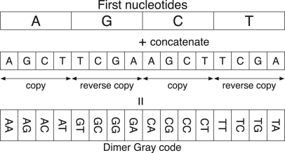
The DNA Gray code can be constructed iteratively from monomers to arbitrary length oligomers. Consider a monomer code (A,G,C,T). This code is obviously a Gray code because adjacent monomers differ by one nucleotide. Note that we regard the last monomer to be adjacent to the first monomer, and this circularity holds for longer oligomers. We prepare four copies of the monomer Gray code and concatenate them with each nucleotide, but in the cases of G and T, the copies are arranged in the reverse order. This procedure yields the dimer Gray code as illustrated in Figure 1. In the same manner as the dimers, we can construct the DNA Gray code of k-mers (k>1) by preparing four copies of the (k−1)-mer Gray code, two of which are reversed and concatenating them to each nucleotide.

Fig. 1.

Construction process of the DNA Gray code of dimers. The ordinary and reverse copies in the second row are copied from the monomer Gray code in the first row. The concatenation of the first and second rows yields the dimer Gray code shown in the third row.

In general, if the (k−1)-mer code is a Gray code, the k-mer code constructed by the above procedure is also a Gray code. This fact can be understood from the following observations. We can partition the k-mer Gray code into four regions in which the first nucleotides in each region are identical. Inside each region, the oligomers are arranged in Gray code order because the first nucleotides are identical and the others are the (k−1)-mer Gray code. On the other hand, two oligomers at both sides of a boundary between neighboring regions are identical except for the first nucleotides because of the reverse copy. Consequently, the k-mer code is inductively a Gray code as the monomer code is a Gray code.

The DNA Gray code has an ordered tree structure as a consequence of the construction process mentioned above (Er, 1984). This implies that we can apply the depth-first search algorithm to the tree to naturally order oligomers of variable lengths. This feature is important in combining the DNA Gray code with the equiprobable oligomers, as discussed later in Section 2.3.

The Hamming distance between oligomers located at a distance d in the DNA Gray code is smaller than or equal to d. In this regard, when we extract some consecutive oligomers from the DNA Gray code, those oligomers are similar to one another. However, all similar oligomers are not necessarily in a neighborhood in the DNA Gray code, i.e. two oligomers having a small Hamming distance can be located at distant positions. Nevertheless, we can show that the property of the neighboring similarity is beneficial for efficient data processing compared with conventional methods (Section 3).

2.2 Shift detection

Two oligomers with a shift relation, for example ACGGT and CGGTC, are similar to each other in the sense of edit distance, although the Hamming distance between them is large. Because of the large Hamming distance, we cannot immediately detect the similarity between such oligomers in the DNA Gray code. Fortunately, however, we can detect the shift relations of the oligomers at a low cost by taking advantage of the feature that the DNA Gray code is left shift continuous.

Let S be a semi-infinite sequence, S=s₀s₁···s_i···, s_i∈{A,G,C,T}. The left shift σ of the sequence is defined by:

(1)

Note that the left shift is the inverse of the construction of the DNA Gray code; in the construction process, we concatenate oligomers with each nucleotide, whereas we remove the first nucleotides from the oligomers in the left shift.

To explain the left shift continuity, we introduce a real-valued representation of the sequence in the DNA Gray code. Let G_k={g₀, g₁,…, g_i,…, g_N−1} be a DNA Gray code with N=4^k oligomers, where g_i is an oligomer of length k, g_i=s_i0s_i1···s_ik−1. The real-valued representation ϕ_k of g_i is defined by:

(2)

In general, there is also a real-valued representation ϕ of a semi-infinite sequence S, x=ϕ(S) as k→∞. Our aim here is to show the function f that corresponds to the left shift σ in the real-valued domain x.

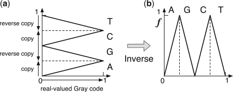
In order to understand the left shift function f, we consider the construction process of the DNA Gray code in the real-valued domain, as shown in Figure 2. The copies and reverse copies in the construction process correspond to the linear maps that have positive and negative slopes in the real-valued domain, respectively. Therefore, the process is expressed as shown in Figure 2a. Since the left shift is the inverse process of the construction, we can obtain the left shift function as the inverse map, as shown in Figure 2b. This function is equivalent to the composition map of the tent map well known in chaos theory (Alligood et al., 1997).

Fig. 2.

Construction process and left shift of the DNA Gray code in the real-valued domain. (a) The construction process can be expressed as linear maps that have positive (A and C) and negative (G and T) slopes. (b) The left shift function f can be understood as the inverse of the construction process.

It should be noted that the function f is continuous. The left shift continuity implies that the image mapped from a contiguous region in the DNA Gray code, which corresponds to a set of similar oligomers, is also contiguous. If the functions were discontinuous, a contiguous region would be mapped to scattered regions. The left shift continuity ensures that we can obtain a single region whenever a contiguous region is mapped.

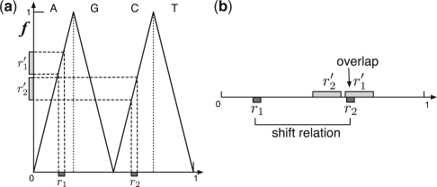
Figure 3 illustrates two examples of contiguous regions r₁ and r₂, and their images r^′₁ and r^′₂. The region r₂ overlaps with the image r^′₁ (Fig. 3b), which corresponds to the left shifts of oligomers in r₁ (Fig. 3a). Since this implies that r₂ is included in the left shifts of r₁, we can judge that those regions have a shift relation. Thanks to the left shift continuity, a shift relation can be detected by mapping only two oligomers at the beginning and end of the region even though the contiguous region is composed of many oligomers.

Fig. 3.

Mappings from two contiguous regions (r₁ and r₂) to their images (r^′₁ and r^′₂). (a) The relations between the contiguous regions and their images are indicated on the left shift function f. (b) All contiguous regions are illustrated on the same unit line. Since the region r₂ overlaps with the image r^′₁, there is a shift relation between r₁ and r₂.

To detect overlapped pairs in a set of contiguous regions, we compare the regions with a sorted list of their images. We can compare those lists in a linear order of the number of regions. Consequently, we can detect shift relations of oligomers quite efficiently.

2.3 Equiprobable oligomers

The background probability is a model that represents an intrinsic property of DNA sequences regardless of the presence of motifs. We can statistically detect an oligomer as a motif when the frequency of its occurrence is significantly higher than the background probability. In this work, we use the m-th order Markov model of the given sequences as the model of the background probability.

As we mentioned in Section 1, a variation among the background probabilities causes statistical bias in the significance detection. To overcome this problem, we propose equiprobable oligomers whose lengths are variable, but whose background probabilities are adjusted to be nearly identical to one another.

Let I(S) be the background information content of an oligomer S, where I(S)=−log₂ P(S) and P(S) is the background probability. Let S^′ be the oligomer in which the right-most nucleotide is removed from S. We define the equiprobable oligomer S such that it has the following property,

(3)

where θ is a threshold parameter.

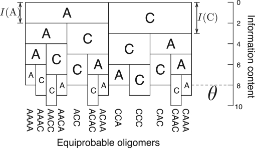
As an example, we consider equiprobable oligomers that consist of only A and C with the 0-th order Markov model as the background probability. In the 0-th order Markov model, the background information content I(S) of an oligomer S is expressed as the sum of the background information contents of individual nucleotides, i.e. I(S)=I(s₀s₁···s_k−1)=∑_i=0^k−1I(s_i). Figure 4 illustrates such equiprobable oligomers. Each box corresponds to a nucleotide and its height is drawn to be proportional to the information content of that nucleotide. Therefore, when the (downwardly) heaped boxes exceed the threshold θ, the column of those nucleotides becomes an equiprobable oligomer. All the equiprobable oligomers do not have exactly the same probability; for example, I(AAAA)=8 and I(CCC)=9. However, the equiprobability is considerably improved compared with fixed-length oligomers, especially in the cases of longer oligomers and a higher order Markov model. The validity of the digitizing approximation is discussed in Section S.1 in Supplementary Material.

Fig. 4.

An example of equiprobable oligomers arranged in the order of Gray code. We use the 0-th order Markov model with I(A)=2 and I(C)=3. We fix the threshold parameter θ=8. The height of a box corresponds to its information content.

Consider two oligomers, S₁ and S₂, such that S₁ is shorter than S₂. If S₂ is an equiprobable oligomer and S₁ matches a prefix of S₂, S₁ cannot be an equiprobable oligomer because I(S₁) should be smaller than θ under the property of Equation (3). This observation implies that the set of equiprobable oligomers is a prefix code in which no oligomer matches a prefix of any other oligomer. Recall the feature that the DNA Gray code has the ordered tree structure. In the prefix code, a code word is always located at a leaf of the tree. Therefore, the equiprobable oligomers can be ordered on the tree and hence we can naturally combine the equiprobable oligomers with the DNA Gray code so that adjacent oligomers differ from each other by just one nucleotide up to the length of the shorter oligomer.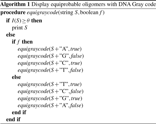

Algorithm 1 shows the recursive procedure that performs the depth-first search on the tree of the DNA Gray code. By calling equigraycode(″″,true), one can display all of the equiprobable oligomers with the DNA Gray code. If we use the i.i.d. uniform distribution as the background model, we can obtain the DNA Gray code with a fixed length of θ/2, because I(S)=2|S| in this case. Therefore, Algorithm 1 can generate the DNA Gray code as a special case.

2.4 Significance detection

We have now obtained the DNA Gray code of equiprobable oligomers. To detect significant motifs from a given set of sequences, we count the occurrences of equiprobable oligomers. Let C be a set of occurrence counts of equiprobable oligomers:

(4)

where M is the number of equiprobable oligomers and c_i is the count of the i-th oligomer in the DNA Gray code. We define a contiguous region [i, j] as a cluster if it satisfies the following conditions,

(5)

The cluster is a set of similar oligomers that appear in the given sequences.

We detect the significance of the cluster by using its width w=j−i+1 and the total count o=∑_k=i^j c_k. The null hypothesis is that the cluster is obtained from random sequences generated by the background model. In the background model, the occurrence probability p of each oligomer can be approximated by p=1/M because oligomers are equiprobable. Let q be the probability of an oligomer that occurs at least once. Thus, q is expressed as q=1−(1−p)^T, where T is the total number of oligomers in the given sequences. The random width W against w can be understood as Bernoulli trials where there are W-successes with the probability q between two failures. Therefore, the probability distribution of W is a geometric distribution represented by:

(6)

Since O≥w, the random total count O against o is conditioned by the width w. If there is no constraint, the probability distribution of O is a binomial distribution with the success probability wp and the number of observations T. The conditional probability distribution is represented by:

(7)

where Bin is the binomial distribution:

(8)

Using these distributions, we define the p-value pv of a cluster by:

(9)

Since there are many clusters in the set of occurrence counts C, a large number of significance tests must be involved. To reduce the false discovery rate, we use the e-value ev instead of the p-value, which is adjusted by the number of equiprobable oligomers M as follows,

(10)

If ev is smaller than a significance level α, the null hypothesis is rejected and hence the corresponding cluster is judged to be significantly enriched.

2.5 Summary of methods

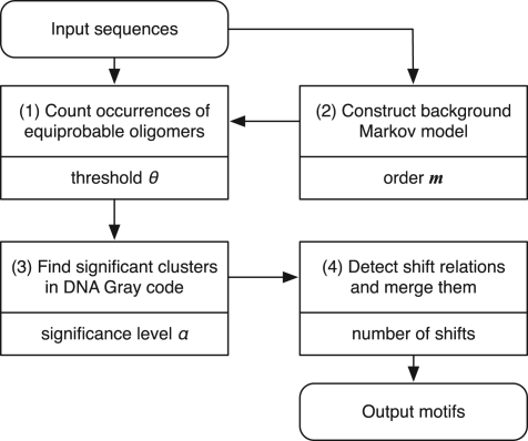
The flowchart shown in Figure 5 summarizes our motif discovery procedure. The parameter that characterizes each process is presented beneath the description of the process.

1. Threshold parameter θ: the threshold parameter θ is critical in our method because it regulates the probability of equiprobable oligomers p. Empirically, we can obtain good results when we set p=1/L, where L is the total sum of the lengths of the input sequences. Therefore, in the application, θ is automatically adjusted in accordance with the input sequences, such that θ=log₂(L)−ϵ (empirically, ϵ=1). The rationale behind this estimation is discussed in Section S.2 in Supplementary Material.

2. Order of Markov model m: the background Markov model is constructed from the input sequences that include the motifs themselves. Since the regions occupied by the motifs are much smaller than the rest of the sequences, the background model can be properly estimated if m is small. The default value of m is fixed at 3.

3. Significance level α: the significance level α is not crucially influential in our method. We set the default value at 0.01 as a typical value.

4. Number of shifts: after finding significant clusters, we sort them in the ascending order of their e-values. We pick up each cluster in this order and look for other clusters that have a shift relation with it. The clusters thus found are merged into a single motif. This process is recursively performed. The depth of this recursion defines the number of shifts allowed. We set the default value for the depth at 3.

Fig. 5.

Flowchart of the motif discovery. Each box that corresponds to a process presents the description (upper) and the parameter (lower) within it.

2.6 Data and statistics

As the benchmark data, we use the set of human promoter sequences in the cisRED database (Human v9.0, Robertson et al., 2006). The cisRED database consists of a set of promoter sequences and a set of motifs defined in those sequences, where each motif is conserved among several species and annotated according to the known motif database TRANSFAC (Wingender, 2004). The number of promoter sequences is 18 779. The total number of nucleotides is ~47 Mbp, of which valid (unmasked) nucleotides amount to ~31 Mbp. After removal of redundancy, the number of conserved motifs is 236 208 and the number of nucleotides occupied by the motifs is ~2.3 Mbp.

By comparing the sites predicted by our method with those listed in the cisRED database, we assess the performance of our method at two distinct levels, the nucleotide level and the site level. The statistics we use are essentially the same as those adopted by Tompa et al. in their assessment strategy (Tompa et al., 2005). At the nucleotide level, each dataset consists of pairs (i,p), where i is the sequence ID and p is the nucleotide position within the site. We denote the sets of known sites and predicted sites by nK and nP, respectively. At the site level, each set consists of triples (i,s,e), where i is the sequence ID, and s and e are the start and end positions of the site, respectively. We denote the sets of known and predicted sites by sK and sP, respectively.

At the nucleotide level, the true positive nTP is simply defined by:

(11)

where |·| implies the size of the set. At the site level, the true positive sTP is expressed as:

(12)

where ov(u, v)=min(u.e,v.e)−max(u.s,v.s)+1 (overlap) and len(u)=u.e−u.s+1 (length). This expression implies that sTP is the number of known sites that overlap with the predicted sites by at least one-quarter of the length of the known site.

The false positive and the false negative are defined as follows,

(13)

where x=n (nucleotide level) or x=s (site level). The true negative is defined only at the nucleotide level:

(14)

where L is the number of valid nucleotides in the promoter sequences.

Of the above definitions, only the false positive at the site level sFP is different from that of Tompa et al. (2005). Tompa et al. allowed overlaps between the predicted sites and removed such sites from sFP if each site overlapped with a known site. In contrast, we use a slightly more stringent criterion to check whether the clustering of motifs is appropriately performed, i.e. we include the overlaps of the predicted sites in sFP even if the sites overlap with a known site.

Either at the nucleotide (x=n) or at the site (x=s) level, the sensitivity xSn and the positive predictive value xPPV are defined as usual:

(15)

and

(16)

To average these quantities to give a single statistic, we adopt the correlation coefficient nCC at the nucleotide level, which is defined by:

(17)

In a similar way, we adopt the average site performance sASP at the site level, which is defined by:

(18)

3 RESULTS AND DISCUSSION

3.1 Performance evaluation with all motifs in cisRED

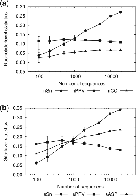
To examine the performance of our method, Hegma, we adopt essentially the same evaluation scheme as that used by Tompa et al. (2005). To evaluate the effects of data size on the performance, we prepare sets of sequences that are randomly selected from the human promoter sequences of the cisRED database. In the following results shown in Figure 6, we prepare 10 sets for each number of sequences.

Fig. 6.

Prediction statistics at the nucleotide level (a) and the site level (b), as a function of the number of sequences. The default parameter set described in Section 2.5 is used for calculation. Each symbol indicates the average of 10 tests with the sequences randomly selected from the full data. Error bars indicate the maximum and minimum values of the statistics. The right-most statistics correspond to those for the full data: where nSn=0.27, nPPV=0.11 and nCC=0.067 at the nucleotide level; sSn=0.34, sPPV=0.13 and sASP=0.23 at the site level.

Figure 6a indicates that nPPV at the nucleotide level is insensitive to the variation in the number of sequences. In the default setting, our method adjusts the threshold parameter such that the equiprobable oligomers should have the probability p=1/L under the background model, as discussed in Section 2.5. This adjustment maintains the null distribution at a constant precision, which accounts for the constant rate of false positive (or type I error) and hence nearly constant nPPV. In contrast, nSn is improved as the number of sequences is increased. This improvement can be explained by the general characteristics of statistical analysis, where a larger data size leads to more precise results.

The results at the site level are similar to those at the nucleotide level except that sPPV decreases for larger numbers of sequences (Fig. 6b). This decrease in sPPV originates from overlaps between predicted sites, which augment sFP under our definition. Our method can detect a shift relation between overlapped sites and merge them. If this process were perfectly performed, the overlaps of the predicted sites would be repressed. However, we fail to eliminate all the overlaps partly because we restrict the size of shifts to 3 in the default setting. We impose this restriction to avoid the risk of merging unrelated motifs. Improved discrimination between related and unrelated motifs is one task to be explored in the future.

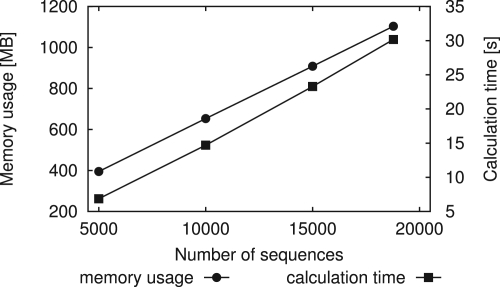
Figure 7 shows the memory usage and the calculation time. Calculations are made on a computer with 3 GHz Intel Xeon^® with 16 GB memory running under Linux^® 2.6. Both time and memory linearly increase with the number of sequences. It is noteworthy that we need only 30 s for calculation of the full data (18 779 sequences, 31 Mb). The memory usage of 1.1 GB is also sufficiently feasible for current conventional computers.

Fig. 7.

Dependence of memory usage and calculation time on the number of sequences. Each value is the average of 10 trials. For the full data, the memory usage is 1.1 GB and the calculation time is 30 s.

3.2 Performance evaluation with specific motifs

We compare the performance of our method to that of Weeder (version 1.4.2, Pavesi et al., 2004), a representative word-based method based on exhaustive enumeration with a limited number of mutations. We choose Weeder because it performed best in the assessment of Tompa et al. (2005).

Almost all the conventional tools, including Weeder, assume that given promoter sequences are derived from coregulated genes. This assumption implies that most of the given sequences have at least one specific motif that contributes to the specific regulation. Therefore, we prepare a set of sequences in which the fraction of sequences holding the motif is variably specified. We adopt the motif AhR as the specific motif, because it is the most frequent motif in the TRANSFAC annotations. Let R and U be the sets of sequences with and without the motif AhR, respectively. We select sequences from R and U according to a predefined percentage that we control. For example, when the total number of sequences is 1000 and the percentage of motif-containing sequences is 80%, we select 800 sequences from R and 200 sequences from U. In the following results, we fix the number of sequences at 1000. In order to evaluate the performance of single-motif detection, we regard only the known sites as the right sites of the motif AhR, even though the motifs may be present at other sites in the sequence.

We run Weeder under the following settings: the species code is HS; the minimal sequence percentage on which the motif has to appear is 5 (to increase sensitivity); and the top 20 000 (sufficiently large) motifs are reported. We try the following pairs of motif length and maximal number of mutations: (6,1), (8,2) and (10,3). Although motif length 12 is also allowed, we do not try it because of the prohibitively long calculation time. We determine the positions of the predicted sites with the tool locator.out included in the Weeder tools.

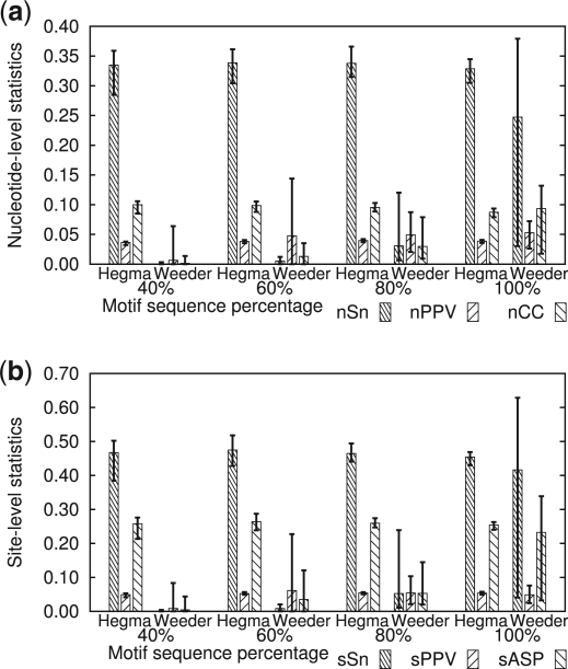
Figure 8a shows the results at the nucleotide level. When the percentage of motif-containing sequences is 100%, i.e. all the sequences have the specific motif AhR, nCC of Weeder (0.093) is superior to that of Hegma (0.087). However, Hegma outperforms Weeder under all other situations. The performance of Weeder becomes worse as the percentage of motif-containing sequences decreases, whereas Hegma is little affected by this variation. Since the average length of equiprobable oligomers in this evaluation is 10.7, our setting of the motif length of Weeder should be impartial. Furthermore, Weeder also adopts statistical measures based on Z-score, in a similar way to our method. Therefore, it is most likely that the equiprobable oligomers adopted in Hegma contribute to improving performance compared with the fixed-length oligomers used in Weeder.

Fig. 8.

Performance comparison between Hegma and Weeder at the nucleotide level (a) and the site level (b). The number of sequences is fixed at 1000. Boxes show the average values of statistics of 10 sets of sequences. Error bars show the maximum and minimum values of statistics. The fractions of the motif-containing sequences are varied from 40% to 100%. The parameter setting of our method is default. See the text for the parameter setting of Weeder.

The results at the site level (Fig. 8b) are more remarkable than those at the nucleotide level. At this level, Hegma outperforms Weeder under all situations, including the case that 100% of the sequences contain the motif, where sASP of Weeder is 0.23 and that of Hegma is 0.25. We consider that the merge of shift-related motifs introduced in Hegma has effectively reduced sFP and hence improved sPPV, as mentioned in the previous subsection.

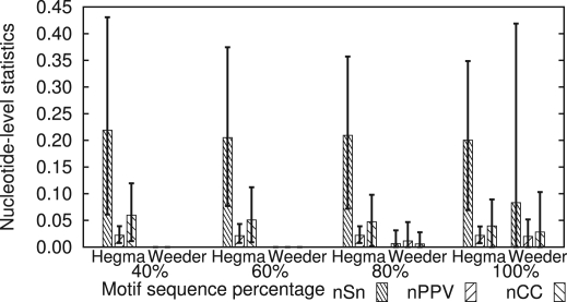
We repeat the same analysis as mentioned above for the 10 most frequent motifs in cisRED (AhR, aMEF-2, POU2F1, Pax-5, DEAF-1, CREB, HNF-1α, DP-1, RSRFC4 and POU3F2). Figure 9 summarizes the results for these 10 motifs at the nucleotide level by averaging their statistics. The detailed results for individual motifs together with the results of non-parametric statistical tests are presented in Section S.4 in Supplementary Material. Clearly, Hegma outperforms Weeder under all the situations tested. The results at the site level are also similar to those at the nucleotide level (data not shown). These observations imply that the performance of Hegma is more stable than that of Weeder regardless of the type of motif as well as the fraction of sequences that contain the motif. An additional examination on a smaller ChIP-seq peak dataset also supports this conclusion as shown in Section S.3 in Supplementary Material.

Fig. 9.

Average statistics for the 10 most frequent motifs at the nucleotide level. Boxes show the average values for the statistics of motifs. Error bars show the maximum and minimum values of the statistics. The setting is the same as that in Figure 8.

The average calculation time per dataset (1000 sequences) for Weeder is 10 h, whereas that for our method is only 1.4 s when tested under the same condition mentioned in Section 3.1 and averaged over 40 trials. Therefore, our method shows considerable advantage in calculation time as well.

3.3 Analysis of unannotated motifs

In Section 3.1, we regard the predicted sites that do not match any cisRED annotation as ‘false positives’. However, it is probable that some of them actually represent true motifs absent from the cisRED annotation. We then extract such unannotated motifs from all significant motifs predicted by Hegma in the full data of the cisRED promoters such that >95% of the sites comprising each motif do not overlap with any annotated sites. The number of all the predicted motifs is 7528 (composed of a total of 620 153 sites), of which the number of unannotated motifs is 1161 (36 443 sites). Figure 10 illustrates four examples of the unannotated motifs with the smallest e-values in sequence logos (Schneider and Stephens, 1990).

Fig. 10.

Four examples of unannotated motifs absent from the cisRED annotation. Each motif is labeled according to the name of the most similar motif in the JASPAR database (Sandelin et al., 2004). We selected these motifs as the ones with the smallest e-values: (1) ev = 6.2×10⁻⁶⁴, (2) 1.2×10⁻⁴⁰, (3) 1.9×10⁻³⁵ and (4) 8.6×10⁻³⁵.

The unannotated sites tend to be located in distal regions compared with all the predicted sites; the average position (±SD) of the unannotated sites is −1140±894 bp relative to the transcription start sites, whereas that of all the predicted sites is −737±837 bp (p-value of t-test: ≈0). The unannotated sites are a subset of the predicted sites and its complementary set is associated with the cisRED annotation. Therefore, this disparity suggests that the positions of the annotated sites in cisRED may have significant bias toward proximal regions. These observations may be interpreted as follows; it may be difficult for a phylogenetic footprinting approach, including cisRED, to detect conserved motifs in the distal regions, where the marked sequence divergence or the existence of repetitive elements hinders reliable sequence alignment compared with more conserved proximal regions (Suzuki et al., 2004). Therefore, our method can complement the phylogenetic footprinting approach to improve the overall sensitivity of motif discovery.

4 CONCLUSION

We have developed a large-scale motif discovery tool, Hegma, and shown that Hegma is not only applicable to large-scale data, but also can stably detect motifs even if only a small fraction of the examined sequences contain the motifs. Thus, Hegma is applicable to situations where the fraction of motif-containing sequences is uncontrollable, such as the detection of splicing enhancers or silencers in exon and intron sequences, or the detection of microRNA binding sites in UTR sequences. A huge number of such sequences have already been collected in databases. However, as our knowledge of those motifs is yet far from complete, it is difficult to know in advance the percentage of sequences holding the motifs. We consider that the speed and precision of Hegma would facilitate discovery of novel motifs from a heap of sequence data.

Funding: Aihara Innovative Mathematical Modelling Project, Japan Society for the Promotion of Science (JSPS) through the ‘Funding Program for World-Leading Innovative R&D on Science and Technology (FIRST Program)’, initiated by the Council for Science and Technology Policy (CSTP); Grants-in-Aid (No. 20651053, No. 221S0002 and No. 22310124) from the Ministry of Education, Culture, Sports, Science and Technology of Japan, in part.

Conflict of Interest: none declared.

REFERENCES

- Alligood K.T., et al. Chaos. an Introduction to Dynamical Systems. New York, LLC: Verlag; 1997. [Google Scholar]
- Bailey T.L., Elkan C. Proceedings of the 2nd International Conference on Intelligent Systems for Molecular Biology. Menlo Park, California: AAAI Press; 1994. Fitting a mixture model by expectation maximization to discover motifs in biopolymers; pp. 28–36. [PubMed] [Google Scholar]
- Das M., Dai H.-K. A survey of DNA motif finding algorithms. BMC Bioinformatics. 2007;8(Suppl. 7):S21. doi: 10.1186/1471-2105-8-S7-S21. [DOI] [PMC free article] [PubMed] [Google Scholar]
- Er M.C. On generating the N-ary reflected gray codes. IEEE Trans. Comp. 1984;C-33:739–741. [Google Scholar]
- Gray F. Pulse code communication. U.S. Patent 2632058. 1947 [Google Scholar]
- Lawrence C.E., et al. Detecting subtle sequence signals: a Gibbs sampling strategy for multiple alignment. Science. 1993;262:208–214. doi: 10.1126/science.8211139. [DOI] [PubMed] [Google Scholar]
- Pavesi G., et al. Weeder Web: discovery of transcription factor binding sites in a set of sequences from co-regulated genes. Nucleic Acids Res. 2004;32:W199–W203. doi: 10.1093/nar/gkh465. [DOI] [PMC free article] [PubMed] [Google Scholar]
- Robertson A.G., et al. cisRED: a database system for genome scale computational discovery of regulatory elements. Nucleic Acids Res. 2006;34:D68–D73. doi: 10.1093/nar/gkj075. [DOI] [PMC free article] [PubMed] [Google Scholar]
- Sandelin A., et al. JASPAR: an open-access database for eukaryotic transcription factor binding profiles. Nucleic Acids Res. 2004;32(Suppl. 1):D91–D94. doi: 10.1093/nar/gkh012. [DOI] [PMC free article] [PubMed] [Google Scholar]
- Sandve G.K., Drabløs F. A survey of motif discovery methods in an integrated framework. Biol. Direct. 2006;1:11. doi: 10.1186/1745-6150-1-11. [DOI] [PMC free article] [PubMed] [Google Scholar]
- Schneider T.D., Stephens R.M. Sequence logos: a new way to display consensus sequences. Nucleic Acids Res. 1990;18:6097–6110. doi: 10.1093/nar/18.20.6097. [DOI] [PMC free article] [PubMed] [Google Scholar]
- Suzuki Y., et al. Sequence comparison of human and mouse genes reveals a homologous block structure in the promoter regions. Genome Res. 2004;14:1711–1718. doi: 10.1101/gr.2435604. [DOI] [PMC free article] [PubMed] [Google Scholar]
- Tompa M., et al. Assessing computational tools for the discovery of transcription factor binding sites. Nat. Biotechnol. 2005;23:137–144. doi: 10.1038/nbt1053. [DOI] [PubMed] [Google Scholar]
- Wakaguri H., et al. DBTSS: database of transcription start sites, progress report 2008. Nucleic Acids Res. 2008;36(Suppl. 1):D97–D101. doi: 10.1093/nar/gkm901. [DOI] [PMC free article] [PubMed] [Google Scholar]
- Wingender E. TRANSFAC, TRANSPATH and CYTOMER as starting points for an ontology of regulatory networks. In Silico Biol. 2004;4:55–61. [PubMed] [Google Scholar]
Associated Data
This section collects any data citations, data availability statements, or supplementary materials included in this article.