Abstract
Microarray analysis promises to detect variations in gene expressions, and changes in the transcription rates of an entire genome in vivo. Microarray gene expression profiles indicate the relative abundance of mRNA corresponding to the genes. The selection of relevant genes from microarray data poses a formidable challenge to researchers due to the high-dimensionality of features, multiclass categories being involved, and the usually small sample size. A classification process is often employed which decreases the dimensionality of the microarray data. In order to correctly analyze microarray data, the goal is to find an optimal subset of features (genes) which adequately represents the original set of features. A hybrid method of binary particle swarm optimization (BPSO) and a combat genetic algorithm (CGA) is to perform the microarray data selection. The K-nearest neighbor (K-NN) method with leave-one-out cross-validation (LOOCV) served as a classifier. The proposed BPSO-CGA approach is compared to ten microarray data sets from the literature. The experimental results indicate that the proposed method not only effectively reduce the number of genes expression level, but also achieves a low classification error rate.
Key words: feature selection, genetic algorithm, K-nearest neighbor, microarray, particle swarm optimization.
1. Introduction
Microarray analysis promises to detect variations in gene expressions, and changes in the transcription rates of an entire genome in vivo. A microarray chip manufactured by high-speed robotics, enables researchers to simultaneously put thousands of samples on a glass slide. The principle behind the microarray is the placement of specific nucleotides sequence in an orderly array, which then will be hybridized by fluorescent DNA or RNA markers. The location and intensity of the fluorescent spot on the glass slide reveals the extent of the transcription of a particular gene. Microarrays are not limited to nucleic acid analysis. Protein microarrays and tissue microarrays were originally introduced to study protein-drug interaction, and the relationship between individual genes and diseases. They have subsequently been applied successfully to the treatment of patients. Experimental data from microarrays is routinely gathered, and the amount of information contained in microarray data is becoming enormous. This abundance of information necessitates very complex biostatistical methods, many of which are still under development, to correctly interpret the information available (Forozan et al., 2000).
Discriminant analysis of microarray data has great potential as a medical diagnosis tool, since results represent the state of a cell at the molecular level. Microarray data is used in medical applications since it is possible to analyze gene expression characteristics and forecast the treatment of human diseases (Chang et al., 2005; Jeffrey et al., 2005; Lonning et al., 2005). Microarray data contains a large number of features with high-dimensions, consists of multiclass categories, and is usually of a small sample size, all of which makes testing and training of general classification methods difficult. With the rapid increase of computational power for data analysis suitable algorithms have become a very important issue. A suitable algorithm selects any optimum subset of genes that may be representing a disease gene combination.
The classification of gene expression data samples involves feature selection and classifier design. A reliable selection method for genes relevant for sample classification is needed in order to increase classification accuracies and to avoid incomprehensibility. Feature selection is the process of choosing a subset of features from the original feature set; it can thus be viewed as a principal pre-processing tool when solving classification problems (Choudhary et al., 2006; Wang et al., 2007). Theoretically, feature selection problems are NP-hard. It is impossible to conduct an exhaustive search over the entire solution space since this would take a prohibitive amount of computing time and cost (Cover and Van Campenhout 1977). The goal is to select a subset of d features (genes) from a set of D features (d < D) in a given gene expression data set (Oh et al., 2004). D is comprised of all features (genes) in a gene expression data set and may include noisy, redundant and misleading features. We therefore aimed to delete irrelevant features and only kept features relevant for classification. Deleting irrelevant features improves the computational efficiency. Furthermore, decreasing the number of features results in a reduced classification error rate. An increasing number of evolutionary and optimization algorithms (Deutsch, 2003) have been applied to feature selection problems, such as genetic algorithms (GAs) (Oh et al., 2004), particle swarm optimization (PSO) (Wang et al., 2007), and tabu search (TS) (Tahir et al., 2007).
Identifying an optimal subset of features, i.e., relevant genes, is a very complex task in bioinformatics (Hua et al., 2005). Successful identification usually focuses on the determination of a minimal number of relevant genes combined with a decrease of the classification error rate (Huang and Chang, 2007). Statistical methods applied to microarray data analysis include the linear discriminant analysis (Dudoit et al., 2002; Lee et al., 2005; Li et al., 2004), the K-nearest neighbor method (Cover and Hart, 1967), support vector machines (Furey et al., 2000; Huang and Chang, 2007; Lee and Lee, 2003; Ramaswamy et al., 2001), Random Forest (RF) (Diaz-Uriarte and de Andres, 2006), instance-based methods (Berrar et al., 2006), entropy-based methods (Liu et al., 2005), and shrunken centroids (Tibshirani et al., 2002).
In general, two crucial factors to determine the performance of gene expression classification problem can be identified; these are gene feature selection and classifier design. Hence, in addition to the selected relevant gene subsets, the classification results also depend on the performance of the classifiers. The challenge in classifier design is to extract the proper information from the training samples and to allocate the samples contained in the previously defined diagnostic classes by measurements of expression of the selected genes (Buturovic, 2006). Choosing the correct category of the selected genes is a complicated assignment. In classifier design, solving a multi-class (class >2) classification problem is generally more difficult than solving a classification problem with only two-classes. The K-nearest neighbor (K-NN) method (Deutsch, 2003; Zhu et al., 2007) and support vector machines (SVMs) (Furey et al., 2000; Huang and Chang, 2007) are two prevalent classifiers for gene classification problems. In our study, we adopted the K-nearest neighbor method. The K-nearest neighbor procedure works based on a minimum distance from the testing sample to the training samples to determine the K nearest neighbors. For error estimation methods on the classifier, a widely used approach is cross-validation (CV). The leave-one-out cross-validation (LOOCV) procedure is a straightforward technique and gives an almost unbiased estimator (Jirapech-Umpai and Aitken, 2005). LOOCV can be used in small sample-sized data sets. The functionality of the classifier for the error estimation is thus reduced for multi-class categories and small sample sizes of the gene microarray data.
Evolutionary algorithms with their heuristics and stochastic properties often suffer from getting stuck in local optimum. These common characteristics led to the development of evolutionary computation as an increasingly important field. A GA is a stochastic search procedure based on the mechanics of natural selection, genetics and evolution. Since this type of algorithm simultaneously evaluates many points in the search space, it is more likely to find a global solution to a given problem. PSO describes a solution process in which each particle flies through the multidimensional search space. The particle velocity and position are constantly updated according to the best previous performance of the particle or of the particle's neighbors, as well as the best performance of the particles in the entire population. Hybridization of evolutionary algorithms with local search has been investigated in many studies (Kao and Zahara, 2008; Lovbjerg et al., 2001). Such a hybrid is often referred to as a memetic algorithm. Memetic algorithms can be treated as a genetic algorithm coupled with a local search procedure (Sorensen and Sevaux, 2006). In this article, instead of using a memetic algorithm, we combined two global optimization algorithms, i.e., a combat genetic algorithm (CGA) and binary particle swarm optimization (BPSO). We employed the hybrid BPSO-CGA algorithm to implement feature selection. The CGA is embedded in the BPSO and performs the role of a local optimizer for each generation. The K-nearest neighbor method (K-NN) with leave-one-out cross-validation (LOOCV) based on Euclidean distance calculations served as a classifier of the BPSO and CGA on ten microarray data sets taken from the literature (Diaz-Uriarte and de Andres, 2006).
In order to evaluate the performance of BPSO-CGA, we compared our experimental classification result with other results reported in the literature (Diaz-Uriarte and de Andres, 2006). These literature methods consisted of four distinct methods, namely two versions of RFs (s.e. = 0 and s.e. = 1), nearest neighbor with variable selection (NN.vs), and shrunken centroids (SC.s). In addition to these methods from the literature, we also compared our proposed BPSO-CGA with pure BPSO. Experimental results show that BPSO-CGA not only reduce the number of features, but also prevented the BPSO procedure from getting trapped in a local optimum and thereby lowering the classification error rate.
2. Methods
2.1. Binary particle swarm optimization
Particle Swarm Optimization (PSO) is one of several population-based evolutionary computation techniques developed in 1995 by Kennedy and Eberhart (1995). PSO simulates the social behavior of birds and fish. This behavior can be described as a swarm intelligence system. In PSO, each solution can be considered a particle in a search space, with an individual position and velocity. During movement, each particle adjusts its position by changing its velocity based on its historical experience and the best experience of its neighboring particles, until it reaches an optimum position (Kennedy, 2006). All of the particles have fitness values based on the calculations of a fitness function. Particles are updated by following two parameters called pbest and gbest at each iteration. Each particle is associated with the best solution (fitness) the particle has achieved so far in the search space. This fitness value is stored, and represents the position called pbest. The value gbest is a global optimum value for the whole population.
PSO was originally developed to solve real-value optimization problems. Many optimization problems occur in a space featuring discrete, qualitative distinctions between variables and levels of variables. To extend the real-value version of PSO to a binary/discrete space, Kennedy and Eberhart (1997) proposed a binary PSO (BPSO) method. In a binary search space, a particle may move to near corners of a hypercube by flipping various numbers of bits; thus, the overall particle velocity may be described by the number of bits changed per iteration (Kennedy and Eberhart, 1997).
The position of each particle is represented by Xp = {Xp1, Xp2, …, Xpd} and the velocity of each particle is represented by Vp = {Vp1, Vp2, …, Vpd} (d is number of particles). In BPSO, once the adaptive values pbest and gbest are obtained, the features of the pbest and gbest particles can be tracked with regard to their position and velocity. Each particle is updated according to the following equations (Kennedy and Eberhart, 1997):
 |
(1) |
 |
(2) |
 |
(3) |
 |
(4) |
In Eq. 2, w is the inertia weight, c1 and c2 are acceleration parameters, whereas rand, rand1, and rand2 are three independent random numbers between [0, 1]. Velocities  and
and  are those of the updated particle and the particle before being updated, respectively,
  is the original particle position (solution), and
  is the updated particle position (solution). In Eq. 3, particle velocities of each dimension are tried to a maximum velocity
  . If the sum of accelerations causes the velocity of that dimension to exceed
  , then the velocity of that dimension is limited to
  .
.  and
and  are user-specified parameters (in our case
  ,
,  ). The updated features are calculated by the function
  (Eq. 4), in which
  is the updated velocity value. In Eq. 5, if
  is larger than a randomly produced disorder number that is within {0.0∼1.0}, then its position value
  is represented as {1} (meaning this feature is selected as a required feature for the next update). If
  is smaller than a randomly produced disorder number that is within {0.0∼1.0}, then its position value
  is represented as {0} (meaning this feature is not selected as a required feature for the next update).
2.2. Combat genetic algorithm
Genetic Algorithms (GAs) were developed by John Holland in 1975 (Holland, 1992). The concept is based on Darwin's theory of evolution and the survival of the fittest competition principles of natural selection. Based on evolutionary theory, the main principle of GAs is to randomly generate a population. GAs contain three evolutionary mechanism operators, namely selection, crossover, and mutation. After the three operators are applied, a new generation of the population will be generated. GAs randomly generate a set of chromosomes (solutions) at the same time. The chromosomes with a higher fitness value will be kept and calculated until a fixed number of iterations is reached, and then a final optimal fitness solution is output. GAs may fail to converge at a global optimum point depending upon the selective capacity of the fitness function (large variation of the fitness function for small variation of its input variables). Combat genetic algorithms (CGA), proposed by Eksin and Erol (Eksin and Erol, 2001; Erol and Eksin, 2006), are used to improve on the classic GA shortcoming of premature convergence by focusing on the reproduction aspect of a typical GA. Reproduction is one of the three major mechanisms in a GA that shift the chromosomes towards a local/global optimum point; it usually decreases the diversity of chromosomes though, which can be viewed as a source of premature convergence towards a local optimum point (Erol and Eksin, 2006). The CGA algorithms can be summarized as follows (Erol and Eksin, 2006):
Step1 Randomly generate initial population for m chromosomes.
Step2 Randomly select two distinct chromosomes from the population.
Step3 Evaluate the fitness value of the two selected chromosomes.
Step4 Calculate the relative difference value called r by using
 |
(5) |
where f1 and f2 are the fitness values of chromosome 1 and chromosome 2, respectively.
Step5 In compliance with the relative difference values, if the difference value is large, the partial overwrite operator is adopted, whereas if the difference value is small, the classic uniform crossover operation is chosen. This scenario can be divided into four cases:
(1) If f1 < f2 and R < r, crossover operation is assumed on the chromosome 2 and leave chromosome 1 unchanged, where R is a random number selected between [0, 1].
(2) If f1 < f2 and R > r, normal crossover operation is chosen.
(3) If f1 > f2 and R < r, crossover operation is assumed on chromosome 1 and chromosome 2 is left unchanged
(4) If f1 > f2 and R > r, normal crossover operation is chosen.
Step6 Mutation operation is set to a probability of 1/m. (m = number of chromosomes)
Step7 Stopping criteria is verified. If satisfied, the final solution is put out. Otherwise go to Step2.
2.3. K-nearest neighbor
The K-nearest neighbor (K-NN) method, one of the most popular nonparametric methods (Cover and Hart, 1967; Fix and Hodges, 1989; Hastie et al., 2005), is a supervised learning algorithm introduced by Fix and Hodges in 1951. K-NN classifiers have attracted the interest of many researchers due to their theoretic simplicity and the comparatively high accuracy that can be achieved with it compared other for complex methods (AltIncay, 2007). K-NN classifies objects which are represented as points defined in some feature space. The K-NN method is easy to implement since only the parameter K (number of nearest neighbors) needs to be determined. The parameter K is the most important factor affecting the performance of the classification process. In a multidimensional feature space, the data is divided into testing and training samples. K-NN classifies a new object based on the minimum distance from the testing samples to the training samples. The Euclidean distance was used in this article. If an object is near to a number of K nearest neighbors, it is classified into the K-object category. In order to increase the classification accuracy, the parameter K has to be adjusted according to the different data set characteristics.
In K-NN, a big category tends to have high classification accuracy, while the other minority classes tend to have low classification accuracy (Tan, 2006). In this article, the leave-one-out cross-validation (LOOCV) method was implemented on the microarray data classification. When there are n data to be classified, the data is divided into one testing sample and n-1 training samples at each generation of the evaluation process. The classifier is then constructed by training the n-1 training samples. The category of the test sample can be determined by the classifier. We set the parameter K to 1 directly, meaning that 1-NN with LOOCV was used as a classifier to calculate the classification error rates in our study.
2.4. Hybrid BPSO-CGA procedure
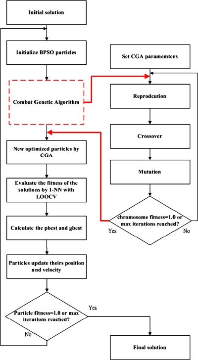
The hybrid BPSO-CGA procedure used in this study combined a BPSO and CGA for feature selection. The CGA was embedded within the BPSO and served as a local optimizer to improve the BPSO performance at each iteration. The flowchart of BPSO-CGA is shown in Figure 1. Initially, the position of each particle was represented by a binary (0/1) string  . D is the dimension of the microarray data; 1 represents a selected feature, while 0 represents a non- selected feature. For example, if D = 10, we obtain a random binary string S = 1000100010, in which only features F1, F5 and F9 are selected. The classification error rate of a 1-nearest neighbor (1-NN) was determined by the leave-one-out cross-validation (LOOCV) method that was used to measure the fitness of chromosomes and each particle. The BPSO-CGA procedure is described below:
FIG. 1.
Flowchart of the hybrid BPSO-CG.
Step1 Randomly generate an initial population for BPSO.
Step2 CGA is applied to generated particles, for reproduction, crossover and mutation.
Step3 Evaluate fitness values of all particles.
Step4 Check stopping criteria. If satisfied, go to Step 5. Otherwise go to Step 3.
Step5 Calculate the pbest and gbest values. Each particle updates its position and velocity via the BPSO update Eqs. (1) (2) (3) (4).
Step6 Check stopping criteria. If satisfied, output the final solution. Otherwise go to Step2.
The BPSO was configured to contain 20 particles and run for 100 iterations in each trial, or until a stopping criterion was met. The number of particles in the BPSO was equal to the number m of chromosomes in CGA (m = 20). After each generation of the BPSO, the CGA was run 30 times, for a total of 100 generations. The CGA parameters were taken from Erol and Eksin (Erol and Eksin, 2006). The classical uniform crossover operation applied in the CGA method is of the type proposed in the original CGA literature (Erol and Eksin, 2006). The mutation rate was also chosen based on the original literature. A mutation operator with a probability of 1/m (1/m = 1/20 = 0.05), with m being the population size, was used. We adopted the BPSO parameter values of Shi and Eberhart (1998). These values are claimed to be optimized. The acceleration factors c1 and c2 were both set to 2. The inertia weight w was 0.9.
3. Results
Due to the peculiar characteristics of microarray data (high number of genes and small sample size), many researchers are currently studying how to select relevant genes effectively before using a classification method to decrease classification error rates. In general, gene selection is based on two aspects: one is to obtain a set of genes that have similar functions and a close relationship; the other is to determine the smallest set of genes that can provide meaningful diagnostic information for disease prediction without trading off accuracy. Feature selection uses relatively fewer features since only selective features need to be used and will not affect the classification error rate in a negative way; on the contrary, classification error rate can even be decreased.
To compare the performance of the proposed BPSO-CGA, the experimental results obtained from the proposed method and the pure BPSO methods are compared with other results reported in the literature (Diaz-Uriarte and de Andres, 2006).
3.1. Microarray data sets
The microarray data sets were downloaded from http://ligarto.org/rdiaz/Papers/rfVS/randomForestVarSel.html (Diaz-Uriarte and de Andres, 2006). They consist of ten microarray data sets for Leukemia, Breast 2 class, Breast 3 class, NCI 60, Adenocarcinoma, Brain, Colon, Lymphoma, Prostate, and Srbct. First, the expression levels for each gene were normalized to [0, 1]. Normalizing the data is important to ensure that the distance measure allocates equal weight to each variable. Without normalization, the variable with the largest scale will dominate the measure (Tahir et al., 2005). The normalization procedure is given by equation (5). Valuemax is the maximum original value. Valuemin is the minimum original value. Valuemax is set to 1 and Valuemin is set to 0.
 |
(1) |
3.2. Exciting methods
In this study, we compared our experimental results to four distinct methods, namely two versions of RFs (s.e. = 0 and s.e. = 1), nearest neighbor with variable selection (NN.vs) and shrunken centroids (SC.s) developed by Diaz-Uriarte and Alvarez de Andres (2006).
RFs are classification methods based on decision trees. RFs consist of a large set of independent decision trees. The classification results depend on these decision tree classifications. The main reasons why RFs perform better than single decision trees is their ability to utilize irrelevant features and the independence of the different classifiers (trees) used (Sberveglieri, 2008). In RF, each tree is constructed using a different bootstrap sample of the data. Each node is split based on randomly chosen feature subsets. For the RF (s.e. = 0 and s.e. = 1) method developed by Diaz-Uriarte and Alvarez de Andres (2006), new forests are built iteratively at each iteration by deleting the genes with the largest out-of-bag (OOB) error and setting up the final set of genes. The OOB error rates from the fittings of all forests were scrutinized. Then u standard errors of the minimum error rate of all forests were used, with the bootstrap as a predictor. For u = 0, the subset of genes with the smallest error rate was selected. For u = 1, 1 s.e. rule from the literature (Breiman, 1984; Ripley, 2008), the solution was picked from all possible solutions with fewer genes and the same error rate.
Shrunken centroids (SC) are yet another kind of prediction method. In this method, standardized centroids are computed for each class. Then a threshold is used to shrink each of the class centroids toward the centroid of all classes (Sberveglieri, 2008). The threshold value is the only hyperparameter of SC. The optimal threshold is determined by cross-validation for a range of threshold values and then used to select the best feature subset. Usually, a number of genes that minimizes the cross-validated error rate are chosen. If there exist several solutions with the same minimal error rate, the one with the smallest number of genes is selected (Diaz-Uriarte and de Andres, 2006). Diaz-Uriarte and Alvarez de Andres (2006) used the 200 genes with the largest F-ratio from the literature results (Dudoit et al., 2002) and then chose the minimal cross-validated error rates with the smallest number of genes. Nearest Neighbor with variable selection (NN.vs) means that all genes are first ranked based on their F-ratio, and then a Nearest Neighbor classifier (KNN with K = 1) is calculated for all features subsets that result from eliminating 20% of the genes (the ones with the smallest F-ratio) used in the previous iteration. For more details on how the results of the RF (s.e. = 0 and 1), SC.s and NN.vs methods were arrived at, the interested reader is referred to the original literature (Diaz-Uriarte and de Andres, 2006).
3.3. Commentary
The microarray data format is shown in Table 1; it contains the number of genes, classes, and patients. In Table 2, the ten microarray classification data sets are shown; these data sets present the number of original genes and the number of genes after pure BPSO and BPSO-CGA selection. Table 3 shows a comparison of the classification error rate and average classification error rate obtained by methods taken from the literature, pure BPSO and BPSO-CGA. The experimental results reveal that BPSO-CGA has the lowest classification error rate for nine out of the ten test data sets.
Table 1.
Format of Microarray Classification Data Set
| Method Dataset | Genes | Patients | Classes |
|---|---|---|---|
| Leukemia | 3051 | 38 | 2 |
| Breast 2 class | 4869 | 78 | 2 |
| Breast 3 class | 4869 | 96 | 3 |
| NCI 60 | 5244 | 61 | 8 |
| Adenocarcinoma | 9868 | 76 | 2 |
| Brain | 5597 | 42 | 5 |
| Colon | 2000 | 62 | 2 |
| Lymphoma | 4026 | 62 | 3 |
| Prostate | 6033 | 102 | 2 |
| Srbct | 2308 | 63 | 4 |
(1) Genes: number of genes for gene microarray data. (2) Patients: number of patients for gene microarray data. (3) Classes: number of classes for gene microarray data. (4) Original ref.: reference for gene microarray data.
Table 2.
Number of Genes Selected for Gene Microarray Data
| Method Dataset | Original # Genes | RF # Genes (s.e. = 0) | RF # Genes (s.e. = 1) | SC.s #Genes | NN.vs #Genes | Pure BPSO #Genes | BPSO-CGA #Genes | Ratio |
|---|---|---|---|---|---|---|---|---|
| Leukemia | 3051 | 2 | 2 | 82 | 512 | 303 | 300 | 9.8% |
| Breast 2 class | 4869 | 14 | 14 | 31 | 88 | 2009 | 966 | 19.8% |
| Breast 3 class | 4869 | 110 | 6 | 2166 | 9 | 2302 | 706 | 14.5% |
| NCI 60 | 5244 | 230 | 24 | 5118 | 1718 | 2225 | 560 | 10.7% |
| Adenocarcinoma | 9868 | 6 | 8 | 0 | 9868 | 328 | 303 | 3.1% |
| Brain | 5597 | 22 | 9 | 4177 | 1834 | 2070 | 456 | 8.1% |
| Colon | 2000 | 14 | 3 | 15 | 8 | 408 | 214 | 10.7% |
| Lymphoma | 4026 | 73 | 58 | 2796 | 15 | 872 | 196 | 5.0% |
| Prostate | 6033 | 18 | 2 | 4 | 7 | 2887 | 795 | 13.2% |
| Srbct | 2308 | 101 | 22 | 37 | 11 | 900 | 880 | 38.1% |
(1) Original # Genes: original number of genes for data set. (2) RF # Genes: number of genes selected for Random Forest with s.e. = 0. (3) RF # Genes: number of genes selected for Random Forest with s.e. = 1. (4) SC.s # Genes: number of genes selected for shrunken centroids with minimization of error and minimization of features if tied. (5) NN.vs # Genes: number of genes selected for nearest neighbor with variable selection. (6) Pure BPSO # Genes: number of genes selected for pure BPSO. (7) BPSO-CGA # Genes: number of genes selected for BPSO-CGA. (8) Ratio: Selected/Original genes with BPSO-CGA.
Table 3.
Classification Error Rate of Feature Selection Method for Gene Microarray Data
| Method Dataset | RF # Error (s.e. = 0) | RF # Error (s.e. = 1) | SC.s # Error | NN.vs # Error | Pure BPSO # Error | BPSO- CGA # Error | BPSO-CGA Improved Percentage |
|---|---|---|---|---|---|---|---|
| Leukemia | 0.087 | 0.075 | 0.062 | 0.056 | 0.0 | 0.0 | 5.6% |
| Breast 2 class | 0.337 | 0.332 | 0.326 | 0.337 | 0.325 | 0.234 | 10.3% |
| Breast 3 class | 0.346 | 0.364 | 0.401 | 0.424 | 0.379 | 0.279 | 6.7% |
| NCI 60 | 0.327 | 0.353 | 0.246 | 0.237 | 0.262 | 0.131 | 10.6% |
| Adenocarcinoma | 0.185 | 0.207 | 0.179 | 0.181 | 0.158 | 0.122 | 5.7% |
| Brain | 0.216 | 0.216 | 0.159 | 0.194 | 0.119 | 0.086 | 7.3% |
| Colon | 0.159 | 0.177 | 0.122 | 0.158 | 0.161 | 0.036 | 8.6% |
| Lymphoma | 0.047 | 0.042 | 0.033 | 0.04 | 0.0 | 0.0 | 3.3% |
| Prostate | 0.061 | 0.064 | 0.089 | 0.081 | 0.098 | 0.063 | −0.2% |
| Srbct | 0.039 | 0.038 | 0.025 | 0.031 | 0.048 | 0.0 | 2.5% |
| Average | 0.18 | 0.187 | 0.164 | 0.174 | 0.155 | 0.095 | 6% |
(1) RF # Error: classification error rate of Random Forest with s.e. = 0. (2) RF # Error: classification error rate of Random Forest with s.e. = 1. (3) SC.s # Error: classification error rate of shrunken centroids with minimization of error and minimization of features if tied. (4) NN.vs # Error: classification error rate of nearest neighbor with variable selection. (5) Pure BPSO # Error: classification error rate of pure BPSO. (6) BPSO-CGA # Error: classification error rate of BPSO-CGA. (7) Improved Percentage is BPSO-CGA compared to the lowest classification error rate from the literature. Lowest classification error rates are in boldface.
As shown in Tables 2 and 3, the number of necessarily selected genes could be decreased in the ten microarray classification data sets. When feature selection is employed, only a relatively small number of features need to be selected. The selected genes played an important role in determining the classification performance. Our goal was to identify the genes most beneficial for classification. The identification of these genes depends on the BPSO-CGA selection and the following classification error rate calculation based on the 1-NN classifier with LOOCV. The number of genes in the Adenocarcinoma microarray data set, for example, was reduced from 9868 genes to 303 genes. The number of genes in the Lymphoma microarray data set was reduced from 4026 genes to 196 genes. For the Brain and Lymphoma microarray data sets, the ratio of genes was 3.1% and 5.0%, respectively. This means that for the calculation of the classification error rate of the Adenocarcinoma and Lymphoma microarray data sets only 3.1% and 5.0% of the genes are needed. The obtained results were compared to four methods from the literature, namely RF (s.e. = 0), RF (s.e. = 1), Shrunken centroids (SC.s), and Nearest neighbor variable selection (NN.vs). We also listed the results obtained via pure BPSO for comparison to the result of the hybrid BPSO-CGA method. The proposed method achieved a lower classification error rate in nine out of the ten microarray data sets, and had an average classification error rate of 0.095, which was significantly lower than the average classification error rates obtained by the other four methods (0.18, 0.187, 0.164, and 0.174, respectively). The introduced method revealed a classification error rate of zero for the Leukemia, Lymphoma, and Srbct microarray data sets. The classification error rate was also improved over the lowest classification error rate obtained by the other methods from the literature. For pure BPSO method, the average classification error rate obtained was 0.132 higher than the one obtained by the hybrid BPSO-CGA method, but still lower than for the other methods from the literature.
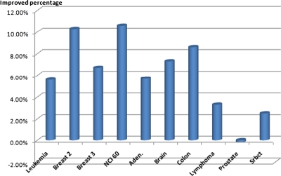
Figure 2 shows the percentage of improvement of the classification error rate for the ten microarray data sets achieved by using the BPSO-CGA method. For Breast 2 class and NCI 60 microarray data, the classification error rates were improved the most, by about 10%. The overall average classification error rate was improved by 7.8% when using the BPSO-CGA method. Only the RF (s.e. = 0) method for the Prostate data set had a lower classification error rate than the proposed method. These results indicate that the proposed method is highly competitive for microarray classification.
FIG. 2.
Improved percentage classification error rates in ten microarray data with BPSO-CGA method.
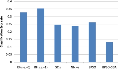
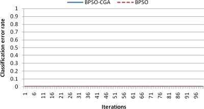
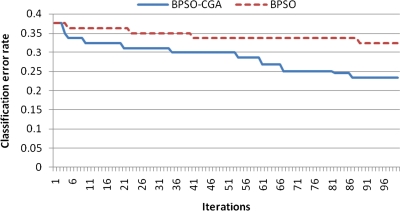
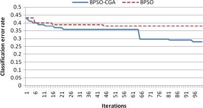
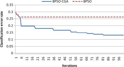
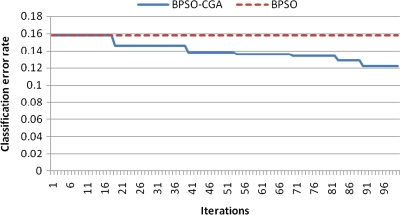
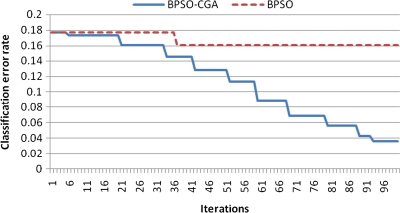
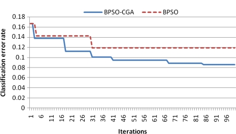
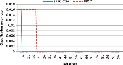
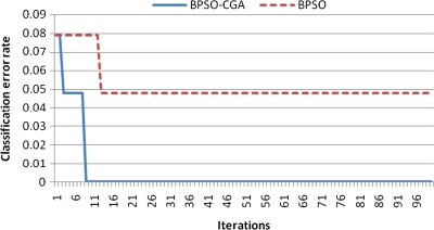
For microarray data, a smaller class should easily achieve a lower classification error rate. Multiclass data sets are usually hard to classify correctly. NCI 60, for example, is a typical multiclass microarray data set, and thus had a higher classification error rate due to its many classes ( = 8). A comparison between other microarray data and NCI 60 shows the proposed method's performance capability for gene selection. Figure 3 shows the NCI 60 microarray data classification error rate for six different methods. The proposed method obtained the lowest classification error rate compared to the four other methods. Figures 4.1 to 4.10 show the number of iterations vs. classification error rate for the ten microarray data sets. After BPSO-CGA feature selection, irrelevant genes will be deleted, thus decreasing the classification error rate and computation time. As shown in Tables 2 and 3, the proposed method could obtain zero classification error rates after gene deletion (Leukemia and Lymphoma data sets), a fact that proves that not all of the genes are relevant for classification.
FIG. 3.
The classification error rate of NCI60 microarray data in six different methods.
FIG. 4.1.
Number of iterations versus classification error rate in Leukemia.
FIG. 4.2.
Number of iterations versus classification error rate in Breast 2 class.
FIG. 4.3.
Number of iterations versus classification error rate in Breast 3 class.
FIG. 4.4.
Number of iterations versus classification error rate in NCI60.
FIG. 4.5.
Number of iterations versus classification error rate in Adenocarcinoma.
FIG. 4.6.
Number of iterations versus classification error rate in Colon.
FIG. 4.7.
Number of iterations versus classification error rate in Brain.
FIG. 4.8.
Number of iterations versus classification error rate in Lymphoma.
FIG. 4.9.
Number of iterations versus classification error rate in Prostate.
FIG. 4.10.
Number of iterations versus classification error rate in Srbct.
3.4. Algorithm analysis
PSO is based on the idea of swarm intelligence in biological populations. BPSO is an information sharing algorithm that randomly generates the initial population for the search process. Each of the particles calculates its position and velocity by neighbor and individual experience. The information is updated based on social interactions between particles. Two independent numbers, rand1 and rand2 in Eq. (1), affect the velocity of each particle. Proper adjustment of the BPSO parameters, such as the inertia weight w and the acceleration factors c1 and c2, is a very important task. The inertia weight w controls the balance between the global exploration and local search ability. A large inertia weight facilitates global search, while a small inertia weight facilitates local search. c1 and c2 control the movement of particles. To avoid premature BPSO convergence, the adjustment should not be changed too excessively, since this might cause particle movement to be erratic and make it impossible to obtain meaningful results. Hence, suitable parameter adjustment is crucial for particle swarm optimization performance. In classical GAs, genes with higher fitness values are retained on the chromosomes, and then other evolutional operators are executed on them. Crossover is the exchange of information between chromosomes, and is the principal element in generating offsprings, i.e., new chromosomes. Reproduction makes copies of the best individuals. Its activity will decrease the performance of the crossover operator, since the latter will have no effect on identical individuals (Erol and Eksin, 2006). The GAs search process moves toward the chromosomes region with higher fitness. This region may be a local optimum region, in which case executing a global search over the entire search space is difficult. In order to prevent this situation from occurring, CGA produce a random number between [0, 1] to generate new chromosomes. The fitness values are calculated from two chromosomes by Eq. (5) and their relative fitness values compared; then the crossover operation is performed. The disadvantages of classic GAs (premature convergence) can be avoided by CGA.
BPSO-CGA is a combination of the BPSO and CGA, two evolutionary methods used to improve the progression of characteristics. In general, pure BPSO can be applied in feature selection and classification problems for microarray data. BPSO has good global search capabilities, but its local search capability is not sufficient. However, when the feature number is high, BPSO results are not good enough. Therefore, we employed a hybridization of BPSO and a CGA. BPSO and CGA both work with the same initial population of solutions, and combining the search abilities of both methods seems to be a reasonable approach. BPSO operates based on knowledge of social interaction, and all individuals are taken into account in each generation. On the other hand, CGA simulates evolution, and some individuals are selected while others are eliminated from iteration to iteration (Kao and Zahara, 2008). These individuals may be regarded as chromosomes in the case of CGA, or as particles in the case of BPSO. A combination of CGA and BPSO executes a local search to progressively improve features. BPSO is thus improves the quality of CGA chromosomes, which in turn leads to better overall solutions. Through the combination of these two different methods, their respective advantages, namely preventing particles from getting trapping (CGA) and search over the entire solution space (BPSO) can both be utilized.
4. Conclusion
Genetic microarray technology has been applied on human life, and using computers to assist in analyzing microarray data is an important topic. In this paper, we propose BPSO-CGA for feature selection, and a K-nearest neighbor (K-NN) with LOOCV serves as an evaluator for gene expression data selection and classification problems. BPSO has good global search capabilities over the entire search space, and the CGA is used for local searches and to optimize the particles of BPSO. The experimental results show that BPSO-CGA leads to a better performance than pure BPSO. The proposed method not only effectively reduced the number of features of ten microarray data sets, but also obtained a lower average classification error rate than four other methods from literature. The obtained results indicate that BPSO-CGA performs well when applied to problems of feature selection and classification.
Acknowledgments
This work was partly supported by the National Science Council in Taiwan (grants NSC94-2622-E-151-025-CC3, NSC94-2311-B037-001, NSC93-2213-E-214-037, and NSC92-2213-E-214-036).
Disclosure Statement
No competing financial interests exist.
References
- AltIncay H. Ensembling evidential k-nearest neighbor classifiers through multi-modal perturbation. Applied Soft Computing. 2007;7:1072–1083. [Google Scholar]
- Berrar D. Bradbury I. Dubitzky W. Instance-based concept learning from multiclass DNA microarray data. BMC Bioinformatics. 2006;7:73. doi: 10.1186/1471-2105-7-73. [DOI] [PMC free article] [PubMed] [Google Scholar]
- Breiman L. Classification and Regression Trees. Chapman & Hall/CRC; Boca Raton, FL: 1984. [Google Scholar]
- Buturovic L.J. PCP: a program for supervised classification of gene expression profiles. Bioinformatics. 2006;22:245. doi: 10.1093/bioinformatics/bti760. [DOI] [PubMed] [Google Scholar]
- Chang J.C. Hilsenbeck S.G. Fuqua S.A.W. The promise of microarrays in the management and treatment of breast cancer. Breast Cancer Res. 2005;7:100. doi: 10.1186/bcr1018. [DOI] [PMC free article] [PubMed] [Google Scholar]
- Choudhary A. Brun M. Hua J., et al. Genetic test bed for feature selection. Bioinformatics. 2006;22:837. doi: 10.1093/bioinformatics/btl008. [DOI] [PubMed] [Google Scholar]
- Cover T. Hart P. Nearest neighbor pattern classification. IEEE Trans. Information Theory. 1967;13:21–27. [Google Scholar]
- Cover T.M. Van Campenhout J.M. On the possible orderings in the measurement selection problem. IEEE Trans. Syst. Man Cybernet. 1977;7:657–661. [Google Scholar]
- Deutsch J.M. Evolutionary algorithms for finding optimal gene sets in microarray prediction. Bioinformatics. 2003;19:45. doi: 10.1093/bioinformatics/19.1.45. [DOI] [PubMed] [Google Scholar]
- Diaz-Uriarte R. de Andres A. Gene selection and classification of microarray data using Random Forest. BMC bioinformatics. 2006;7:3. doi: 10.1186/1471-2105-7-3. [DOI] [PMC free article] [PubMed] [Google Scholar]
- Dudoit S. Fridlyand J. Speed T.P. Comparison of discrimination methods for the classification of tumors using gene expression data. J. Am. Stat. Assoc. 2002;97:77–87. [Google Scholar]
- Eksin I. Erol O.K. Evolutionary algorithm with modifications in the reproduction phase. IEE Proc. Software. 2001;148:75–80. [Google Scholar]
- Erol O.K. Eksin I. A new optimization method: big bang-big crunch. Adv. Eng. Software. 2006;37:106–111. [Google Scholar]
- Fix E. Hodges J.L., Jr. Discriminatory analysis. Nonparametric discrimination: consistency properties. Int. Stat. Rev. 1989;57:238–247. [Google Scholar]
- Forozan F. Mahlamaki E.H. Monni O., et al. Comparative genomic hybridization analysis of 38 breast cancer cell lines: a basis for interpreting complementary DNA microarray data. Cancer Res. 2000;60:4519. [PubMed] [Google Scholar]
- Furey T.S. Cristianini N. Duffy N., et al. Support vector machine classification and validation of cancer tissue samples using microarray expression data. Bioinformatics. 2000;16:906. doi: 10.1093/bioinformatics/16.10.906. [DOI] [PubMed] [Google Scholar]
- Hastie T. Tibshirani R. Friedman J., et al. The elements of statistical learning: data mining, inference and prediction. The Mathematical Intelligencer. 2005;27:83–85. [Google Scholar]
- Holland J.H. Adaptation in Natural and Artificial Systems. MIT Press; Cambridge, MA: 1992. [Google Scholar]
- Hua J. Xiong Z. Lowey J., et al. Optimal number of features as a function of sample size for various classification rules. Bioinformatics. 2005;21:1509. doi: 10.1093/bioinformatics/bti171. [DOI] [PubMed] [Google Scholar]
- Huang H.L. Chang F.L. ESVM: evolutionary support vector machine for automatic feature selection and classification of microarray data. Biosystems. 2007;90:516–528. doi: 10.1016/j.biosystems.2006.12.003. [DOI] [PubMed] [Google Scholar]
- Jeffrey S.S. Lonning P.E. Hillner B.E. Genomics-based prognosis and therapeutic prediction in breast cancer. J. Natl. Comprehensive Cancer Network. 2005;3:291–300. doi: 10.6004/jnccn.2005.0016. [DOI] [PubMed] [Google Scholar]
- Jirapech-Umpai T. Aitken S. Feature selection and classification for microarray data analysis: evolutionary methods for identifying predictive genes. BMC Bioinformatics. 2005;6:148. doi: 10.1186/1471-2105-6-148. [DOI] [PMC free article] [PubMed] [Google Scholar]
- Kao Y.T. Zahara E. A hybrid genetic algorithm and particle swarm optimization for multimodal functions. Appl. Soft Computing. 2008;8:849–857. [Google Scholar]
- Kennedy J. Swarm Intelligence. Springer; New York: 2006. [Google Scholar]
- Kennedy J. Eberhart R. Particle swarm optimization. IEEE Int Conf. Neural Networks. 1995;4:1942–1948. [Google Scholar]
- Kennedy J. Eberhart R.C. A discrete binary version of the particle swarm algorithm. IEEE Int. Conf. Syst. Man Cybernet. 1997;5:4104–4108. [Google Scholar]
- Lee J.W. Lee J.B. Park M., et al. An extensive comparison of recent classification tools applied to microarray data. Comput. Stat. Data Anal. 2005;48:869–885. [Google Scholar]
- Lee Y. Lee C.K. Classification of multiple cancer types by multicategory support vector machines using gene expression data. Bioinformatics. 2003;19:1132. doi: 10.1093/bioinformatics/btg102. [DOI] [PubMed] [Google Scholar]
- Li T. Zhang C. Ogihara M. A comparative study of feature selection and multiclass classification methods for tissue classification based on gene expression. Bioinformatics. 2004;20:2429. doi: 10.1093/bioinformatics/bth267. [DOI] [PubMed] [Google Scholar]
- Liu X. Krishnan A. Mondry A. An entropy-based gene selection method for cancer classification using microarray data. BMC Bioinformatics. 2005;6:76. doi: 10.1186/1471-2105-6-76. [DOI] [PMC free article] [PubMed] [Google Scholar]
- Lonning P.E. Sorlie T. Borresen-Dale A.L. Genomics in breast cancer—therapeutic implications. Nat. Clin. Pract. Oncol. 2005;2:26–33. doi: 10.1038/ncponc0072. [DOI] [PubMed] [Google Scholar]
- Lovbjerg M. Rasmussen T.K. Krink T. Hybrid particle swarm optimiser with breeding and subpopulations. Proc. 3rd Genet. Programm. 2001:469–476. [Google Scholar]
- Oh I.S. Lee J.S. Moon B.R. Hybrid genetic algorithms for feature selection. IEEE Trans. Pattern Anal. Mach. Intell. 2004:1424–1437. doi: 10.1109/TPAMI.2004.105. [DOI] [PubMed] [Google Scholar]
- Ramaswamy S. Tamayo P. Rifkin R., et al. Multiclass cancer diagnosis using tumor gene expression signatures. Proc. Natl. Acad. Sci. USA. 2001;98:15149. doi: 10.1073/pnas.211566398. [DOI] [PMC free article] [PubMed] [Google Scholar]
- Ripley B.D. Pattern Recognition and Neural Networks. Cambridge University Press; New York: 2008. [Google Scholar]
- Sberveglieri M.P.G. Random Forests and nearest shrunken centroids for the classification of sensor array data. Sensors Actuators B Chem. 2008;131:93–99. [Google Scholar]
- Shi Y. Eberhart R. A modified particle swarm optimizer. Proc. IEEE Int. Conf. Evol. Computation. 1998:69–73. [Google Scholar]
- Sorensen K. Sevaux M. MA| PM: memetic algorithms with population management. Computers Operations Res. 2006;33:1214–1225. [Google Scholar]
- Tahir M.A. Bouridane A. Kurugollu F. Simultaneous feature selection and feature weighting using Hybrid Tabu Search/K-nearest neighbor classifier. Pattern Recogn. Lett. 2007;28:438–446. [Google Scholar]
- Tahir M.A. Bouridane A. Kurugollu F., et al. A novel prostate cancer classification technique using intermediate memory tabu search. EURASIP J. Appl. Signal Processing. 2005;14:2241. [Google Scholar]
- Tan S. An effective refinement strategy for KNN text classifier. Expert Syst. Applications. 2006;30:290–298. [Google Scholar]
- Tibshirani R. Hastie T. Narasimhan B., et al. Diagnosis of multiple cancer types by shrunken centroids of gene expression. Proc. Natl. Acad. Sci. USA. 2002;99:6567. doi: 10.1073/pnas.082099299. [DOI] [PMC free article] [PubMed] [Google Scholar]
- Wang X. Yang J. Teng X., et al. Feature selection based on rough sets and particle swarm optimization. Pattern Recogn. Lett. 2007;28:459–471. [Google Scholar]
- Zhu Z. Ong Y. Dash M. Wrapper-filter feature selection algorithm using a memetic framework. IEEE Trans. Syst. Man. Cybernet. B. 2007;37:70. doi: 10.1109/tsmcb.2006.883267. [DOI] [PubMed] [Google Scholar]


