A cross-sample statistical model for SNP detection in short-read sequencing data

Abstract

Highly multiplex DNA sequencers have greatly expanded our ability to survey human genomes for previously unknown single nucleotide polymorphisms (SNPs). However, sequencing and mapping errors, though rare, contribute substantially to the number of false discoveries in current SNP callers. We demonstrate that we can significantly reduce the number of false positive SNP calls by pooling information across samples. Although many studies prepare and sequence multiple samples with the same protocol, most existing SNP callers ignore cross-sample information. In contrast, we propose an empirical Bayes method that uses cross-sample information to learn the error properties of the data. This error information lets us call SNPs with a lower false discovery rate than existing methods.

INTRODUCTION

Highly multiplex sequencing technologies have made DNA sequencing orders of magnitude cheaper; an individual laboratory can now sequence targeted regions of the genome for many individuals at reasonable depth (1). This has dramatically increased our ability to search for single nucleotide polymorphisms (SNPs). To avoid being overwhelmed by false positives when we search for SNPs in large genomic regions, we need to call SNPs in a statistically rigorous way.

Although many studies involve multiple samples prepared and sequenced by the same protocol, current SNP detection methods (2–10) mostly analyze one sample at a time, using sequencing and mapping quality scores to distinguish true SNPs from sequencing and mapping errors. These single-sample methods ignore important cross sample information. Error rates vary across the genome and depend on local DNA content, but they are consistent across samples. True SNPs tend to recur across samples as well. A multisample version of GATK (9,11) sums likelihoods across samples to take advantage of the recurrence of true SNPs but ignores the fact that high error rates are also reproduced across samples. Another existing method, SNIP-Seq (8), uses the consistency of true SNPs and of error rates, but still relies on quality scores. The cross-sample statistical properties of sequencing data have not been extensively explored or used in SNP calling.

In this article, we propose a statistical approach to SNP detection using deep sequencing data from multiple samples. Instead of relying on quality scores, we pool information across samples to estimate the error rate for each position. We do this with an empirical Bayes model that can be fit quickly using a computationally efficient algorithm. Our results show that using cross-sample information efficiently can lead to substantially fewer false discoveries. Since our method uses only the A, C, G, T counts (basewise coverage depth information) for each position and sample, it is not specific to any sequencing technology or data set, and eliminates the substantial computational burden associated with using quality scores.

The intuition behind our approach is simple. Suppose there are N genome positions of interest; for the entire human genome, N is near 3 billion, and for targeted sequencing of selected genomic regions, N can be in the hundreds of thousands. Sequencing yields one N × 4 table of A, C, G, T counts for each sample (as well as other platform-specific information which our method does not use, such as quality scores). We can view SNP calling as a multiple testing problem, where the null hypothesis for each position is that all samples are homozygous for the reference base. If we knew the null distribution of counts at each position—the distribution of base counts if the position were truly homozygous for the reference base—we could apply standard multiple testing ideas to call SNPs and control the false discovery rate of our calls.

It is well known, however, that sequencing and mapping error rates vary substantially across positions (3,6,7). We find that these variations are highly reproducible across samples. Accordingly, we pool information across samples to estimate the null distribution for each position. Figure 1 illustrates this idea. The left simplex shows A, C, G, T frequencies for four homozygous positions with quite different error rates, while the right simplex shows a true SNP position with genotypes GG, GC, CC. If we were to analyze each sample separately, we might falsely conclude that some of the noisier positions were SNPs, since they show high non-reference base frequencies. With a cross-sample model, we can learn the error distribution for each position and distinguish noisy positions from true SNPs.

Figure 1.

The simplex on the left shows four non-polymorphic genome positions of varying degrees of noisiness taken from the example data set, coded by different colors. Within each color, each point is for a different sample. There are two T's (blue and green), one A (yellow) and one G (red). The simplex on the right shows a true SNP that has genotypes C/C, C/G, and G/G among the samples.

We also pool information across genome positions, taking advantage of genome-wide error patterns to improve our null distribution estimates. This can be viewed as a statistical shrinkage estimation method, where the position-specific error distributions are shrunk toward a genome-wide consensus. For most data sets, the number of positions is far greater than the number of positions. For example, the data we use in this article has 300 000 positions and 30 samples. The large number of positions means that any noise property shared across positions can be learned fairly accurately, and thus contribute to the quality of SNP calls. This particularly benefits low-coverage positions, which contain little information in themselves.

Our fundamental idea, pooling data to estimate the null distribution at each position, comes from Efron's empirical null methods for microarray data (12). One of our contributions in this article is extending Efron's ideas to the sequencing setting. Efron's approach is designed for continuous data, and requires a z-score for each hypothesis tested. The SNP detection problem is quite different, since the data is discrete, many positions have very few counts, and the number of counts at each position varies dramatically. We take an empirical Bayes approach similar to Efron's, and use a Dirichlet mixture model to estimate the null distributions efficiently while accounting for the discreteness and depth variation of sequencing data.

MATERIALS AND METHODS

Description of data

In this section, we will summarize important aspects of the data. Unlike existing methods, we take an empirical approach and avoid models tailored toward a specific platform or mapping protocol, so we will largely omit platform specific details.

In a typical sequencing experiment, DNA from the sample of interest is isolated and randomly fragmented, and possibly amplified in a PCR procedure. A fixed number of bases from the ends of the fragments are read by a sequencer, forming a read, that is, a sequence of fixed length from the alphabet  = {A, C, G, T}. The reads are then mapped to a reference genome by an alignment algorithm, yielding {A, C, G, T} counts for each position in the given sample. Different sample preparation protocols, sequencing technologies and alignment methods produce different errors.

As an example, we analyze a collection of 29 normal T cell derived DNA samples. In addition, we also include one sample derived from NA18507, a fully sequenced individual of Yoruban descent (13). In each sample, the coding regions and some nearby intronic regions of 53 genes were selectively enriched as decribed in (14) and (15). The targeted region was recovered in the form of 1157 double stranded linear amplicons covering 309Kb. This material was concatenated and mechanically fragmented in order to avoid overrepresentation of amplicon ends. Sequencing libraries were prepared from this material and sequenced following established procedures (see the Supplementary Data for more details).

Our analysis focuses on the array of {A, C, G, T} counts to avoid being tied to any particular sample preparation, sequencing or alignment technique. We call the number of reads that contain a given position the coverage of that position. The coverage varies substantially across positions because of random errors introduced at each stage of the sequencing process and the influence of the local genomic environment.

The error rate also varies substantially across positions. As discussed in earlier reports (3,6,7), there are many sequence-specific features that contribute to this variation. For example, some genomic regions are more repetitive than others, and are thus more prone to alignment errors. Certain combinations of DNA bases can also lead to higher sequencing error.

These causes of increased error rates depend on the genome environment, which to a large extent does not vary between samples. We thus expect the error rate for a given position to be consistent across samples that are prepared, sequenced and mapped using the same protocol. Figure 3 in the ‘Results’ section shows that this is indeed true for our data. The reproducibility of error rates suggests that we can estimate and correct for positional error rate variation through a cross-sample model.

Figure 3.

Error rates for sample 1 (x axis) and 2 (y axis), plotted on a log-log scale. The left plot shows the errors for all genome positions, while the right one only shows the errors for high-coverage positions (at least 10 000 in each sample). The reduced variability in the right plot illustrates how most of the variability in observed error rates actually comes from binomial noise, because of the low depth. Points with no error are not shown.

Error rates also show genome-wide patterns. For example, in our data, C is globally more likely to be misread as A than as T. These global error patterns can help us estimate the error rate for low-coverage positions, since the small number of counts at these positions make even the cross-sample error estimates unreliable.

Dirichlet mixture model

We frame SNP detection as a multiple hypothesis testing problem in order to detect SNPs in a statistically rigorous way. We want to test N null hypotheses, where the i-th null hypothesis is that position i is homozygous for the reference base in all of the samples. Since most positions in the human genome are non-polymorphic, most positions in any data set will be null. To test these hypotheses rigorously, we need to learn the appropriate null and alternative distributions at each position.

We propose an empirical Bayes mixture model that shares information across samples and positions to efficiently estimate these distributions. We use the following generative model for the counts of the four bases at each position. First, for each position i, a null frequency vector and an alternative frequency vector are generated from null and alternative priors _null and _alt, repectively. Next, each sample is assigned to the null or alternative: indicators δ_ij are generated for each sample j at each position i, assigning the sample to the null (δ_ij = 0) or the alternative (δ_ij = 1) at the position. Finally, counts for each sample are generated from the appropriate multinomial distribution, using the observed coverage N_ij and either the null (p_i) or the alternative (q_i) frequency vectors. Expressed mathematically, this gives the following model for position i:

Figure 2 shows a diagram of this model.

Figure 2.

Our model, displayed in graphical model plate notation. The boxes denote generation of a quantity for each position and each sample. We display (1 − δ)p + δq as ‘r’ for brevity.

With this model, we proceed in three steps. We first estimate _null, _alt, π_i, p_i and q_i by maximum likelihood using a modified EM algorithm detailed in the Supplementary Data. We then use the estimated parameters to find the posterior probability that each position is homozygous for the reference base in each sample (that is, we find E(δ_ij|X)). Last, we use the estimated posterior probabilites to call SNPs. Estimating the priors _null, _alt lets us share information across positions, and estimating the non-null probability π_i and the position specific null and alternative frequency vectors p_i and q_i lets us share information across samples.

In the rest of this section, we explain our modeling approach in more detail. Our fitting algorithm is a modified EM algorithm. It is reasonably fast; fitting our model for our 300 000 position, 30 sample example data set takes about 25 min on a 1.6 Ghz computer with 2 Gb RAM. The algorithm is easily paralellizable as well. We defer the full details of our fitting algorithm to the Supplementary Data.

We model the priors _null and _alt as G component Dirichlet mixtures:

Mixture models give us convenient conjugate priors, but with the flexiblity to adapt to many different error distributions.

To estimate _null and _alt more efficiently, we impose extra constraints on the mixture parameters. First, we require that all the Dirichlets have the same precision . Second, we choose our mixture components to take advantage of the structure of SNP data. The simplest version of our approach would be to use four null components (one each of homozygous {A, C, T, G}), and six alternative components (one for each heterozygous combination of {A, C, G, T}). Geometrically, the null components put probability near the corners of the {A, C, G, T} simplex, while the alternative components put probability near the edge midpoints. We require that the null mixture probabilities θ_null,g be non-zero only on the null components and the alternative mixture probabilities θ_alt,g be non-zero only on the alternative components.

This basic approach, however, does not fit our data well. In our data, we found that nearly all positions are ‘clean’, with very low error rate, but a small proportion are ‘noisy’, with a much higher error rate. The noisy positions often reside in repetitive regions that are hard to map. This error rate distribution is not modeled well by a single Dirchlet group for each corner and edge midpoint of the simplex, but is well modeled by a mixture of two Dirichlets in each corner and edge midpoint. This gives us 8 null and 12 alternative mixture components.

Our algorithm does not explicitly model the possibility that a position is homozygous for a non-reference base. Instead, our fitting procedure is such that each position is very likely to have a null distribution generated from the homozygous group corresponding to the reference base. This means that if a position is homozygous for a non-reference base, it will strongly appear to have been generated from an alternative group, and will thus be correctly called as a SNP. For example, suppose the reference base for a position is C and a position is homozygous AA in a given sample. The position is far more likely to have been generated from the AC alternative than the CC null, so even though our model does not explicitly consider the possiblity that the position is AA, we will still detect it as a SNP. We re-genoytpe all called positions in post-processing, so all that matters is that this step of our algorithm makes the right SNP calling decision.

Since the data contains so many positions and most positions are null, we can expect the fitted null parameters to be quite accurate. But since SNPs are rare, our data will typically contain few positions displaying each heterozygous genotype. This makes the alternative mixture components very difficult to estimate. We solve this issue by constraining the alternative Dirichlet parameters α_g. We require α_g for the heterozygote groups g ∈ {AC, AG, AT, CG, CT, GT} to be equal to the averages of their corresponding homozygote groups. For example,

This constraint significantly stabilizes the parameter and FDR estimates.

Calling, filtering and genotyping

Given our parameter estimates and posterior estimates of δ_ij, we call SNPs as follows. We estimate the positional false discovery rate, the posterior probability that all of the samples for a position are homozygous for the reference base:

We estimate fdr by taking a weighted product of the estimated δ_ijs, downweighting very low-coverage positions:

We use weights w_ij = max((N_ij − 3)₊, 20). This gives samples with coverage less than three no weight, since these are particularly noisy in our data, and saturates the weights at an arbitrary depth of 23, since increasing N beyond such coverage does not make δ more accurate. Given the estimated fdr, we make a list of putative SNPs with low (we used a threshold of 0.1).

We then fit a mixture model by maximum likelihood to genotype the called positions. First, we reduce the counts to the reference and highest non-reference base counts; suppose for concreteness that these are A and C, respectively. This produces a M × 2 count matrix Y for each putative SNP, with each row Y_j corresponding to one sample. Next, we fit the following generative model for Y_j: each sample Y_j is first assigned a genotype g_j with probability p = (p_AA, p_AC, p_CC). The non-reference base counts are then binomial, 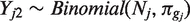, where N_j is the depth for sample j and π_g is the expected non-reference proportion for the assigned genotype. For example, if the reference base is A, π_AA is the probability of error, and π_AC would would ideally be 0.5 but is typically lower due to mapping bias.

We use the EM algorithm to fit this model under the Hardy-Weinberg restriction that . This restriction can be removed for populations where the Hardy–Weinberg model does not apply. We constrain π_g so the homozygous types have π near 0 and 1, and the heterozygous types have π near 0.5. The estimated group membership indicators from the EM algorithm give us estimated genotypes for each sample at the position.

This calling procedure assumes we are interested in detecting SNPs. If we are interested in detecting nonreference positions in particular samples, we can look at the Hardy–Weinberg genotype results, or simply consider the estimated indicators δ_ij from the mixture model. Although they do not distinguish between heterozygosity and homozygosity for a non-reference base, the δ_ij are typically more accurate indicators of SNP status than the Hardy–Weinberg genotypes for very low-depth samples. For the single-sample comparison in the results, we detect SNPs as above, using , then detect SNPs in the sample of interest using the genotypes, but require that δ_ij ≥ 0.9 for low depth (N ≤ 4) positions.

An estimator of the false discovery proportion

Assessing SNP calls is difficult since we do not know the true SNP status of most positions. We propose a simple nonparametric way to estimate the false discovery proportion (FDP) for a set of calls in a single sample, which we use to evaluate the accuracy of different SNP calling methods. A specific instance of this estimator justifies the use of the Ti/Tv ratio, a popular assessment metric for SNP callers.

Our method is based on a simple general inequality. Consider a set of candidate SNP positions. Let Z_i be a random variable that is observed for each candidate position i ∈ . Let H_i be the event that position i is actually null, and let

be the FDP for this candidate set. Suppose we know that

(1)

with a < b. Then

and hence

(2)

If a and b are upper bounds for the conditional expectations in Equation 1, then the right side of Equation 2 is an upper bound on η.

If we have such a quantity Z_i, we can estimate μ using the data,

and use Equation 2 to estimate the FDP η. If we know a and b exactly, we obtain an unbiased estimate of the FDP, and if we have upper bounds on a and b, we obtain an estimated upper bound on the FDP.

The key to applying this result is to choose a variable Z_i for which we can estimate a and b accurately. This can be difficult because the expectations in (1) are conditioned on the rejection set . Ideally, we would choose a Z_i such that conditional on H_i, Z_i is independent of the event {i ∈ }. We would then have a = E[Z_i|H₀], b = E[Z_i|H₁], and we could estimate these quantities from a training set consisting of known null and non-null positions.

This conditional independence property also makes it easier to compare different SNP calling methods. Suppose two methods yield two sets of candidate SNP positions ₁, ₂ of candidate SNP positions. If Z_i were independent of both {i ∈ R₁} and {i ∈ R₂} conditional on H_i, then a and b would be the same for the two methods, and we could compare their accuracy using directly. This lets us avoid using possibly inaccurate estimates of a and b.

Exact conditional independence of Z and the event of rejection is often hard to achieve, especially since Z must also be chosen so that we have the inequality a < b. However, there are cases where approximate independence can be assumed. This assumption must be carefully evaluated for each study where this FDP estimator is applied.

Ti/Tv ratio

The ratio of the number of transitions (Ti) to the number of transversions (Tv) is often used to measure specificity for SNP discovery methods. Null positions should have a Ti/Tv ratio of 0.5, since there are twice as many transversions as transitions. What makes the Ti/Tv ratio useful is that its value for true SNP positions has been empirically observed to be much higher than 0.5. Recent studies from the 1000 genomes project shows that Ti/Tv is around 2–2.1 for the whole human genome, but can be ≥3.0 in exomes.

In our notation, this approach is equivalent to letting Z_i be the indicator of the event that a mutation from the most frequently observed base to the second most frequently observed base at position i is a transition. Using Ti/Tv relies on the assumption that the SNP caller is not biased toward calling any base pair combination as heterozygote. Although this assumption is never exactly true, the biases of the SNP caller are usually small enough for the Ti/Tv ratio to be informative.

Coverage biases between alleles

We now construct a new Z_i for which we can estimate a and b. For a given position i, define b_i to be the reference base and to be the non-reference base with highest coverage. That is, suppressing the sample indicator j in our notation, . We then let

be the event that the coverage of b_i is lower than the coverage of .

Consider the case where i is a truly heterozygous position. Assuming that one of the two alleles is the reference base, the probability P(Z_i = 1) should ideally be 1/2, if the experiment does not favor either base. In most cases, the final mapping step is biased toward throwing away reads containing the non-reference base, making the probability b in (1) slightly <0.5.

Now consider the case where i is a homozygous position that has been falsely declared to be heterozygous. Usually, this happens because the coverage of is higher than would be expected under random error. Even so, we found empirically that it is extremely rare for the high error rates to be greater than 0.5. That is, even when the error rate is high enough to generate a false positive, the event Z_i = 1 is still rare enough that the probability a in (1) is close to zero. Thus, we make the approximation a ≈ 0 which leads to

(3)

Let b₀ = P(Z_i|H_i = 1). By Bayes rule, we have

(4)

We assume that the method rejects the null if Z_i = 1, i.e.

(5)

We found this to be a good approximation for all of the methods compared (see ‘Results’ section).

Substituting (5) into the numerator of the right hand side of (4) yields

(6)

where β ≡ P(i ∈ |H_i = 1) is the recall rate of the method, which can be estimated on a training set of known heterozygous positions. Substituting (6) into (3), we have

(7)

with each component of the above formula estimable from data.

RESULTS

Coverage and error rate variation

We find that the coverage and error rates vary substantially across positions, and that the error rate is reproducible across samples. In our data, the coverage spanned five orders of magnitude, ranging from 0 to over 100 000, and was reproducible across samples (Figure 1 in the Supplementary Data). Although the error rate varies substantially across positions, it is consistent across samples. Figure 3 plots each position's error rate in one of the samples across its error rate in another. The consistency of the positional error rates across samples justifies estimating them using a cross-sample model.

SNP calling results

Results on 53 gene data set

We used our method on the data from 53 genes and 30 samples, which includes the sample NA18507. We also applied SNIP-seq (8) and GATK (9,11) Multi-sample on this data set, and GATK single sample on NA18507 alone. Both GATK and SNIP-seq use quality scores. To assess the impact of using quality scores on our method, we also ran our method on quality score filtered depth charts. Details on our use of GATK and our quality score filtering are in the Supplementary Data.

To assess recall, we found the overlap of each method's calls with the SNPs identified by Bentley et al. (13). To eliminate possible false positives in the calls made by Bentley et al. (13), we restrict our attention to the calls they make that appear in dbSNP. Also, to assess algorithmic power and not experimental power, we ignore SNP calls made by Bentley et al. (13) and dbSNP that had very little coverage in our data (3 or fewer reads in the unfiltered counts).

To assess the precision of the SNP callers, we use two methods: the standard Ti/Tv ratio and the newly proposed non-parametric FDP estimator based on the proportion of times where highest non-reference base frequency is higher than the reference base frequency (PNRH). The PNRH on the calls made by Bentley et al. (13) filtered by dbSNP was 0.611, while its value for the rest of the positions was 0.0007. Figure 4 shows that PNRH of our call set drops consistently as we lower the calling threshold.

Figure 4.

Decline in proportion of calls with non-reference base frequency higher than reference base frequency as the number of calls increase.

This empirical evidence indicates that PNRH reflects the enrichment of true SNPs in a call set. To compute the FDP from the PNRH, we used b₀ = 0.611, which was computed from the set of SNPs in (Bentley et al. (13) ∩ dbSNP). The percentage of Bentley positions called is used as the value of β for each method. To check assumption (5), we focused on the set of positions called by Bentley et al. that is also in snpDB, and filtered by the observable characteristic Z_i = 1. On this filtered set, the proportion that is called is >0.99 for all methods but GATK Multisample. GATK Multisample called 90% of the positions. Thus, we added a multiplier of 0.9 to the right hand side of the formula (6) for b for GATK Multisample.

Tables 1 and 2 show the results. All the methods have about similar recall (the recall of GATK is slightly lower), but they make dramatically different precision tradeoffs to achieve that recall. SNIP-Seq makes many more calls than our method, and its calls have low precision—its novel calls have an estimated FDP of 63.4%. GATK makes fewer calls, but both its single-sample and multi-sample modes have a high estimated FDP on their novel calls, 37.3 and 41.9%, respectively. Our methods' novel calls are much more precise, with an estimated FDP of 29.6% (28.0% after filtering by quality score). Accordingly, the PNRH is highest for our method, and lower for the other existing methods.

Table 1.

Calls on the Yoruban sample by various methods, with estimated FDPs

Method	Our method	Our method, quality > 20	SNIP-Seq	GATK single-sample	GATK multi-sample
Positions called	623	622	1088	491	475
Bentley positions called (out of 238)	227	228	228	217	208
Percentage bentley positions called (%)	95.4	95.8	95.8	91.2	87.4
Estimated FDP of all calls (%)	15.0	14.8	48.0	15.7	21.0
Estimated FDP of new calls (%)	29.6	28.0	63.4	37.3	41.9

Table 2.

Proportion of calls where highest non-reference base frequency is higher than reference base frequency (PNRH) and Ti/Tv ratios for the various sets of calls

Method	Bentley et al. (13) ∩ snpDB	Our method	Our method, quality > 20	SNIP-Seq	GATK single-sample	GATK multi-sample
PNRH (all calls)	0.611	0.520	0.521	0.318	0.515	0.483
Ti/Tv ratio (all calls)	2.31	2.03	2.03	1.20	1.81	1.55
PNRH (new calls)	–	0.449	0.453	0.234	0.400	0.371
Ti/Tv ratio (new calls)	–	1.88	1.88	1.02	1.49	1.12

The PNRH and Ti/Tv ratios were calculated on all calls and on new calls [calls not in (Bentley et al. (13) ∩ dbSNP)].

The same conclusion is reached if we use the Ti/Tv ratio: it is highest for the validation set of Bentley et al. (13) calls that appear in dbSNP, at value 2.31. The set of calls made by our method has a Ti/Tv ratio of 2.03, which is not improved upon by quality filtering. The other methods have much lower Ti/Tv ratios, at 1.20 (SNIP-Seq), 1.81 (GATK Single-sample) and 1.55 (GATK Multisample).

The multi-sample version of GATK seems less precise than the single-sample version, by both the FDP and the Ti/Tv ratio. This is probably because, by simply summing the position wise likelihoods across samples, GATK Multisample strengthens reproducible artifacts in noisy positions and falsely calls them as SNPs.

Quality score filtering has very little effect on our method's precision and recall. This indicates that our method can indeed use cross-sample information to learn the error properties of the data that would otherwise have been obtained from quality scores. Replacing quality scores with empirical cross sample modeling can yield substantial computational savings and portability.

Both the Ti/Tv and FDP comparisons lead to the same comclusion: our method is much more precise than and at least as powerful as SNIP-Seq and both versions of GATK.

Spike-in experiment results

A spike-in simulation also shows that our method has good power on this data. We simulated SNP data and added it to our experimental data. We took a clean null position or a noisy null position and replaced the samples with counts corresponding to SNPs, row by row starting at the top (the original counts for the positions are in the Supplementary Data). The SNP rows were (x, 0, n − x, 0), where n is the assumed coverage for the SNP and .

Figure 5 shows the spike-depth n needed to call a SNP with 80% power with fdr ≤ 0.1. Because our method borrows information across samples, the power depends on the number of heterozygous samples. The depth required to call the SNP falls quickly as the number of heterozygous samples increases. If two or more samples are heterozygous at a clean position, our method only needs a depth of seven to achieve good power (eight at a noisy position).

Figure 5.

Coverage needed for 80% power at fdr ≤ 0.1 for clean and noisy positions. The coverage needed for noisy positions at 28 heterozygous samples increases because our algorithm begins considering that position extremely noisy at that stage.

Model-based simulation

Finally, we investigated the fdr estimation accuracy of our procedure with a parametric simulation, presented in the Supplementary Data. In brief, these simulations show that our method can conservatively estimate the true fdr when the data is generated from the model we are fitting. This test validates our fitting method, which is important, since we are maximizing a non-convex likelihood with many local optima.

CONCLUSION

In this article, we introduced an empirical Bayes method that learns the error properties of sequencing data by pooling information across samples and positions. Our method uses mixture models to extend Efron's empirical null ideas (12) to sequencing data in a computationally and statistically efficient way. By borrowing information across samples and positions, we are able to detect SNPs with fewer false discoveries than existing methods, without sacrificing power.

As sequencing-based variant detection moves beyond the proof-of-principle stage, statistical methods for false discovery control become necessary for large-scale studies. We have adapted empirical Bayes methods to this problem, and showed that error information can be reliably learned from the count tables, without relying on platform specific models. This approach can be useful for other types of sequencing applications, such as finding somatic mutations in matched tumor and normal tissues and detecting emerging quasi-species in virus samples. Finding the best way to pool information in each setting is an important direction for future research.

SUPPLEMENTARY DATA

Supplementary Data are available at NAR Online: Supplementary Tables 1–3, Supplementary Figures 1 and 2, Supplementary Sections 1–3 and Supplementary References [1–4].

FUNDING

National Institutes of Health (NIH) (5K08CA968796 to H.P.J., DK56339 to H.P.J, 2P01HG000205 to J.D.B, J.M.B. and H.P.J., R21CA12848 to J.M.B. and H.P.J., R21CA140089 to H.P.J. and G.N. and RC2 HG005570-01 to G.N., H.X., J.M.B. and H.P.J.); I.K. was supported by the Lymphoma and Leukemia Society; National Science Foundation (NSF) VIGRE Fellowship (to O.M.); National Library of Medicine (T15LM007033 to D.N.); NIH (R01 HG006137-01); NSF DMS (Grant 1043204 to N.R.Z.); Doris Duke Clinical Foundation (to H.P.J.), Reddere Foundation (to H.P.J.), the Liu Bie Ju Cha and Family Fellowship in Cancer (to H.P.J.), the Wang Family Foundation (to H.P.J.) and the Howard Hughes Medical Foundation (to H.P.J.). Funding for Open access charge: NSF.

Conflict of interest statement. None declared.

REFERENCES

- 1.Shendure J, Ji H. Next-generation DNA sequencing. Nature Biotechnol. 2008;26:1135–1145. doi: 10.1038/nbt1486. [DOI] [PubMed] [Google Scholar]
- 2.Li H, Ruan J, Durbin R. Mapping short DNA sequencing reads and calling variants using mapping quality scores. Genome Res. 2008;18:1851–1858. doi: 10.1101/gr.078212.108. [DOI] [PMC free article] [PubMed] [Google Scholar]
- 3.Van Tassell CP, Smith TP, Matukumalli LK, Taylor JF, Schnabel RD, Lawley CTT, Haudenschild CD, Moore SS, Warren WC, Sonstegard TS. SNP discovery and allele frequency estimation by deep sequencing of reduced representation libraries. Nature Methods. 2008;5:247–252. doi: 10.1038/nmeth.1185. [DOI] [PubMed] [Google Scholar]
- 4.Ossowski S, Schneeberger K, Clark RM, Lanz C, Warthmann N, Weigel D. Sequencing of natural strains of Arabidopsis thaliana with short reads. Genome Res. 2008;18:2024–2033. doi: 10.1101/gr.080200.108. [DOI] [PMC free article] [PubMed] [Google Scholar]
- 5.Holt KE, Teo YY, Li H, Nair S, Dougan G, Wain J, Parkhill J. Detecting SNPs and estimating allele frequencies in clonal bacterial populations by sequencing pooled DNA. Bioinformatics. 2009;25:2074–2075. doi: 10.1093/bioinformatics/btp344. [DOI] [PMC free article] [PubMed] [Google Scholar]
- 6.Hoberman R, Dias J, Ge B, Harmsen E, Mayhew M, Verlaan DJ, Kwan T, Dewar K, Blanchette M, Pastinen T. A probabilistic approach for SNP discovery in high-throughput human resequencing data. Genome Res. 2009;19:1542–1552. doi: 10.1101/gr.092072.109. [DOI] [PMC free article] [PubMed] [Google Scholar]
- 7.Li R, Li Y, Fang X, Yang H, Wang J, Kristiansen K, Wang J. SNP detection for massively parallel whole-genome resequencing. Genome Res. 2009;19:1124–1132. doi: 10.1101/gr.088013.108. [DOI] [PMC free article] [PubMed] [Google Scholar]
- 8.Bansal V, Harismendy O, Tewhey R, Murray SS, Schork NJ, Topol EJ, Frazer KA. Accurate detection and genotyping of SNPs utilizing population sequencing data. Genome Res. 2010;20:537–545. doi: 10.1101/gr.100040.109. [DOI] [PMC free article] [PubMed] [Google Scholar]
- 9.McKenna A, Hanna M, Banks E, Sivachenko A, Cibulskis K, Kernytsky A, Garimella K, Altshuler D, Gabriel S, Daly M, et al. The Genome Analysis Toolkit: a MapReduce framework for analyzing next-generation DNA sequencing data. Genome Res. 2010;20:1297–1303. doi: 10.1101/gr.107524.110. [DOI] [PMC free article] [PubMed] [Google Scholar]
- 10.Li R, Li Y, Kristiansen K, Wang J. SOAP: short oligonucleotide alignment program. Bioinformatics. 2008;24:713–714. doi: 10.1093/bioinformatics/btn025. [DOI] [PubMed] [Google Scholar]
- 11.DePristo M, Banks E, Poplin R, Garimella K, Maguire J, Hartl C, Philippakis A, delAngel G, Rivas M, Hanna M, et al. A framework for variation discovery and genotyping using next-generation DNA sequencing data. Nature Genet. 2011;43:491–498. doi: 10.1038/ng.806. [DOI] [PMC free article] [PubMed] [Google Scholar]
- 12.Efron B. Large-scale simultaneous hypothesis testing: the choice of a null hypothesis. J. Am. Stat. Assoc. 2004;99:96–104. [Google Scholar]
- 13.Bentley DR, Balasubramanian S, Swerdlow HP, Smith GP, Milton J, Brown CG, Hall KP, Evers DJ, Barnes CL, Bignell HR. Accurate whole human genome sequencing using reversible terminator chemistry. Nature. 2008;456:53–59. doi: 10.1038/nature07517. [DOI] [PMC free article] [PubMed] [Google Scholar]
- 14.Dahl F, Stenberg J, Fredriksson S, Welch K, Zhang M, Nilsson M, Bicknell D, Bodmer WF, Davis RW, Ji H. Multigene amplification and massively parallel sequencing for cancer mutation discovery. Proc. Natl Acad. Sci. USA. 2007;104:9387–9392. doi: 10.1073/pnas.0702165104. [DOI] [PMC free article] [PubMed] [Google Scholar]
- 15.Natsoulis G, Bell JM, Xu H, Buenrostro JD, Ordonez H, Grimes S, Newburger D, Jensen M, Zahn JM, Zhang N, et al. A flexible approach for highly multiplexed candidate gene targeted resequencing. PLoS ONE. 2011;6:e21088. doi: 10.1371/journal.pone.0021088. [DOI] [PMC free article] [PubMed] [Google Scholar]
Associated Data
This section collects any data citations, data availability statements, or supplementary materials included in this article.