Abstract
Nonlinear partial differential equation (PDE) models are established approaches for image/signal processing, data analysis and surface construction. Most previous geometric PDEs are utilized as low-pass filters which give rise to image trend information. In an earlier work, we introduced mode decomposition evolution equations (MoDEEs), which behave like high-pass filters and are able to systematically provide intrinsic mode functions (IMFs) of signals and images. Due to their tunable time-frequency localization and perfect reconstruction, the operation of MoDEEs is called a PDE transform. By appropriate selection of PDE transform parameters, we can tune IMFs into trends, edges, textures, noise etc., which can be further utilized in the secondary processing for various purposes. This work introduces the variational formulation, performs the Fourier analysis, and conducts biomedical and biological applications of the proposed PDE transform. The variational formulation offers an algorithm to incorporate two image functions and two sets of low-pass PDE operators in the total energy functional. Two low-pass PDE operators have different signs, leading to energy disparity, while a coupling term, acting as a relative fidelity of two image functions, is introduced to reduce the disparity of two energy components. We construct variational PDE transforms by using Euler-Lagrange equation and artificial time propagation. Fourier analysis of a simplified PDE transform is presented to shed light on the filter properties of high order PDE transforms. Such an analysis also offers insight on the parameter selection of the PDE transform. The proposed PDE transform algorithm is validated by numerous benchmark tests. In one selected challenging example, we illustrate the ability of PDE transform to separate two adjacent frequencies of sin(x) and sin(1.1x). Such an ability is due to PDE transform’s controllable frequency localization obtained by adjusting the order of PDEs. The frequency selection is achieved either by diffusion coefficients or by propagation time. Finally, we explore a large number of practical applications to further demonstrate the utility of proposed PDE transform.
Keywords: Mode decomposition, Evolution equations, Anisotropic diffusion, Total variation, High-pass filter, Partial differential equation transform
I Introduction
Processing and analysis of signal, sound, data, image, surface or video frame have been an important issue in a general category of subjects, including computer vision, face recognition, feature detection, medical diagnosis, remote sensing, machine vision, and artificial intelligence.13,20,47,51 Signal, image, surface and data processing are realized via a family of operations and algorithms, such as filtering, smoothing, denoising (or deblurring), enhancement, segmentation, reconstruction, pattern recognition, surface analysis and construction. The advance in signal, image, surface and data analysis also benefits many related fields, such as optical sorting, automatic control, augmented reality, robotics, sonar, radar, communication, navigation, biomolecular modeling and a variety of imaging modalities. There are a variety of algorithms for signal, image, surface and data processing. The essential idea is the use of filters, such as linear, nonlinear, active, passive, low-pass, high-pass, Fourier, wavelet, Chebyshev, Gaussian, Kalman, Wiener and conjugate filters.27,52,53,69 Decomposition of the original signal, image, surface and data into various modes according to their mathematical features and frequency distributions is a key procedure in all the aforementioned applications. Usually, the subsequent analysis, also called secondary processing, on individual mode components enables us to achieve our goal of signal, image, surface and data analysis. Therefore, mode decomposition is a fundamental process in information processing and data analysis.
Fourier or spectral analysis is a classical technique for mode decomposition and remains to be a powerful tool in signal, image and data processing.13,36,42,51,55 However, Fourier analysis is not suitable for studying data of non-stationary nature, and it may be difficult to choose a suitable window size to satisfy the conflicting requirements of localizing an event in time and resolving its frequency distribution. Moreover, the method is not data adaptive. In many applications in signal processing, one usually desires the information of detailed position and momentum relation, which is also lack in Fourier spectral analysis. Besides, Fourier analysis is less ideal for applications in image processing when localized visual features like edges need to be detected. Most importantly, when the signal or image involves abundantly many modes, the subsequent analysis or secondary processing becomes awkward if it is not fully automatic.
Wavelet transform is another popular technique for mode decomposition and shows a great power in analyzing unsteady and non-stationary data.13,17,20,28,33,39,40,51,60 The fundamental idea behind wavelet filters is to analyze data according to their scales. In this sense, wavelets realize the locality by resorting to localized multiscale bases, which are usually more appropriate than sines and cosines in the Fourier basis, and decomposing signal into various sub-bands. Since individual wavelet functions can be localized in space while Fourier sine and cosine functions are not, many functions become “sparse” in wavelet bases. By dilation and translation, wavelet transform usually yields much fewer number of non-trivial sub-bands than the number of Fourier modes, and thus results in many useful applications such as data compression, detecting features in images, and removing noise from time series. Wavelet methods thus provide an efficient approach for image mode decomposition and secondary processing. Most modes separated by wavelet transform are usually closely related to the edge information or global feature of the whole image. Therefore, wavelets are efficient for image compression. Overall, the wavelet methods are more adaptive than Fourier analysis. However, wavelet analysis is basically a linear analysis and suffers from many limitations. The down sides include uniformly poor resolution, sometimes counter-intuitive interpretation, and non-data adaptive nature as the same wavelet basis is used to analyze all the data.30 Moreover, wavelet methods inherit many drawbacks of the Fourier analysis since many commonly used wavelets were originated from Fourier analysis.
Witkin introduced the diffusion equation for image denoising in 1983.63 The central idea is that the evolution of an image under a diffusion operator is formally equivalent to the standard Gaussian low-pass filter, which is commonly used for image denoising. In 1990, Perona and Malik proposed an anisotropic diffusion equation44 which is able to remove noise without smearing the image edges too much. In the anisotropic diffusion equation, the diffusion coefficient is replaced by a function of image gradients such that the diffusion coefficient is small at the image edges.11,44,50,59,61 Therefore, the Perona-Malik equation is nonlinear. Despite of better image edge protection, the nonlinear anisotropic diffusion operator may break down when the gradient generated by noise is comparable to image edges and features.8,41 Application of a pre-convolution with a smoothing function to the image can practically alleviate the instability and reduce grey scale oscillation, but the image quality is often degraded. One alternative solution introduced by Wei59 is to statistically discriminate noise from image edges by a measure based on the local statistical variance of the image. Such a local statistical variance based edge-stopping algorithm works very well for image restoration. An advantage of this anisotropic diffusion approach is that geometric properties, such as curvature, can be easily embedded in partial differential equation (PDE) operators to achieve desirable effects in image and surface. The level set method devised by Osher and Sethian is a typical example of using the mean curvature flow for image43,46,48 and surface analysis.3 For this reason, this class of nonlinear evolution equations is also called geometric PDEs or geometric flows. Mathematically, the study of geometric PDEs has enormous impact on geometry analysis, manifold theory, topology, geometric measure theory, and certainly PDEs. In the past two decades, PDE based image processing approaches have raised a strong interest in the mathematical community and have opened new approaches for image de-noising, enhancement, edge detection, restoration, segmentation, etc.1,3,4,7,25,32,35,45,47,49,64 Recently, geometric PDEs have been utilized as a means for the molecular surface construction of macromolecules3 and the multiscale modeling of nano-bio systems.15,16,58
Variational method is a most powerful mathematical tool. Total variation based edge-preserving image restoration models were pioneered by Rudin, Osher, and Fatemi.46 The variational PDE technique has been widely used in numerous applications such as image segmentation,6,12,67 restoration,46 compression,19 and image inpainting.10 The growing impact of variational PDE techniques in image processing is mainly due to their capability of controlling the geometrical features of images and data. The essential idea is that signals and images with extra and possibly spurious components have a relatively large variation or gradient. As such, image processing can be formulated as a problem of minimizing the total energy defined as a functional of the gradient of the image, while preserving important image contents such as edges. The minimization of the total energy by the Euler-Lagrange equation leads to a mean curvature term which helps retain sharp edges in image restoration. Central to most variational PDE methods, the goal of the total energy variation is to reconstruct an image with the best fidelity and the least noise. Regularization procedures and PDE analysis are usually employed in total variation models.9
Both the Perona-Malik equation44 and earlier total variation models employ second order nonlinear PDEs for image or surface analysis. The Willmore flow, proposed in 1920s, is a fourth order geometric PDE and has also been used for surface analysis. In 1999, Wei introduced the first family of arbitrarily high order nonlinear PDEs to more efficiently remove image noise in edge-preserving image restoration.59 The same research group also proposed an arbitrarily high order geometric PDE for the surface formation and evolution of protein and other molecules.2 In the past decade, high order nonlinear PDEs, particularly fourth order nonlinear PDEs, have attracted much attention in image analysis.2,9,11,23,24,38,54,59,68 Compared with second order PDEs, the higher order PDEs are able to suppress high frequency components, including noise, at fast rates. Mathematical analysis of fourth order nonlinear PDEs in Sobolev space was carried out by Bertozzi and Greer,5,23,24 who proved the existence and uniqueness of the solution to a case with H1 initial data and a regularized operator. Xu and Zhou65 performed similar analysis. Recently, Jin and Yang have proved the existence of the strong solution of Wei’s fourth order equation, which is in fact mathematically different from other fourth order PDEs.34 In general, however, high order PDEs are subject to strict stability constraints in their numerical solutions. Witelski and Bowen designed alternating-direction implicit (ADI) schemes for high order nonlinear PDEs.62 ADI and other implicit approaches are particularly necessary in signal processing.
Image processing PDEs of both low order type and high order type are mostly designed to function as nonlinear low-pass filters. In 2002, Wei and Jia61 introduced PDE based band-pass or high-pass filters for image edge detection. Two evolution PDEs are coupled via relative fidelity terms and the difference of the solutions provides image edges. PDE based high-pass filters work because when two PDE low-pass filters evolve at dramatically different speeds, the difference of two low-pass PDE operators gives rise to a band-pass filter. The speeds of evolution in the coupled PDEs are controlled by the appropriate selection of their diffusion coefficients. In the extreme case, one can set one of the PDE operator to an identity operator, i.e., setting the diffusion and fidelity coefficients to zero. Consequently, one has a PDE based all-pass filter. The difference between an all-pass filter and a low-pass filter is a high-pass filter.61 Nonlinear PDE-based edge detection operators have been shown to work extremely well for images with large amount of textures, compared to classical Sobel, Prewitt, and Canny operators.52,61
Although nonlinear PDE based edge detector operators have been introduced for near a decade, it was not clear whether PDEs can be utilized to perform all tasks in the image processing for a long time. More specifically, it was not clear whether one can devise PDEs to perform a full-scale mode decomposition. For all practical purposes, the secondary processing becomes easy when all the mode components are available. Therefore, mode decomposition is the real fundamental issue. This question was not answered until our recent introduction of a family of mode decomposition evolution equations (MoDEE),56 which are able to generate various mode components for secondary processing. Similar to wavelets, MoDEEs have controllable time-frequency localization and allow perfect reconstruction, and are thus also called a PDE transform.56 All of the important building blocks for the PDE transform were developed in our earlier work, i.e., arbitrarily high order PDE filters59 and PDE based band-pass or high-pass filters.61 The PDE transform requires the re-initializaztion of the initial value in subsequent applications of the PDE operator during the mode decomposition, a procedure inspired by our mode decomposition via iterative filtering.37,57 The PDE transform is able to generate physically meaningful modes, also referred to as functional modes. By functional modes, we mean the components which share same band of frequency as well as same category, i.e., trend, edge, texture, noise etc. Obviously, functional modes differ from the pure frequency modes obtained by the Fourier analysis. Based on the functional modes obtained by the PDE transform, secondary processing, or post-processing, can be carried out to achieve desirable processing tasks, such as trend estimation, edge detection, feature extraction, enhancement and denoising, texture analysis, segmentation, pattern recognition, etc. In fact, the primary and secondary processing are unified in the sense that the same set of PDE transform operators are used with different parameter settings.56
The objective of the present work is to explore the variational formulation of PDE transforms, to analyze their spectral features and to consider their biomedical applications. There is no doubt that variational approaches are essential to fundamental sciences, such as physics, mechanics, electrodynamics, chemistry, and biology. As a mathematical tool, variational methods play crucial roles in differential geometry, topology, algebra, PDE, etc. Total variation models46 are the most important ones in image analysis. Therefore, it is useful to investigate the variation formulation of our PDE transform. The present variational PDE transform has to incorporate two unique aspects, namely, high order nonlinear PDE operators and dynamical coupling of two evolution PDEs. Indeed, the proposed variational formulation of the PDE transform is different from our earlier PDE transforms.56 Additionally, the Fourier analysis is a valuable approach for the in-depth understanding of the proposed PDE transform. In particular, due to the generality, the proposed PDE transforms appear quite complicated with many parameters. The selection of appropriate PDE transform parameters is nontrivial. Fortunately, the present Fourier analysis sheds light on the behavior of the present PDE transform and thus simplifies the parameter selection. By adjusting the highest order of the PDEs, the proposed PDE transform admits controllable frequency locations, which is desirable in extracting functional modes and closely adjacent frequencies. Finally, the need of technological innovation in biomedical and biological sciences is one of the original motivations for us to design PDE transforms. It is always worthwhile to demonstrate the utility and illustrate the robustness of our new method for practical applications.
The rest of the present paper is organized as follows. Section II is devoted to the theory and formulation of PDE transforms. We first review the essence of PDE based based low-pass filters and PDE based band/high-pass filters. We then discuss one form of our earlier PDE transforms. The variational formulation of PDE transforms is proposed in Section II.D. As mentioned, these new variational PDE transforms have a different structure compared to that of our earlier PDE transforms. The Fourier analysis is carried out in Section II.E. To simplify our discussion, we consider a high order linear evolution PDE in one spatial dimension so that the analytical solution can be obtained. Numerical tests and validations are presented in Section III. High order PDE transforms are applied to separate two modes with very close frequencies, which is regarded very difficult using other mode decomposition methods. In Section IV, PDE transforms are applied to enhance images obtained with various medical imaging modalities. Such applications include the detection of early lung cancers, noise removing in optical image obtained by the retinal functioning imager, screening of breast cancer using diffuse optical tomography, and image enhancement on electron microscope photography of neuron cells. This paper ends with some concluding remarks.
II Theory and formulation
This section discusses the rationale and variational formulation of PDE transforms. To establish notation and illustrate concepts, we start by a brief review of arbitrarily high order PDE based nonlinear low-pass filters introduced by Wei.59 The central idea is the construction of PDE based nonlinear high-pass filters introduced by Wei and Jia.61 We construct PDE transforms by the combination of arbitrarily high order PDEs and PDE based high-pass filters. The performance of PDE transforms depends crucially on the use of high-order PDEs in the high-pass filters, which gives rise to the desired frequency localization. In this section, it is also shown that while the exact form of the PDE transform introduced in Ref.56 can not be derived in a variational formalism, a similar family of PDE transforms can be obtained. The Fourier analysis of a linearized high-order PDE sheds light on the performance of the proposed PDE transform.
II.A High order PDE based low-pass filters
High order evolution PDEs are widely used in mathematical modeling of material, interface, and curvature.2 For example, the Willmore flow is often used in the morphological description of membrane. As a high order generalization of the Perona-Malik equation,44 Wei introduced the first family of arbitrarily high order nonlinear PDEs for image processing in 1999.59
| (1) |
which has since been applied to image denoising and restoration by many researchers.21,22,38,59 In Eq. (1), u(r, t) is the image function, dq(u(r), |∇u(r)|, t) and e(u(r), |∇u(r)|, t) are edge sensitive diffusion coefficients and enhancement operator respectively. The Perona-Malik equation is recovered at q = 0 and e(u(r), |∇u(r)|, t) = 0. As in the original Perona-Malik equation, the hyper-diffusion coefficients dq(u(r), |∇u(r)|, t) in Eq. (1) can be chosen in many different ways. For instance, one can set
| (2) |
where the values of constants dq0 depend on the noise level, and σ0 and σ1 are chosen as the local statistical variance of u and ∇u
| (3) |
The notation above denotes the local average of Y (r) centered at position r. In this algorithm, the statistical measure based on the variance is important for discriminating image edges from noise. As such, one can bypass the image preprocessing, i.e., the convolution of the noise image with a test function or smooth mask.
Recently, we have proposed arbitrarily high order geometric PDEs for surface formation and evolution with application in the surface generation of proteins and other biomolecules,2
| (4) |
where S(r, t) is a hypersurface function, g(|∇∇2qS|) = 1 + |∇∇2qS|2 is the generalized Gram determinant and P is a generalized force term, including the potential interactions which are important to the biomolecular surface formation.2 When q = 0 and P = 0, Eq. (4) reduces to the mean curvature flow equation used in our earlier formulation of minimal molecular surfaces,2 while when q = 1 and P = 0, it is a surface diffusion flow.2 Equation (4) can also be regarded as a variation of Wei’s earlier arbitrarily high order PDE (1). The molecular surface generated by Eq. (4) has a distinct morphology.2
There has been considerable interest in the high order nonlinear PDE filtering in the past decade.18,21,22,38 The well-posedness of Eq. (1) was analyzed in terms of the existence and uniqueness of the solution by many researchers.5,23,24,34,65 In fact, unlike other high-order nonlinear PDEs, Eq. (1) was not derived from a variation formulation. The mathematical properties of the generalized Perona-Malik equation differ from those of other high order PDEs.34
II.B Nonlinear PDE based band-pass and high-pass filters
Image edge detection and texture extraction require the use of high-pass filters. There are a variety of high-pass filters, including the Sobel, Prewitt, Canny operators, and discrete singular convolution edge detector.29 To construct PDE based edge detectors, Wei and Jia introduced a pair of weakly coupled nonlinear evolution equations61
| (5) |
| (6) |
where u(r, t) and v(r, t) are scalar fields, εu and εv are coupling strengths. In the equation F1 and F2 are general nonlinear diffusion operators, and can be chosen as the Perona-Malik operator: F1 = ∇ · d1(|∇u|)∇ and F2 = ∇ · d2(|∇v|)∇.
The initial values for both scalar fields are chosen to be the same image of interest, i.e., u(r, 0) = v(r, 0) = X(r). In the theory of nonlinear dynamics, Eqs. (5) and (6) constitute a synchronization system. In terms of image processing, Eqs. (5) and (6) are both nonlinear PDE based low-pass filters. The coupling terms play the role of relative fidelities. To obtain good image edges, two dynamical systems must evolve on the (dramatically) different time scales, i.e., d20 >> d10. Therefore, when we choose d10 ~ 0, we have u(r, t) ~ X(r). As such, the coupling terms become the conventional fidelity. In general, low coupling strengths are used so that u or v is mostly modified by the diffusion process during the time evolution and image contrast can be maintained. The image edge was defined as the difference of two diffusion systems61
| (7) |
Eq. (7) behaves like a band-pass filter when d20 >> d10 ~ 0. Without loss of generality, one can set d10 = 052 and let
| (8) |
where v(r, t) is the solution of
| (9) |
Equation (8) works as a PDE based high-pass filter. The nonlinear PDE based edge detector described here has been shown to outperform many other classical edge detectors such as Sobel, Prewitt and Canny operators.61 An additional important feature of the nonlinear PDE based edge detector is the ability to extract image texture with high frequency details.52,61
II.C Partial differential equation transform (PDE transform)
The band-pass and high-pass filters described in the previous section do not automatically serve as mode decomposition filters. It takes two more components to perform the mode decomposition. First, commonly used second order PDE low-pass filters do not have a good frequency localization. Consequently, they cannot be directly used for mode decomposition, although they may be utilized in the IFD algorithm as shown in our earlier work.57 To achieve frequency localization, we have introduced the use of the high order nonlinear PDEs in our PDE transforms.56 In general, we can define two nonlinear PDE filters by using the high order nonlinear PDE operator introduced by Wei59
| (10) |
where εum(|∇um|) and εun(|∇vn|) are made edge sensitive. As low-pass filters, both duj(|∇um|) ≥ 0 and dvj(|∇vn|) ≥ 0 when j is even. Similarly, both duj(|∇um|) ≤ 0 and dvj(|∇um|) ≤ 0 when j is odd. We can define a general edge function as
| (11) |
where Hmn (r, t) is a coupled nonlinear PDE operator. For Eq. (11) to work properly, we choose |dvj (|∇vn|)| >> |duj(|∇um|)|. As shown in our earlier work, by increasing the order of the highest derivative, one can increase frequency localization and accuracy of the PDE transform for mode decomposition.56 The frequency selection of wm,n(r, t) also depends on the evolution time. This aspect is investigated in a later section.
In the PDE transform algorithm, intrinsic mode functions are systematically extracted from residues, i.e.,
| (12) |
where is the kth mode function. Here the residue function is given by
and
| (13) |
Therefore, is a perfect reconstruction of X in terms of all the mode functions and the last residue. The mode decomposition algorithm given in Eq. (12) is essentially nonlinear, even if a linear PDE operator might be used.
II.D Variational formulation of PDE transforms
Variational models have been extremely successful for a wide variety of science and engineering problems3,14– 16,18,46,58,66 and have been an active area of research in applied mathematics. In the field of image analysis, Rudin, Osher, and Fatemi pioneered the total variation based image restoration models for edge preserving image denoising.46 In the present work, we derive a set of high order nonlinear PDE transforms by variational approach for mode decomposition. Similar variation formulation of high order nonlinear PDE has been discussed by Didas et al.18 Let us denote r = (x1, x2, x3) ∈ ℝ3 and define a derivative operator
where the summation is over all possible nontrivial combinations of j1 + j2 + j3 = j. We define the energy functional as
| (14) |
where Λu(·) and Λv(·) are appropriate penalty functions.18,38 Minimizing the energy functional (14) by the Euler-Lagrange equation, we have
| (15) |
| (16) |
where Λuj(·) = (−1)j+1∂Λuj/∂Dju and Λvj(·) = (−1)j+1∂Λvj/∂Djv.
The energy functional is minimized when Eqs. (15) and (16) are satisfied. To this end, we make use of the steepest descent algorithm with an artificial time and convert Eqs. (15) and (16) into two time dependent PDE transforms
| (17) |
| (18) |
Although the mathematical properties of these high-order PDE transforms may differ from those in Eq. (10), Eqs. (17) and (18) are essentially equivalent to the earlier PDE transforms. Specifically, the magnitudes and signs of Λuj and Λvj should be chosen in the same manner as for duj and dvj, respectively. It is convenient, though not necessary, to set ε ~ 0 for mode decomposition. To construct intrinsic mode functions, Eq. (12) is used with the PDE transform operator Hmn being replaced by Eqs. (17) and (18).
II.E Fourier analysis of PDE transforms
To analyze the behavior of high order PDE transforms, let us consider a high order linear PDE in one spatial dimension
| (19) |
where dj > 0, ε ~ 0 and X is the initial signal. Equation (19) is subject to initial value v(x, 0) = X. The exact solution of Eq. (19) in the Fourier representation is
| (20) |
where v̂ and X̂ are the Fourier transforms of v and X, respectively. Here L̂ is a frequency response function
| (21) |
As expected, L̂ is a low-pass filter. The Fourier representation of the IMF can be given as
| (22) |
where Ĥ is another frequency response function
| (23) |
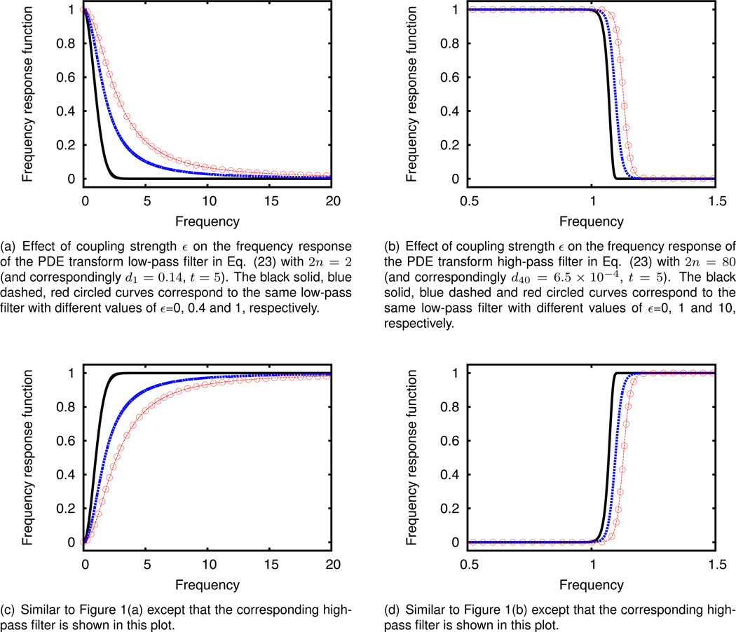
Obviously, Ĥ = 1 − L̂ is a high-pass filter. The effects of highest order 2n, propagation time t and coupling strength ε on the frequency response behavior of high-pass filter Ĥ is given in Figures 1 and 2. Qualitatively, the behavior of L̂ and Ĥ can be analyzed as . In particular, the impact of higher order, i.e., large 2m and 2n values, should be examined separately.
Figure 1.
Fourier analysis of the high-order PDE based low- and high-pass filters in Eqs. (21) and (23). Obviously, the time-frequency localization is controlled by parameter 2n, the highest order of the PDE transform. The effects of coupling strength ε (i.e. fidelity term) on the frequency responses L̂ and Ĥ are given. The values of the parameters in Eqs. (21) and (23) are given in the caption below each subfigures.
Figure 2.
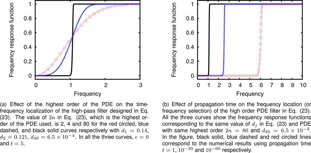
The control of the time-frequency localization by 2n and the frequency location (precision) by t of the high-order PDE high-pass filter in Eq. (23).
It is also interesting to investigate a band-pass filter given by the difference of solutions of two high-order PDEs. To this end, one can simply set ε = 0 and define
| (24) |
where we choose d2j >> d1j ~ 0 and t2 ≥ t1. Qualitatively, the behavior of B̂ can be analyzed as .
In Figures 1 and 2, Fourier analysis for the low-order PDE based low-pass filter in Eq. (21) and high-pass filter in Eq. (23) is given. We illustrate the control of the frequency localization by parameter 2n, the highest order of the PDE transform. The effects of coupling strength ε (i.e., fidelity term) on the frequency response behavior of the low-pass filter L̂ corresponding to the diffusion equation (with 2n = 2 being the highest order PDE) are given by the plots in Figure 1(a). The black curve shows the frequency response of the low-pass filter corresponding to the diffusion equation without fidelity term, i.e., ε = 0. The blue dashed and red circled curves correspond to the same low-pass filter with different values of ε=0.4 and 1, respectively. If the main purpose of the signal processing is to separate modes with close frequencies, a small ε value is preferred. On the other hand, as demonstrated in this paper, higher order PDEs provide much higher frequency localization and are more efficient in separating modes with closely adjacent frequencies. In Figure 1(b), the highest order of the PDE used is 2n = 80. The frequency responses approach to the ideal shape of a step function which provides higher precision in separating modes with closely adjacent frequencies.
The effect of ε, however, is different from that in the low order PDE case. The three curves of black, blue, and red color are frequency responses of the same low-pass filters with different values of ε = 0, 1, and 10. The large coupling strength (i.e., large value of ε) does not sacrifice the accuracy of mode decomposition as it does for the low order PDE; rather, the larger the value of ε, the higher shift of the dividing line of the mode frequency separation. In Figures 1(c) and 1(d), the symmetric plots of the high-pass filters are shown corresponding to the low-pass filters in Figures 1(a) and 1(b), respectively.
In Figure 2, the control of the time-frequency localization by 2n and the frequency selection by t of the highest order of the PDE, on the high-pass filter (23) are explored. The value of 2n in Figure 2(a) is equal to 2, 4 and 80 in the red circled, blue dashed, and black solid curves, respectively. As the order increases, the frequency response function becomes steeper and thus represents a better frequency localization, which is needed in the separation of closely adjacent frequency modes. In Figure 2(b) effect of propagation time is examined on the frequency response of the high order PDE filter in Eq. (23). All the three curves show the frequency response functions corresponding to different values of t with the same PDE. In the figure, black solid, blue dashed and red circled lines correspond to the numerical results using t = 1, 10−30 and 10−60, respectively. Therefore, one can gradually propagate the coupled high order PDEs in the PDE transform algorithm to systematically extract various modes. The longer propagation time of PDE transforms, the lower frequency of the decomposed mode. The PDE transform algorithm is truly robust and automatic in decomposing signal into series of functional modes or intrinsic modes.
III Numerical tests and validations
Having analyzed the frequency response of a linear PDE transform, we validate the ability of PDE transform to separate IMFs from signals, and demonstrate such an ability with applications to signals containing closely adjacent frequency modes which have been practically very challenging.
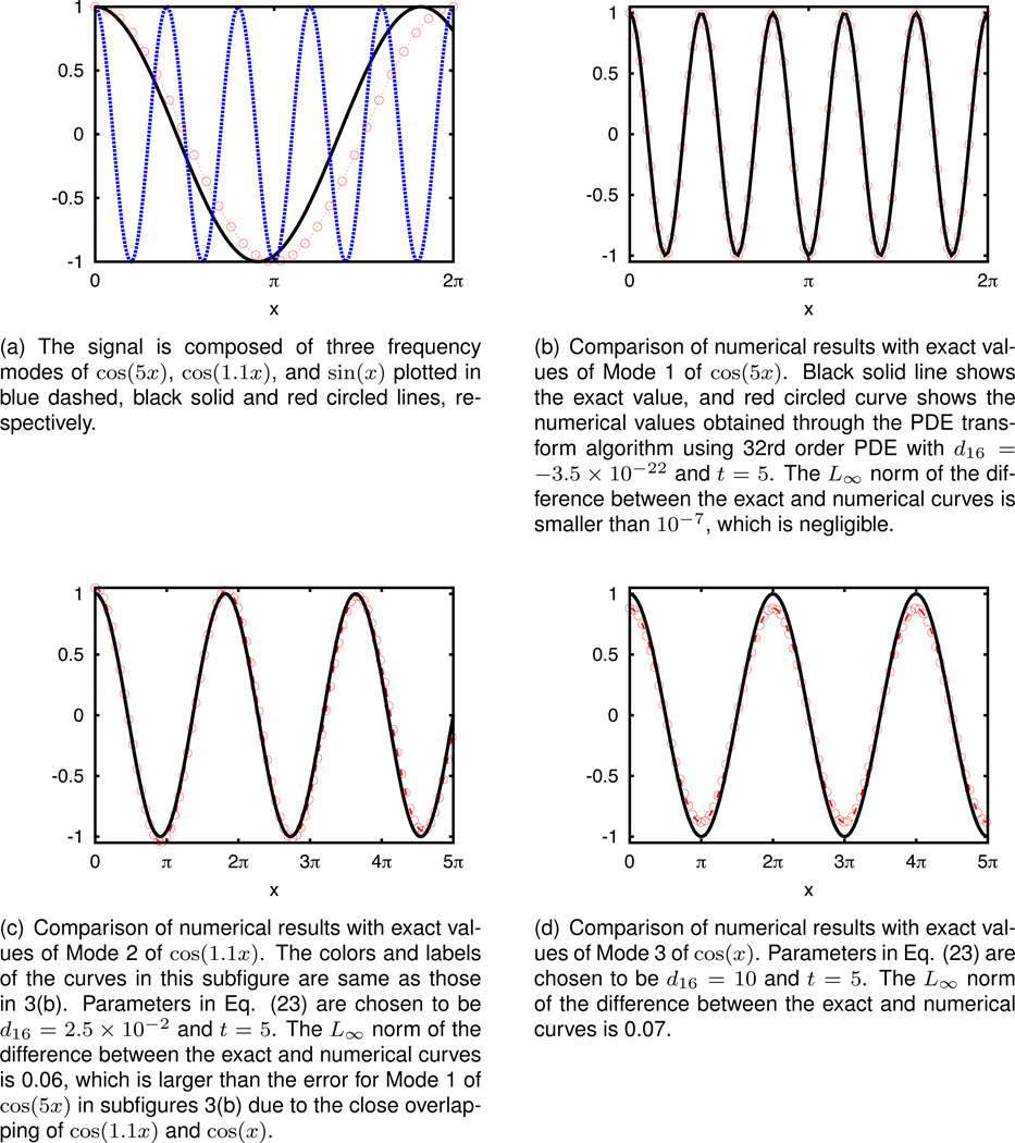
In Figure 3, the PDE transform is applied to the separation of the three modes (Figure 3(a)) from the signal cos(5x) + cos(1.1x) + cos(x). The highest order PDE used in the PDE transform is 2n = 32. The three modes are sequentially separated from the original signal using the same PDE transform algorithm with different values of propagation time t. This is a challenging case due to the extreme closeness of modes cos(1.1x) and cos(x). Numerical results for three modes are compared with exact values in Figures 3(b) through 3(d). In Figure 3(b), results for Mode 1, cos(5x), is shown. Black solid line shows the exact value, and red circles show the numerical values obtained by using the PDE transform algorithm with the 32nd order PDE. The L∞ norm of the difference between the exact and numerical curves is negligible (smaller than 10−6). Similarly in Figure 3(c), result of Mode 2, cos(1.1x), is shown. The L∞ norm of the difference between the exact and numerical curves is 0.06. In Figure 3(d), results of Mode 3, cos(x), is shown. The L∞ norms of the difference between the exact and numerical curves is 0.07 such that two closely adjacent modes cos(1.1x) and cos(x) are well separated. Additionally, higher order PDE can be easily applied to achieve even better accuracy as illustrated in Figure 4.
Figure 3.
Separation of the three modes from the signal cos(5x) + cos(1.1x) + cos(x) using the PDE transform algorithm with the PDE of the highest order of 2n = 32. The three modes are sequentially separated from the original signal using the same PDE transform algorithm with different propagation time t, respectively.
Figure 4.
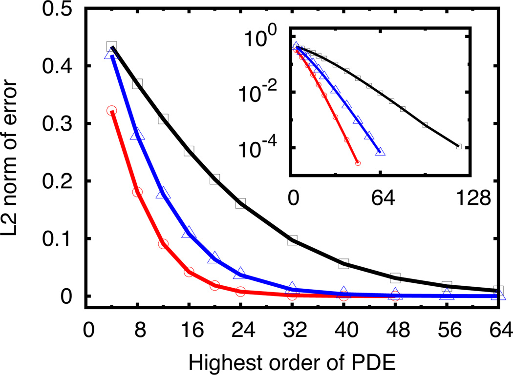
Extraction of higher frequency mode sin(mx) from the original signal sin(x) + sin(mx). In the main window of the figure, x-axis is the highest order of PDE employed in the PDE transform algorithm, and y-axis is the L2 norm error of the high frequency mode numerically extracted compared with the exact values of sin(mx). Three different signals of sin(x) + sin(1.1x), sin(x)+sin(1.2x) and sin(x)+sin(1.3x) are decomposed by the PDE transform algorithm, and their numerical results are shown by black square, blue triangle and red circled curves. The first signal of sin(x)+sin(1.1x) with closest overlapping modes requires much higher order of PDEs to be included in the PDE transform algorithm in order to achieve the same level of accuracy (or error) as for the other two signals. For the purpose of alternative viewing and better understanding, numerical errors are also plotted in log-scale as in the embedded smaller subfigure in the main window above. It is clearly observed that the PDE transform algorithm with higher order PDE achieves higher accuracy and better resolution in differentiating two modes with closely adjacent frequencies.
In Figure 4, convergence is checked with respect to the value of 2n, which is the highest order PDE used in the PDE transform. A series of signals are designed as composition of the lower frequency mode sin(x) with the higher frequency one sin(mx), where m varies from 1.3 to 1.1 in the figure. In the main window of the figure, x-axis is the highest order of PDE employed in the PDE transform algorithm, and y-axis is the L2 norm of the error of the high frequency mode numerically extracted compared with the exact values of sin(mx). Three different signals of sin(x) + sin(1.1x), sin(x) + sin(1.2x) and sin(x)+sin(1.3x) are decomposed by the PDE transform algorithm. The numerical results are shown by black square, blue triangle and red circled curves. The signal sin(x)+sin(1.1x) with two closest adjacent modes requires much higher order of PDEs to be included in the PDE transform algorithm in order to achieve the same level of accuracy (or error) as for the other two signals. For example, in order to achieve numerical accuracy with L2 error bounded below 0.1, a very high order PDE (2n=64) is required for mode decomposition of the signal with m = 1.1 compared to (roughly) 36th and 24th order PDEs needed for signals with m = 1.2 and m = 1.3, respectively. For better viewing and clearer quantitative comparison, numerical errors are also plotted in log-scale in the embedded small window in Figure 4. It is clearly observed that the PDE transform with higher order PDE achieves higher accuracy and better resolution in mode decomposition.
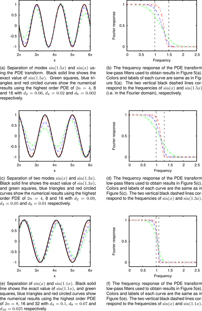
More detailed exploration of the convergence of the numerical results shown in Figure 4 is illustrated in Figure 5. The same PDE transform is used to decomposing three signals, sin(x) + sin(1.5x), sin(x) + sin(1.5x) and sin(x) + sin(1.5x) are shown in the 1st, 2nd and 3rd row in Figure 5, respectively. In the 1st row, the figure on the left shows the numerical results compared to the exact results for the higher frequency mode sin(1.5x) separated out from the signal using high-pass filter designed for the high order PDE transform algorithm. Exact results are shown by the black curve, while green squares, blue triangles and red circled curves show the numerical results using highest order PDE with 2n =4, 8 and 16, respectively. Similar results are shown in the 2nd row of Figure 5 where the PDE transform is applied to decompose signal sin(x)+sin(1.3x). In the 3rd row, due to the closeness of the two modes sin(x) and sin(1.1x), higher order PDEs are required to achieve accurate decomposition. In Figures 5(e) and 5(f), green squares, blue triangles and red circled curves show the numerical results using highest order PDE with 2n =8, 16 and 32, respectively. For all signals, it is clearly demonstrated that the PDE transform with larger value of n converges better to the exact results. In addition, the figures on the right of all the three rows in Figure 5 show the shape of the frequency responses for the corresponding low-pass filters (i.e. equivalently for the corresponding high-pass filters) designed by the PDE transform algorithm. The larger value n, the steeper the rising of frequency response functions. In the limit of n → ∞, the frequency response function would become a step function which ideally divide the frequency domain into high frequency and low frequency regions.
Figure 5.
Separation of the two modes sin(x) and sin(mx), where m ≈ 1, from the same signal. Convergence of the PDE transform algorithm with various highest order PDEs are studied. A higher order PDE transform is needed to differentiate modes with closer frequencies. Propagation time t = 5 in all the plots.
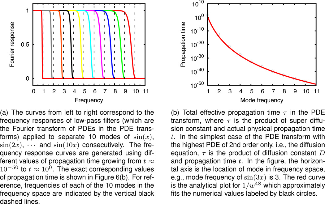
Lastly, in Figure 6, the effect of total propagation time t as in Eq. (23) on the frequency response functions is explored in details. The same PDE transform algorithm employing the same highest order PDE with 2n = 48 is applied to separate out all the modes from the signal sin(x) + sin(2x) + sin(3x) + sin(4x) + sin(5x) + sin(6x) + sin(7x) + sin(8x) + sin(9x) + sin(10x). The 10 modes are separated out, in the order of decreasing frequency peak, by varying propagation time t only. When the same set of PDEs composing the PDE transform algorithm are propagated by t = 4.3 × 10−48, highest frequency mode sin(10x) is decomposed; after another propagation time t = 9.4 × 10−46, next highest frequency mode sin(9x) is decomposed, etc. It is worthwhile to point out that, though the propagation time ranges from 10−50 to 1, no specific temporal discretization is needed in the current PDE scheme since the time integral is numerically calculated using one time step. In Figure 6(b), values of propagation time t are plotted as the function of the frequency peaks of the modes being decomposed. The numerical values of t (labeled by the black circles) fits well into the analytical estimation 1/w48 shown by the red solid curve, where the value of 48 corresponds to the value 2n = 48 of the highest order PDE used herein.
Figure 6.
Mode decomposition of the signal sin(x) + sin(2x) + sin(3x) + sin(4x) + sin(5x) + sin(6x) + sin(7x) + sin(8x) + sin(9x)+sin(10x) using the PDE transform algorithm including PDE terms up to 48th order with d24 = 1. The figure indicates that separation of lower frequency mode requires larger effective propagation time τ, or equivalently speaking larger effective diffusion constant.
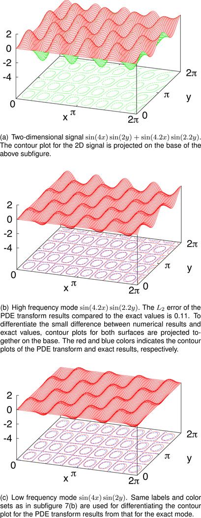
The PDE transform algorithm has been designed for the mode decomposition of arbitrary dimensional signals or images. In previous Figures, one-dimensional (1D) signals have been used for illustration and validation purposes. In Figure 7, a two-dimensional (2D) signal sin(4x) sin(2y) + sin(4.2x) sin(2.2y) is decomposed by the PDE transform algorithm into the two modes sin(4x) sin(2y) and sin(4.2x) sin(2.2y). A relatively low value of 2n = 16 for the highest order PDE is sufficient to achieve good enough numerical results of decomposed signal. L2 norm error is 0.1 compared to the amplitude 2.0. By increasing value 2n of the highest order PDEs employed in the PDE transform algorithm, similar convergence can be achieved as for 1D signals. The PDE transform algorithm has been designed to work naturally and equally efficient for arbitrarily dimensional signals and images.
Figure 7.
Mode decomposition of the signal sin(4x) sin(2y) + sin(4.2x) sin(2.2y) using the PDE transform algorithm including PDE terms up to 8th order. Results of two modes sin(4.2x) sin(2.2y) and sin(4x) sin(2y) are shown in subfigures 7(b) and 7(c), respectively.
IV Applications to biomedical and biological images
In this section, we apply the PDE transform algorithm to several different types of medical images for image denoising and enhancement.
IV.A Early cancer detection
In the initial period of the cancer development, the patient may not exhibit noticeable symptoms such that it would be too late even if they quickly pick up alerting messages when the cancer has developed for some time already. It is critical to detect cancer it its early state in order to provide a successful cure or surgery. Various medical imaging techniques have been developed to help diagnose and detect cancer. In addition to the hardware-type imaging techniques, image postprocessing can be applied to render a clearer image showing the important details of the cancer images. In this section, imaging techniques and processing are discussed with application to lung cancer and breast cancer.
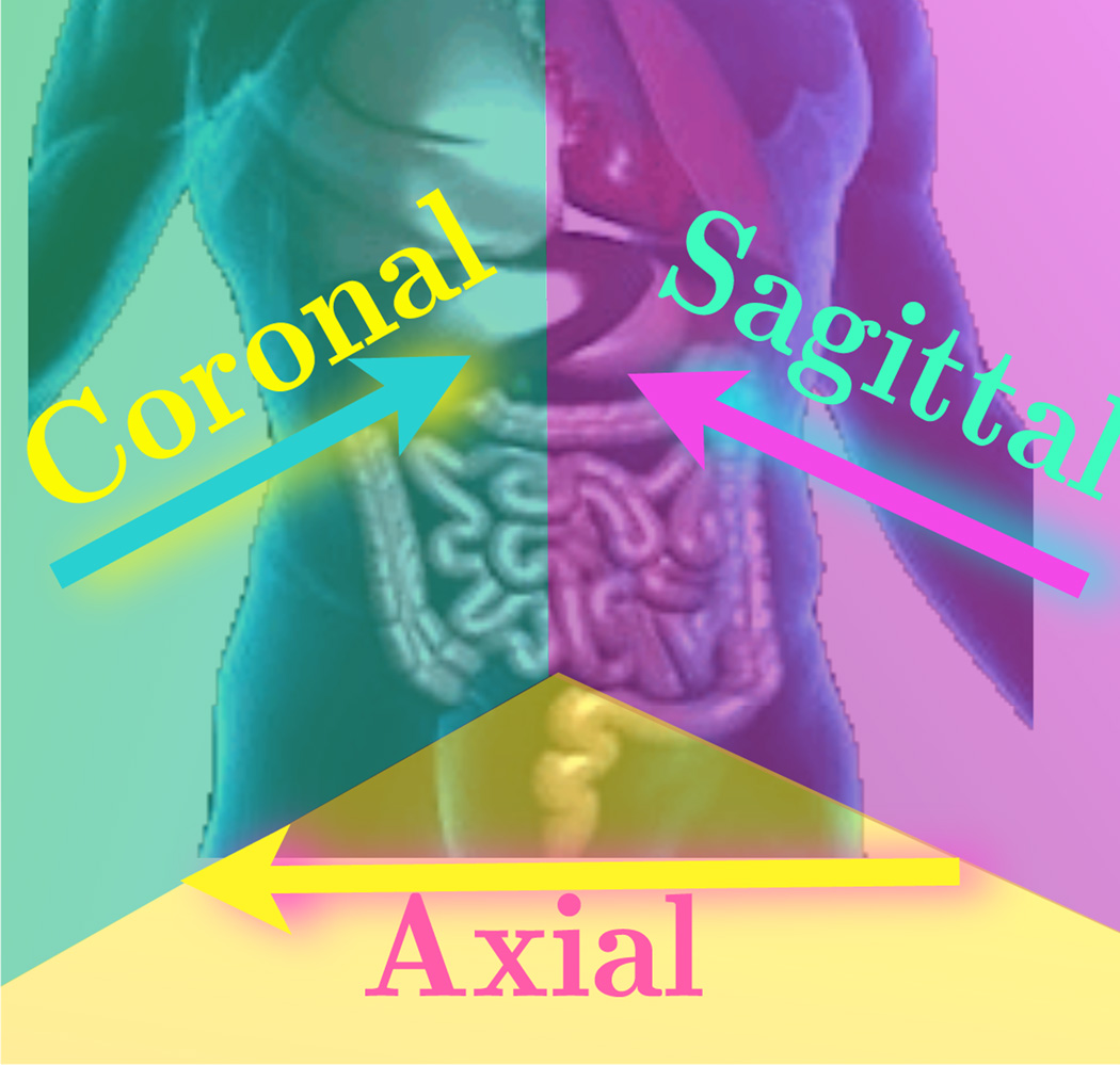
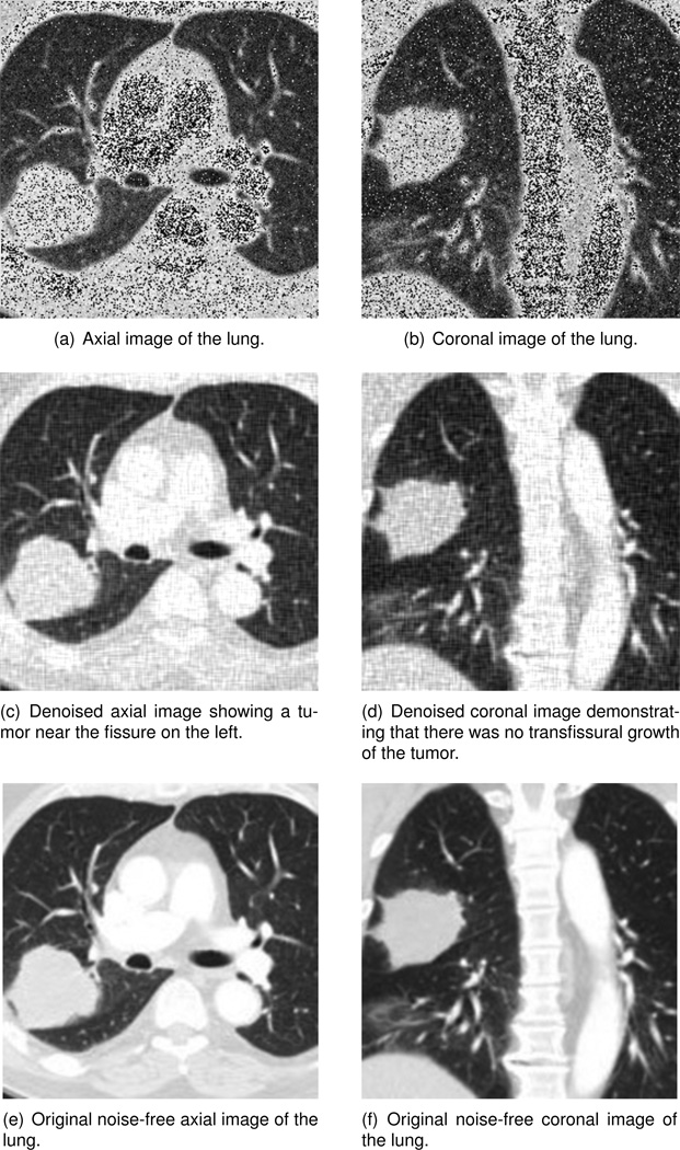
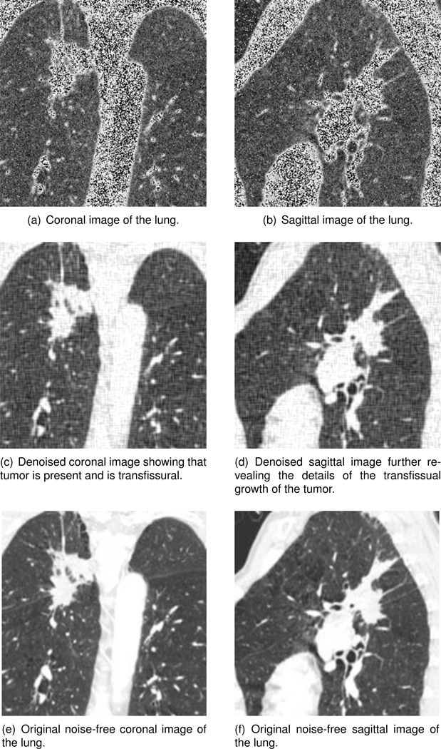
The general technique for early lung cancer is screening chest with X-ray or spiral computed tomography scan. Such a technique is useful for detecting the lung cancer in its more localized phase which implies it is more likely to be curable. One important goal of imaging and image processing is to decide whether the tumor is resectable and whether it should be a lobectomy or a pneumonectomy. Lobectomy means surgical excision of a lobe of the lung. On the other hand, a pneumonectomy is a surgical procedure to remove the whole lung. Clearly the lobectomy approach is a better and safer choice than pneumonectomy if the former is possible. The restriction for performing a lobectomy of the lung is that the surgery can not be performed on patients with lung cancers spreading to other parts of the tissue. Details from the medical images are therefore helpful in making the decision. In medical imaging or internal organs or brain, pictures are usually taken along one or many of the three planes (see Figure 8): axial plane which refers to the slice parallel to the feet of the patient, coronal plane which is the slice perpendicular to the feet and parallel to the shoulder line of the patient, and sagittal plane which is the vertical plane passing from front to rear and dividing the body into right and left sections. Images taken on the three planes together give three dimensional information of the internal organ of the human body. In Figures 9(e) and 9(f), images of the patient’s lung taken along the axial and coronal planes are shown respectively. To test the effect of the PDE transform algorithm, random (Gaussian-type) noise are added in Figures 9(a) and 9(b). The PDE transform algorithm with up to 4th order PDE is used to smooth and enhance the images, results of which are shown in 9(c) and 9(d). In the axial image 9(c), one can see the shape of tumor near the fissure on the left. However, this information alone is not enough for making decision whether the tumor is resectable and whether it should be a lobectomy or a pneumonectomy. The image in 9(d) taken along the coronal plane clearly shows there is no transfissural growth. As such, the tumor is localized and does not cross the fissure which divides the superior lobe from the middle lobe. Therefore lobectomy is a possibility. The lung of another patient is imaged along coronal and sagittal planes as shown in Figure 10. Similarly, white noise is added to the images and the PDE transform algorithm with up to 4th order PDE is performed to smooth the images. Comparing Figure 9(c) with 10(c), transfissural growth is observed in the latter case. The picture taken along the sagittal plane in Figure 10(d) further demonstrates that the tumor crosses the horizontal fissure of the lung. Therefore, lobectomy is not possible according to the images shown in these Figures.
Figure 8.
The axial plane is an imaginary plane that divides the body into superior and inferior parts. A coronal plane divides the body into back and front portions. A sagittal plane is a vertical plane which passes from front to rear dividing the body into right and left sections. The three planes are perpendicular to each others.
Figure 9.
PDE transform algorithm using up to 4th order PDE is used to denoise and enhance the images for lung diagnosis. The tumor is detected in the axial image, and the details shown in the coronal image demonstrates that there was no transfissural growth of the tumor such that lobectomy surgical excision of a lobe only is possible.
Figure 10.
PDE transform algorithm using up to 4th order PDE is used to denoise and enhance the images for lung diagnosis. The coronal image shows that there was transfissural growth of the tumor, and sagittal image reveals more details supporting the diagnosis that lobectomy surgical excision of a lobe only is not possible and pneumonectomy is a surgical procedure might be needed to remove the whole lung.
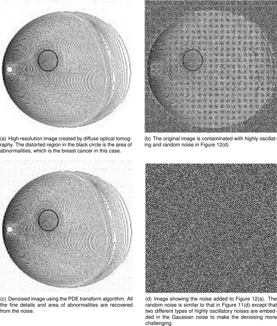
Detection of breast cancer is another important application of medical imaging and image processing. One of the widely used exams for early detection of breast cancer is mammogram, which take picture of breast with a safe, low-dose X-ray machine. Diffuse optical tomography (DOT) has recently been used to create high-resolution images from a scattering of infrared and visible light for the early detection of breast cancer. DOT is a three-dimensional method where photon density waves are launched from a source and then travel in a banana-shaped path due to multiple scattering, which is different from the straight paths followed by X-rays in mammogram. Compared to the use of X-rays in mammogram imaging, DOT is relatively less expensive, safer and more comfortable. However, the photon density waves used in DOT are more difficult to track because of the scattering and absorption. Image processing is usually performed to remove noise and enhance image quality. In Figure 12(a), a high resolution image is shown created by the DOT technology. The distorted region in the black circle in the image indicates the area of abnormalities associated with the breast cancer. Image shown in Figure 12(b) contains combination of two types of noises: highly oscillatory random noises (with up to 200 oscillations in each direction of the 256×256-pixel image and with random amplitude in each oscillation) and Gaussian-type random noise with standard deviation equal to 30 (see Figure 12(d)). The fine lines of image are therefore distorted and contaminated. In Figure 12(c), an enhanced image is generated from the Figure 12(b) by applying the PDE transform algorithm using up to 4th order PDE. The fine details are well recovered. Such image enhancement can be combined with other mathematical models in development by other groups to make the DOT a better imaging techniques for detecting smaller breast cancer with lower cost and higher safety and reliability.
Figure 12.
Diffuse optical tomography is used to create extremely high-resolution images from a scattering of infrared and visible light. Such technology can be used for the early detection of breast cancer. As light travels from the source, once it hits the black circle where the tumor is located, the lightwaves become distorted. One practical challenge is that the high resolution imaging is subject to noises, especially highly oscillatory noise which would distort the fine details in the image. The PDE transform can be used to smooth the image and is particularly good for removing high frequency noise and/or oscillatory noises.
IV.B Optical images from retinal functioning imager
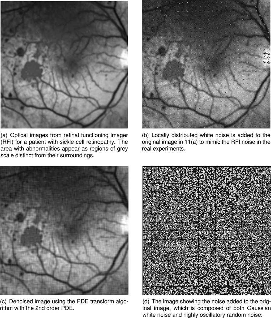
Besides the important biological function of vision, eyes are also helpful for the diagnosis of diseases such as diabetes as well as for the assessment and identification of various neurological effects. A number of technological progresses has advanced the retinal imaging for research and clinical applications, e.g. Many imaging techniques including retinal function imager (RFI), positron emission tomography (PET) and functional magnetic resonance imaging (fMRI) have been developed to provide high resolution images. In particular, RFI is an adaptive noninvasive approach to study the single red blood cells moving through capillaries26,31 and it enables direct visualization of retinal blood dynamics without the injection of contrast agents. The motion of individual red blood cells and blood cell clusters can be revealed with much clarity which is important towards the quantitative detection of abnormal blood flow velocity in capillaries and arterioles. Like many other medical imaging techniques, poor signal-to-noise ratio in in-vivo applications is always a concern. Various post image processing techniques are generally applied to render enhanced images. In Figure 11, qualitative oximetry with the RFI is applied to detect the perfusion deficits and abnormalities in a patient with sickle cell retinopathy. The area with abnormalities appear as regions of grey scale distinct from their surroundings. Figure 11(a) shows a high resolution image with good resolution. In Figure 11(b), noise is added which is composed of both a highly oscillatory noise (with up to 30 oscillations in each direction of the 256×256-pixel image) with random amplitudes and Gaussian-type random noise (with standard deviation equal to 30). The PDE transform algorithm using up to 4th order PDE is applied for denoising the image. Result is shown in Figure 11(c). Such image enhancement technique would be useful in further improving the image quality of high resolution RFI.
Figure 11.
Using qualitative oximetry with optical images from RFI, perfusion deficits and abnormalities in a patient with sickle cell retinopathy is detected. The PDE transform algorithm using up to 4th order PDE is used to denoise and enhance the RFI images.
IV.C Electron microscope photography of neuron systems
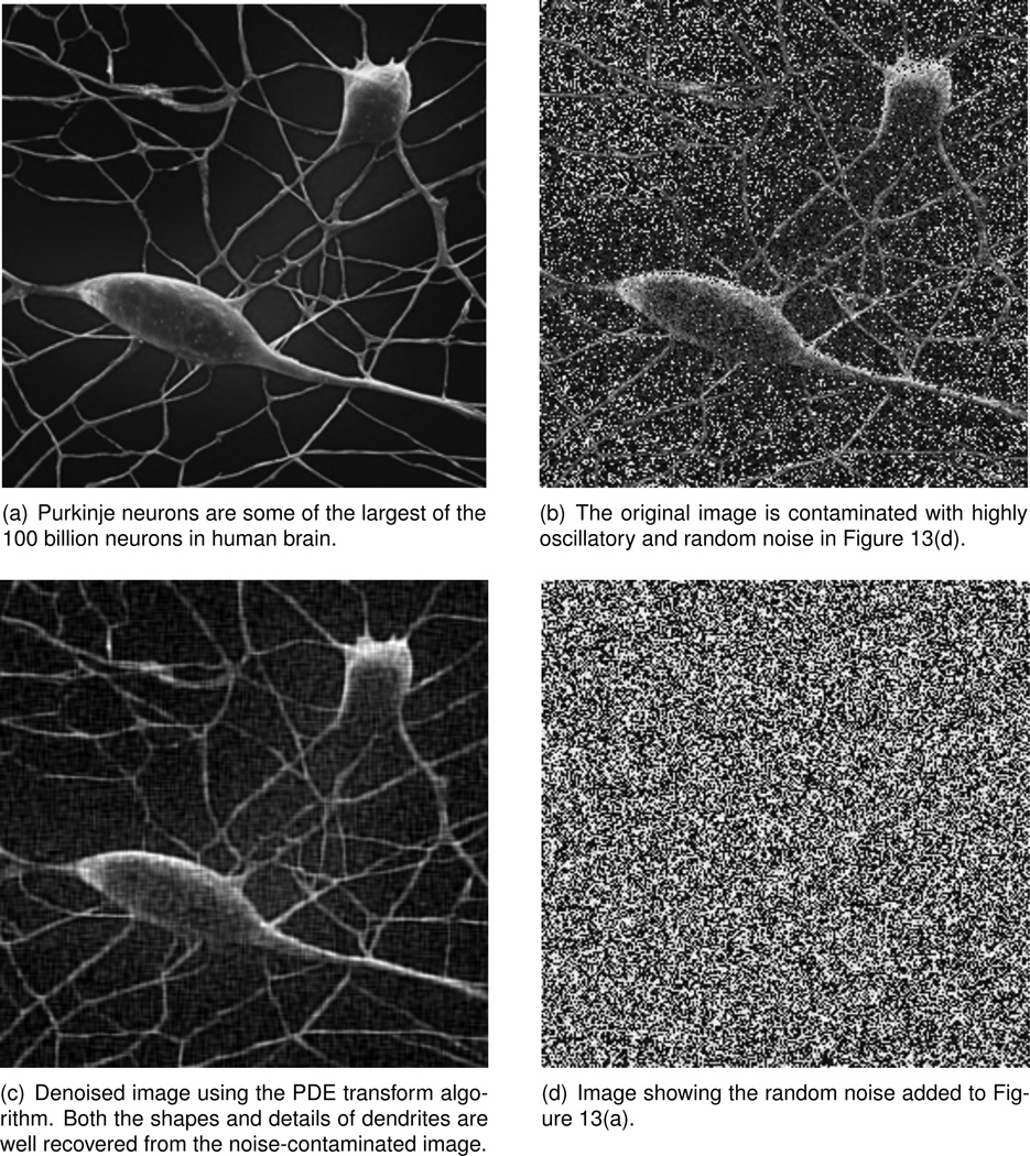
With an intricately elaborate dendritic arbor, Purkinje neurons are characterized by a large number of dendritic spines. Purkinje neurons are some of the largest of the 100 billion neurons in human brain. Neuron cells are the masters of motor coordination in the cerebellar cortex. These large dendritic arbors form nearly two-dimensional layers through which parallel fibers from the deeper-layers pass. Toxic exposure to such as alcohol and lithium and various immune or neurodegenerative diseases such as autism and Alzheimer’s disease can negatively affect human Purkinje cells and their shape and structure. Therefore, a clear visualization of the detailed shape of Purkinje neurons would be useful in the study and diagnosis of various diseases. In Figure 13, electron microscope photography of Purkinje neurons is shown. Electron microscope is a type of microscope that uses a particle beam of electrons to illuminate the sample and to generate a magnified image. Electron microscopes usually have a greater resolving power than a light-powered optical microscope due to the much smaller wavelength of electrons. Using electron microscope imaging technique, the details of vast amount of dendrites on the neuron cells. Noise removal using image processing can further provide a better quality image. The PDE transform using up to 4th order PDE is used to denoise the image 13(b) to generate a better resolved one in 13(c) in which the details of cell structure and geometry of the dendrites are better rendered compared to the original high resolution picture 13(a).
Figure 13.
Electron microscope photography of Purkinje neurons showing the details of vast amount of dendrites on the neuron cells. The PDE transform using up to 4th order PDE is used to denoise the image and enhance the details of cell structure and geometry details of the dendrites.
V Concluding remarks
Geometric partial differential equations (PDEs) are of tremendous importance in signal and image processing, data analysis and surface construction. Mode decomposition is an elementary process in a variety of signal/image processing tasks. However, despite the great progresses made in geometric PDEs accompanying the broad interests in the past two decades, the use of geometric PDEs for mode decomposition was not realized until a recent advance in the field. The resulting models, called PDE transform, has been introduced in our earlier work56 based on arbitrarily high order nonlinear PDE introduced by Wei59 and PDE based image edge operator introduced by Wei and Jia.61 The present work introduces the variational formulation, provides the Fourier analysis and carries out the biomedical and biological applications of the PDE transform.
In the variational formulation of PDE transform, we construct a total energy functional consisting of two image functions and two sets of geometric operators. Due to the dynamical coupling of two operators, the relative signs of two operators are different, which contributes to the energy disparity. The dynamical coupling of two image functions reduces the energy disparity. The energy minimization by using the Euler-Lagrange equation and the introduction of artificial propagation time by the steepest descent algorithm leads to a system of two coupled nonlinear PDE transforms. As discussed in our earlier work,59 these two equations have to evolve at dramatically different time scales to generate sufficient disparity in the two image functions. Their difference corresponds to the desirable intrinsic mode functions when appropriate model parameters and initial values are provided. To aid the parameter selection, we carried out detailed Fourier analysis on a prototype linear PDE transform, which admits an analytical solution in the Fourier domain. As such, we analyze the filter properties of arbitrarily high order PDE transforms. This analysis provides a guidance for the parameter selection of the proposed PDE transforms. For instance, the order of the highest PDE can be selected to control the frequency localization, while the propagation time or the amplitude of diffusion coefficients of the PDE transform can be adjusted to control the frequency location or precision. Many challenging test examples are explored to validate the proposed PDE transforms for decomposing intrinsic mode functions. We demonstrate usefulness of the proposed PDE transforms by biomedical and biological applications. Image denoising, enhancement and restoration are considered in the present work for early lung cancer detection, optical image, diffuse optical tomography, and electron microscope photography. Numerical experiments indicate that the proposed PDE transform works well.
Acknowledgments
This work was supported in part by NSF grants CCF-0936830 and DMS-1043034; NIH grant R01GM-090208; MSU Competitive Discretionary Funding Program grant 91-4600.
Literature cited
- 1.Barbu T, Barbu V, Biga V, Coca D. A PDE variational approach to image denoising and restoration. Nonlinear Analysis Real World Applications. 2009;10(3):1351–1361. [Google Scholar]
- 2.Bates PW, Chen Z, Sun YH, Wei GW, Zhao S. Geometric and potential driving formation and evolution of biomolecular surfaces. Journal of Mathematical Biology. 2009;59(2):193–231. doi: 10.1007/s00285-008-0226-7. [DOI] [PubMed] [Google Scholar]
- 3.Bates PW, Wei GW, Zhao S. Minimal molecular surfaces and their applications. Journal of Computational Chemistry. 2008;29(3):380–391. doi: 10.1002/jcc.20796. [DOI] [PubMed] [Google Scholar]
- 4.Bertalmio M. Strong-continuation, contrast-invariant inpainting with a third-order optimal PDE. IEEE Transactions on Image Processing. 2006;15(7):1934–1938. doi: 10.1109/tip.2006.877067. [DOI] [PubMed] [Google Scholar]
- 5.Bertozzi AL, Greer JB. Low-curvature image simplifiers: Global regularity of smooth solutions and laplacian limiting schemes. Communications on Pure and Applied Mathematics. 2004;57(6):764–790. [Google Scholar]
- 6.Caselles V, Kimmel R, Sapiro G. Geodesic active contours. International Journal of Computer Vision. 1997;22(1):61–79. [Google Scholar]
- 7.Caselles V, Morel JM, Sapiro G, Tannenbaum A. Introduction to the special issue on partial differential equations and geometry-driven diffusion in image processing and analysis. IEEE Transactions on Image Processing. 1998;7(3):269–273. doi: 10.1109/TIP.1998.661176. [DOI] [PubMed] [Google Scholar]
- 8.Catte F, Lions PL, Morel JM, Coll T. Image selective smoothing and edge-detection by nonlinear diffusion. SIAM Journal on Numerical Analysis. 1992;29(1):182–193. [Google Scholar]
- 9.Chambolle A, Lions PL. Image recovery via total variation minimization and related problems. Numerische Mathematik. 1997;76(2):167–188. [Google Scholar]
- 10.Chan T, Kang S, Shen J. Euler’s elastica and curvature-based inpainting. SIAM Journal on Applied Mathematics. 2002:564–592. [Google Scholar]
- 11.Chan T, Marquina A, Mulet P. High-order total variation-based image restoration. SIAM Journal on Scientific Computing. 2000;22(2):503–516. [Google Scholar]
- 12.Chan T, Vese L. Active contours without edges. IEEE Transactions on Image Processing. 2001;10(2):266–277. doi: 10.1109/83.902291. [DOI] [PubMed] [Google Scholar]
- 13.Chan Y. Wavelet basics. Springer: 1995. [Google Scholar]
- 14.Chen D, Wei GW. Modeling and simulation of nano-electronic devices. Journal of Computational Physics. 2010;229:4431–4460. doi: 10.1016/j.jcp.2010.02.002. [DOI] [PMC free article] [PubMed] [Google Scholar]
- 15.Chen Z, Baker NA, Wei GW. Differential geometry based solvation models I: Eulerian formulation. Journal of Computational Physics. 2010;229:8231–8258. doi: 10.1016/j.jcp.2010.06.036. [DOI] [PMC free article] [PubMed] [Google Scholar]
- 16.Chen Z, Baker NA, Wei GW. Differential geometry based solvation models II: Lagrangian formulation. Journal of Mathematical Biololgy. 2010 doi: 10.1007/s00285-011-0402-z. accepted. [DOI] [PMC free article] [PubMed] [Google Scholar]
- 17.Daubechies I. Ten Lectures on Wavelets. Philadelphia: SIAM; 1992. [Google Scholar]
- 18.Didas S, Weickert J, Burgeth B. Properties of higher order nonlinear diffusion filtering. Journal of Mathematical Imaging and Vision. 2009;35(3):208–226. [Google Scholar]
- 19.Dugatkin D, Zhou HM, Chan TF, Effros M. Lagrangian optimization of a group testing for ENO wavelets algorithm. Proceedings to the 2002 Conference on Information Sciences and Systems; Princeton University; New Jersey. 2002. pp. 20–22. [Google Scholar]
- 20.Farge M. Wavelet transforms and their applications to turbulence. Annual Review of Fluid Mechanics. 1992;24:395–457. [Google Scholar]
- 21.Gilboa G, Sochen N, Zeevi YY. Forward-and-backward diffusion processes for adaptive image enhancement and denoising. IEEE Transactions on Image Processing. 2002;11(7):689–703. doi: 10.1109/TIP.2002.800883. [DOI] [PubMed] [Google Scholar]
- 22.Gilboa G, Sochen N, Zeevi YY. Image sharpening by flows based on triple well potentials. Journal of Mathematical Imaging and Vision. 2004;20(1–2):121–131. [Google Scholar]
- 23.Greer JB, Bertozzi AL. H-1 solutions of a class of fourth order nonlinear equations for image processing. Discrete and Continuous Dynamical Systems. 2004;10(1–2):349–366. [Google Scholar]
- 24.Greer JB, Bertozzi AL. Traveling wave solutions of fourth order PDEs for image processing. SIAM Journal on Mathematical Analysis. 2004;36(1):38–68. [Google Scholar]
- 25.Grimm V, Henn S, Witsch K. A higher-order PDE-based image registration approach. Numerical Linear Algebra with Applications. 2006;13(5):399–417. [Google Scholar]
- 26.Grinvald A, Lieke E, Frostig R, Gilbert C, Wiesel T. Functional architecture of cortex revealed by optical imaging of intrinsic signals. Nature. 1986;324:361–364. doi: 10.1038/324361a0. [DOI] [PubMed] [Google Scholar]
- 27.Gu Y, Wei GW. Conjugate filter approach for shock capturing. Communications in Numerical Methods in Engineering. 2003;19(2):99–110. [Google Scholar]
- 28.Guan S, Lai C, Wei G. A wavelet method for the characterization of spatiotemporal patterns. Physica D: Nonlinear Phenomena. 2002;163(1–2):49–79. [Google Scholar]
- 29.Hou ZJ, Wei GW. A new approach to edge detection. Pattern Recognition. 2002;35(7):1559–1570. [Google Scholar]
- 30.Huang NE, Long SR, Shen Z. The mechanism for frequency downshift in nonlinear wave evolution. Advances in Applied Mechanics. 1996;Vol 32(32):59. [Google Scholar]
- 31.Izhaky D, Nelson D, Burgansky-Eliash Z, Grinvald A. Functional imaging using the retinal function imager: Direct imaging of blood velocity, achieving fluorescein angiography-like images without any contrast agent, qualitative oximetry, and functional metabolic signals. Japanese Journal of Ophthalmology. 2009;53(4):345–351. doi: 10.1007/s10384-009-0689-0. [DOI] [PubMed] [Google Scholar]
- 32.Jain AK. Partial-differential equations and finite-difference methods in image-processing .1. image representation. Journal of Optimization Theory and Applications. 1977;23(1):65–91. [Google Scholar]
- 33.Jin JH, Shi JJ. Feature-preserving data compression of stamping tonnage information using wavelets. Technometrics. 1999;41(4):327–339. [Google Scholar]
- 34.Jin ZM, Yang XP. Strong solutions for the generalized Perona-Malik equation for image restoration. Nonlinear Analysis-Theory Methods and Applications. 2010;73(4):1077–1084. [Google Scholar]
- 35.Karras DA, Mertzios GB. New PDE-based methods for image enhancement using SOM and bayesian inference in various discretization schemes. Measurement Science Technology. 2009;20(10):8. [Google Scholar]
- 36.Liang HL, Lin QH, Chen JDZ. Application of the empirical mode decomposition to the analysis of esophageal manometric data in gastroesophageal reflux disease. IEEE Transactions on Biomedical Engineering. 2005;52(10):1692–1701. doi: 10.1109/TBME.2005.855719. [DOI] [PubMed] [Google Scholar]
- 37.Lin L, Wang Y, Zhou H. Iterative filtering as an alternative algorithm for empirical mode decomposition. Advances in Adaptive Data Analysis. 2009;1(4):543–560. [Google Scholar]
- 38.Lysaker M, Lundervold A, Tai XC. Noise removal using fourth-order partial differential equation with application to medical magnetic resonance images in space and time. IEEE Transactions on Image Processing. 2003;12(12):1579–1590. doi: 10.1109/TIP.2003.819229. [DOI] [PubMed] [Google Scholar]
- 39.Mallat S. A Wavelet tour of signal processing. Academic Press; 1999. [Google Scholar]
- 40.Meyer FG, Coifman RR. Brushlets: A tool for directional image analysis and image compression. Applied and Computational Harmonic Analysis. 1997;4(2):147–187. [Google Scholar]
- 41.Nitzberg M, Shiota T. Nonlinear image filtering with edge and corner enhancement. IEEE Transactions on Pattern Analysis and Machine Intelligence. 1992;14(8):826–833. [Google Scholar]
- 42.Oppenheim AV, Schafer RW. Digital Signal Process. Englewood Cliffs, NJ: Prentice-Hall; 1989. [Google Scholar]
- 43.Osher S, Sethian J. Fronts propagating with curvature-dependent speed: algorithms based on Hamilton-Jacobi formulations. Journal of computational physics. 1988;79(1):12–49. [Google Scholar]
- 44.Perona P, Malik J. Scale-space and edge-detection using anisotropic diffusion. IEEE Transactions on Pattern Analysis and Machine Intelligence. 1990;12(7):629–639. [Google Scholar]
- 45.Pesenson M, Roby W, McCollum B. Multiscale astronomical image processing based on nonlinear partial differential equations. Astrophysical Journal. 2008;683(1):566–576. [Google Scholar]
- 46.Rudin LI, Osher S, Fatemi E. Nonlinear total variation based noise removal algorithms. Physica D. 1992;60(1–4):259–268. [Google Scholar]
- 47.Sazonov I, Yeo SY, Bevan RLT, Xie XH, van Loon R, Nithiarasu P. Modelling pipeline for subject-specific arterial blood flow — a review. International Journal for Numerical Methods in Biomedical Engineering. 2011:1–46. in press. [Google Scholar]
- 48.Sethian J. Evolution, implementation, and application of level set and fast marching methods for advancing fronts. Journal of Computational Physics. 2001;169(2):503–555. [Google Scholar]
- 49.Shih Y, Rei C, Wang H. A novel PDE based image restoration: Convection-diffusion equation for image denoising. Journal of Computational and Applied Mathematics. 2009;231(2):771–779. [Google Scholar]
- 50.Soltanianzadeh H, Windham JP, Yagle AE. A multidimensional nonlinear edge-preserving filter for magnetic-resonance image-restoration. IEEE Transactions on Image Processing. 1995;4(2):147–161. doi: 10.1109/83.342189. [DOI] [PubMed] [Google Scholar]
- 51.Spedding GR, Browand FK, Huang NE, Long SR. A 2-d complex wavelet analysis of an unsteady wind-generated surface-wave field. Dynamics of Atmospheres and Oceans. 1993;20(1–2):55–77. [Google Scholar]
- 52.Sun YH, Wu PR, Wei G, Wang G. Evolution-operator-based single-step method for image processing. International Journal of Biomedical Imaging. 2006;83847:1. doi: 10.1155/IJBI/2006/83847. [DOI] [PMC free article] [PubMed] [Google Scholar]
- 53.Sun YH, Zhou YC, Li SG, Wei GW. A windowed Fourier pseudospectral method for hyperbolic conservation laws. Journal of Computational Physics. 2006;214(2):466–490. [Google Scholar]
- 54.Tasdizen T, Whitaker R, Burchard P, Osher S. Geometric surface processing via normal maps. Acm Transactions on Graphics. 2003;22(4):1012–1033. [Google Scholar]
- 55.Titchmarsh EC. Introduction to the theory of Fourier integrals. Oxford University Press; 1948. [Google Scholar]
- 56.Wang Y, Wei G, Yang S. Mode decomposition evolution equations. 2010 doi: 10.1007/s10915-011-9509-z. submitted. [DOI] [PMC free article] [PubMed] [Google Scholar]
- 57.Wang Y, Wei G, Yang S. Iterative filtering decomposition based on local spectral evolution kernel. Journal of Scientific Computing. 2011 doi: 10.1007/s10915-011-9496-0. accepted. [DOI] [PMC free article] [PubMed] [Google Scholar]
- 58.Wei G. Differential geometry based multiscale models. Bulletin of Mathematical Biology. 2010;27:1562–1622. doi: 10.1007/s11538-010-9511-x. [DOI] [PMC free article] [PubMed] [Google Scholar]
- 59.Wei GW. Generalized Perona-Malik equation for image restoration. IEEE Signal Processing Letters. 1999;6(7):165–167. [Google Scholar]
- 60.Wei GW. Wavelets generated by using discrete singular convolution kernels. Journal of Physics A: Mathematical and General. 2000;33:8577–8596. [Google Scholar]
- 61.Wei GW, Jia YQ. Synchronization-based image edge detection. Europhysics Letters. 2002;59(6):814–819. [Google Scholar]
- 62.Witelski TP, Bowen M. Adi schemes for higher-order nonlinear diffusion equations. Applied Numerical Mathematics. 2003;45(2–3):331–351. [Google Scholar]
- 63.Witkin A. Scale-space filtering: A new approach to multi-scale description. Proceedings of IEEE International Conference on Acoustic Speech Signal Processing; Institute of Electrical and Electronics Engineers; 1984. pp. 150–153. [Google Scholar]
- 64.Wu JY, Ruan QQ, An GY. Exemplar-based image completion model employing PDE corrections. Informatica. 2010;21(2):259–276. [Google Scholar]
- 65.Xu M, Zhou SL. Existence and uniqueness of weak solutions for a fourth-order nonlinear parabolic equation. Journal of Mathematical Analysis and Applications. 2007;325(1):636–654. [Google Scholar]
- 66.Yang S, Coe J, Kaduk B, Martínez T. An optimal spawning algorithm for adaptive basis set expansion in nonadiabatic dynamics. Journal of Chemical Physics. 2009;130 doi: 10.1063/1.3103930. 134113. [DOI] [PubMed] [Google Scholar]
- 67.Yezzi A, et al. A fully global approach to image segmentation via coupled curve evolution equations. Journal of Visual Communication and Image Representation. 2002;13(1–2):195–216. [Google Scholar]
- 68.You Y, Kaveh M. Fourth-order partial differential equations for noise removal. IEEE Transactions on Image Processing. 2002;9(10):1723–1730. doi: 10.1109/83.869184. [DOI] [PubMed] [Google Scholar]
- 69.Zhao S, Wei GW. Jump process analysis for the trend estimation of time series. Computational Statistics and Data Analysis. 2003;42:219–241. [Google Scholar]


