Discrimination of the spectral density of multitone complexes

Abstract

Spectral density (D), defined as the number of partials comprising a sound divided by its bandwidth, has been suggested as cue for the identification of the size and shape of sound sources. Few data are available, however, on the ability of listeners to discriminate differences in spectral density. In a cue-comparison, forced-choice procedure with feedback, three highly practiced listeners discriminated differences in the spectral density of multitone complexes varying in bandwidth (W = 500–1500 Hz), center frequency (f_c = 500–2000 Hz), and number of tones (N = 6–31). To reduce extraneous cues for discrimination, the overall level of the complexes was roved, and the frequencies were drawn at random uniformly over a fixed bandwidth and center frequency for each presentation. Psychometric functions were obtained relating percent correct discrimination to ΔD in each condition. For D < 0.02 Hz⁻¹, the steepness of the functions remained constant across conditions, but for D > 0.02 Hz⁻¹, they increased with D. The increase, moreover, was accompanied by a reduction in the upper asymptote of the functions. The data were well fit by a model in which spectral density discrimination is determined by the frequency separation of components on an equivalent rectangular bandwidth scale, yielding a roughly constant Weber fraction of ΔD/D = 0.3.

INTRODUCTION

A fundamental goal of psychoacoustic research is to determine the extent of a listener’s ability to identify properties of objects and events from the sounds they produce (reviewed by Lutfi, 2008; McAdams, 1993; Bregman, 1990). Relevant acoustic information for various source properties (material, size, shape, and the like) has been identified by means of physical-acoustic analyses (e.g., Wildes and Richards, 1988; Kunkler-Peck and Turvey, 2000; Lutfi, 2001; Lutfi and Oh, 1997; McAdams et al., 2004) and is regularly implicated as the basis for listener judgments in studies. Yet little is known regarding the limits of listeners’ basic sensitivity to this information (cf. Lutfi and Stoelinga, 2009). The present study measured limits of sensitivity for one source of acoustic information deemed relevant for auditory identification of object size and shape (Lutfi, 2008)—that of spectral density.

Spectral density is a measure of the concentration of partials in the emitted sound over their frequency range. It is technically defined as

$$D=\frac{N}{f_{\max }-f_{\min }},$$ (1)

where N is the number of partials and f_min and f_max are the lowest and highest frequency partials. To see how D might serve as a cue to object size and shape, consider the sound emitted by a simply supported rectangular plate struck with a mallet (a popular sound source used in studies). The modal frequencies of the simply supported rectangular plate are well known (see, for instance, Rossing and Fletcher, 1999, p. 75). They are

$$f_{\mathit{mn}}=0.453c_{l}h[{\left(\frac{m+1}{L_x}\right)}^2+{\left(\frac{n+1}{L_y}\right)}^2],$$ (2)

where h is the thickness of the plate, L_x and L_y are the length and width of the plate, c_l is the velocity of longitudinal waves in the plate, and m and n are non-negative integers indicating the different modes of vibration. Now consider two plates that are equal in all respects except that for one, the length L_x is twice as large. For the larger plate, the odd values of m will yield the same frequencies as the smaller plate for certain even values of m. However, for the larger plate the even values of m will result in an extra component in between the components of the smaller plate. The larger plate will, thus, have a higher spectral density. The same principle applies to plates of other shapes where the modal frequencies are determined numerically, and to the distinction between plates and bars (Rajalingham et al., 1995; Lutfi, 2008).

Few studies to date have examined the ability of listeners to discriminate changes in spectral density despite its relevance for determining object size and shape. Thurlow and Rawlings (1959) conducted an early relevant study in which listeners were presented tone complexes consisting of one, two, or three components and were asked to judge the number of different tones in each complex. The results can only be taken as a crude measure of spectral density discrimination as bandwidth was confounded with number of components in the study and no feedback was provided to listeners. Notwithstanding, performance in judging the number of components was quite poor. There was also no evidence of any improvement in performance with increasing frequency separation among the tones.

Neff and Green (1987) also measured the ability of listeners to discriminate the number of components of multi-tone complexes but in a task somewhat closer to what could be called spectral density discrimination. In the two-interval, forced-choice procedure, listeners judged which of the two intervals contained the complex with the greater number of tones. The frequencies of the tones were selected at random uniformly over a fixed range of 0–5000 Hz, and feedback was given after each trial. Neff and Green found that discrimination of number of components N behaved according to Weber’s law. For values of N ranging from 1 to 100, performance was found to be constant for a constant Weber fraction of ΔN/N = 0.5.

Hartmann et al. (1986) measured spectral density discrimination also using a two-interval forced-choice task like that of Neff and Green. Listeners were presented two sounds in random order; one consisted of 60 frequency components, the other between 3 and 25 components. The frequency bandwidth was divided into evenly sized bins, and one component was positioned randomly within each bin. The listener’s task was to choose the sound having the larger number of components. Feedback was given only during training runs, which lasted until the subjects reported they had learned the task. Hartmann et al. concluded from their results that, except for large bandwidths, a constant bandwidth leads to constant performance as the center frequency of the band varies. They also presented a model suggesting that listeners could use power fluctuations in the sounds as cue for discriminating density.

The data from the studies of Neff and Green (1987) and Hartmann et al. (1986) represent the best data available to date regarding the ability of listeners to discriminate spectral density. Yet upon reexamination, the outcomes of these studies appear to be somewhat at odds. The bandwidth of signals and N are two parameters that vary independently to influence spectral density. Performance cannot, therefore, depend only on N and only on W at the same time. The apparent discrepancies in results can be attributed to differences in the procedures used in these studies. To begin, the procedure of Hartmann et al. for randomizing frequencies maintained a more nearly constant bandwidth for individual signals compared to the procedure used by Neff and Green. Hartmann et al. measured over a range of different bandwidths and center frequencies but for only one value of N (N = 60), whereas Neff and Green measured only over a range of values of N but for only one bandwidth. Also unlike Neff and Green, Hartmann et al. did not provide feedback to listeners on experimental trials and so may not have measured the best performance of listeners. Finally because of the differences in the number of tones and bandwidths selected for study, Hartmann et al. measured performance at very high levels of spectral density while Neff and Green measured performance at much lower levels. Any of these differences could easily have been responsible for the difference in results.

The present study was undertaken to further evaluate the factors affecting spectral density discrimination in an effort to better understand the apparent discrepancy in the outcomes of these studies. To this end, complete psychometric functions were obtained at both high and low spectral densities by varying the bandwidth, center frequency, and number of components in complexes. Feedback was presented on all trials to ensure best discrimination performance, and a procedure was adopted to ensure that the bandwidth of individual signals was constant within blocks of trials.

METHODS

Stimuli

The signal, s(t), used in all experiments was a sum of exponentially decaying sinusoids for which the time constant of decay, τ_n, was inversely proportional to frequency, f_n:

$$s(t)=\sum _{n=1}^N\text{sin}(2\pi f_{n}t+{\phi }_n)e^{-t/{\tau }_n}.$$ (3)

The specific relation between frequency and decay was f_n × τ_n = 200, so chosen to bear resemblance to that found for naturally resonating objects (Wildes and Richards, 1988). The phase of each partial, φ_n, was chosen at random on each presentation uniformly over a range of 0–360°.1 The frequencies f_n, n = 1,...,N were selected at random on each presentation uniformly over a range of f_min− f_max. Components with frequencies f_min and f_max were always present except for one condition, which was intended to measure their influence on performance. Including frequencies at f_min and f_max ensured that the spectral density of the tone complexes [by definition from Eq. 1] remained constant within a session having fixed N. The minimal spacing between components was 10 Hz, the same spacing used by Neff and Green. The minimal spacing was implemented by sampling continuously over the range of f_min− f_max, but resampling for any frequency falling within 10 Hz of a previously sampled frequency. This procedure avoided frequency components that were so close in frequency that resulting temporal modulations could not be detected within the duration of the sounds. All frequencies between f_min + 10 and f_max −10 thus had the same probability of occurring. This procedure resulted in more variation in the stimuli than that used by Hartmann et al. (1986), and just slightly less than that used by Neff and Green (1987).

The sounds were 1 s in duration and were gated on and off with 4-ms raised cosine ramps. The sample rate was 48 kHz. To prevent clipping but maintain a high signal-to-noise ratio following digital-to-analog conversion, the signals were normalized relative to their peak amplitude. Also to discourage discrimination based on differences in level, the sound level was roved uniformly over a 10 dB range. The maximum level at the headphones was calibrated to be approximately 82 dB SPL. Listeners were seated individually in an IAC double-walled, sound-attenuation chamber. The sounds were presented diotically to listeners over Beyerdynamic DT 990 headphones via a PC soundcard (Midiman Delta-1010) connected to a Rolls RA62 headphone amplifier.

Procedure

The experiment employed a two-interval forced-choice procedure. The first interval was the cue and was followed by a 250-ms silent interval and then by the comparison, which was either higher or lower than the cue in spectral density. The participants were informed before each session of the number of tones in the cue, N = 6, 11, 21, or 31. The frequencies of cue and comparison were selected independently and at random on each trial over the same bandwidth W and the same center frequency f_c − f_min + $1/2$ W as the comparison. The number of tones in the comparison was selected at random on each trial to have an integer value between 2 and 2N−2, excluding N. The participants were asked to indicate by button press whether the comparison was higher or lower in spectral density than the cue. Listeners were given feedback after each trial as to the correctness of their response.

Data for each condition, i.e., a combination of N, f_c, W, and the border frequencies being either fixed or sampled at random, were collected in random order in sessions conducted on different days. Each session consisted of 7 trial blocks, 100 trials per block. At the beginning of each block, listeners were familiarized with the differences in spectral density for the condition on that day by presenting a sequence of 10 sounds, increasing in density, with the same parameters as the comparison. Listeners finished each session in about 50 min with allowance of breaks between trial blocks. Two sessions were completed for each condition. Only data from the second session were used in subsequent analyses.

Listeners were thee female students from the University of Wisconsin-Madison, ages 19–32 years. One of the listeners (S2) had extensive previous experience in two-interval, forced-choice psychoacoustic tasks. The other two listeners were naïve to the task prior to their participation. S2 had normal hearing by standard audiometric evaluation; the other two reported normal hearing. All three listeners were paid at an hourly rate for their participation.

RESULTS

The influence of the different stimulus parameters, N, W, and f_c, on spectral density discrimination was evaluated from psychometric functions relating the probability p of a “greater” response to the number of tones N + ΔN in the comparison. Note that N + ΔN in this case is monotonic with ΔD because for each condition, N and W are fixed. Functions were individually fit to the obtained values of p using psignifit version 2.5.6 (http://bootstrapsoftware.org/psignifit/), a software package that implements the maximum-likelihood method described by Wichmann and Hill (2001a,b). Excellent fits were achieved using the following form for the psychometric function:

$$\stackrel{\wedge }{p}(N_c)=(1-\lambda )F[\text{log}(N_c)|\alpha ,\beta ],$$ (4)

where N_c = N + ΔN, F[] is the cumulative density function of a normal distribution with mean α and variance β, and λ is a “lapse” parameter that allows the upper asymptote of the function to converge on a value less than 1. We will use the steepness of the psychometric function (1/β) to describe the listeners’ performance; a higher steepness indicates a better discriminability. In no case was the deviance of the fits ever more than twice the degrees of freedom indicating that additional free parameters would not provide a significantly better fit to the data (cf. Snijders and Bosker, 1999). The 84% confidence intervals for the fitted parameters, shown in subsequent figures, were found by the percentile bootstrap method implemented by psignifit based on 1999 simulations.

Note that we used exponentially decaying tones, whereas earlier studies used a square temporal envelope. To investigate the influence of this choice on the steepness of the psychometric functions, we ran one condition, with W = 1000 Hz and f_c = 1000 Hz, and square envelopes. We used results from two sessions per subject, thus comparing six sessions for each square and exponential envelopes. The average steepness of the psychometric functions for the three subjects were not significantly different, as was determined by a t-test (t = 0.15, P = 0.56, df = 4).

Effect of number of tones in cue N

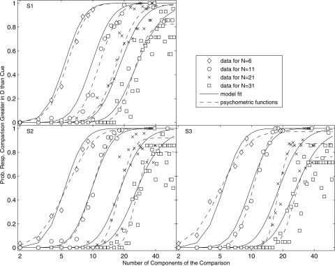
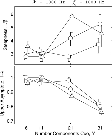
Figure 1 gives for each listener (panels) the individually fitted psychometric functions (dashed curves) and data (symbols) for the condition in which the number of tones in the cue N was varied holding the bandwidth and center frequency fixed (W = 1000 Hz and f_c = 1000 Hz). The continuous curves are fits of a model, which is discussed later. The functions are quite similar across listeners. For all listeners, the steepness of the functions increase with N, while the upper asymptote (1 − λ) decreases. The point where the functions give chance performance, $\stackrel{\wedge }{p}\left(N_c\right)=0.5$, also show a slight bias for all listeners (α < N), indicating a tendency to respond more often that the comparison was greater in density than the cue. The bias is unexplained; however, it did not affect the interpretation of the results and so is not considered further. The effect of N on the psychometric functions is evident in Fig. 2 where for each listener (different symbols) the steepness and upper asymptotes are plotted as a function of N. The figure reveals a transition region around N = 21 (corresponding to D = 0.021 Hz⁻¹) where the functions begin to change and where there is the greatest variability in the estimates of parameters across listeners.

Figure 1.

Shown for each listener (panels) are the psychometric functions relating the probability p of a “greater” response to the number of tones N + ΔN in the comparison for the condition in which the number of tones in the cue N was varied (different symbols). The bandwidth and center frequency for all N are fixed at respectively W = 1000 Hz and f_c = 1000 Hz. Dashed curves represent individual fits to the data for each condition and listener based on Eq. 4. Continuous curves give two-parameter fits to the data as a whole based on the frequency resolution model described in Sec. VII A.

Figure 2.

The steepnesses and upper asymptotes of the individually fitted psychometric functions in Fig. 1 are plotted as a function of the number of components N in the cue for each listener (S1 in squares, S2 in circles, and S3 in triangles). Confidence intervals for the fitted parameters shown were computed using the percentile bootstrap method based on 1999 simulations (Wichmann and Hill, 2001a,b). A slight horizontal offset has been added to the data for each listener to facilitate presentation.

These results differ from those of Neff and Green (1987) in that for the Weber fraction ΔN/N to be constant, the steepness of these functions must not change with N. However, as pointed out earlier, an important difference in procedure in that study is that the border frequencies were sampled at random along with the other frequencies. This means that, unlike the present study, the spectral density of the tone complexes varied from one presentation to the next in the Neff and Green study. To permit comparison to corresponding values of D in the present study, we can compute an expected value of D from the expected bandwidth of the tone complexes. For N frequencies sampled uniformly over the range R, the expected bandwidth is given by

$$E[W]=R\left(\frac{N-1}{N+1}\right).$$ (5)

In the Neff and Green study, the cue values of N ranged from 1 to 100, and the range over which frequencies were uniformly sampled was fixed at R = 5000 Hz. Hence, the expected spectral density,

$$E[D]=N/E[W],$$ (6)

in that study was never greater than 0.020 Hz⁻¹. Only these highest densities are close to the transition region around D = 0.021 Hz⁻¹ where the steepness of the functions begin to change. This could explain why Neff and Green observed a constant Weber fraction for the same values of N used in our study. Indeed, our functions for values of D < 0.02 Hz⁻¹ (for N = 6 and 11) yield a constant Weber fraction of ΔN/N ≈ 0.3, in rough agreement of the constant value of ΔN/N = 0.5 obtained by Neff and Green. If this explanation is correct, then allowing the border frequencies to vary in the present study, which results in a higher expected value of D, could possibly result in a decreased steepness of the psychometric function.

Effect of random border frequencies f_min and f_max

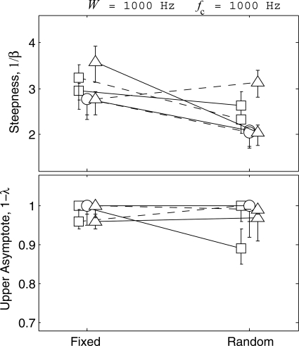
To evaluate the prediction in the preceding text, the same three listeners provided data for a second condition in which all N frequencies were uniformly sampled over the frequency range 500–1500 Hz. In all other respects, the conditions were identical to those for the case in which the border frequencies were fixed. The parameters of the psychometric functions for the three listeners for both fixed and random cases are shown in Fig. 3. Continuous and dashed lines give the data, respectively, for N = 6 and N = 11. With the exception of one listener in one condition (triangles, N = 11), allowing the border frequencies to vary has the expected effect of reducing the steepness of the psychometric functions. For the fixed condition, the steepness ranges from 2.7 to 3.8 across listeners and N; for the random condition the range is from 2.0 to 3.2. The later values yield a Weber fraction of ΔN/N ≈ 0.4, which is closer to the value of 0.5 obtained by Neff and Green (1987). The magnitude of the reduction in steepness, however, is not predicted from the change in the expected values of spectral density. From Eq. 7, we estimate E[D] in the random condition to be 0.008 Hz⁻¹ and 0.013 Hz⁻¹, respectively for N = 6 and 11. These values are only slightly greater than for the fixed case (0.006 and 0.011) and fall well below the transition region of D = 0.021 Hz⁻¹. Thus, based on the change in E[D] alone, no significant change in the steepness would be expected. It may be that E[D] is not the correct statistic for evaluating the central tendency of D in this case, or it may be that other factors, such as the added uncertainty associated with the random selection of border frequencies, is responsible for the difference in the steepness. Either way, the outcome does not change the conclusion that Neff and Green’s data were obtained for low values of D where one would expect from Fig. 2a constant Weber fraction for detecting changes in N.

Figure 3.

Same as Fig. 2 except the steepnesses and upper asymptotes of the psychometric functions are given for the conditions in which the border frequencies were fixed or were sampled at random with the other frequencies (f_c = 1000 Hz, W = 1000 Hz). Continuous and dashed lines represent, respectively, the conditions for which N = 6 and 11.

Effect of bandwidth and center frequency W and f_c

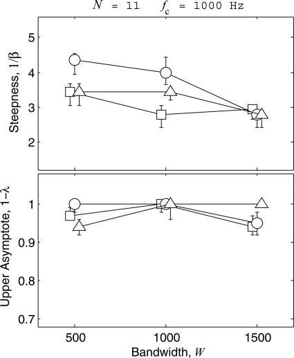
Figure 4 next shows the effect of bandwidth on the parameters of the psychometric functions. The number of tones in the cue was N = 11, and the center frequency of the bandwidth was f_c = 1000 Hz. The different symbols and curves represent the results from different listeners as before. The ordinate of each panel is scaled identically to that of Fig. 2 to permit comparison to the effect of N in Fig. 2. Over the range investigated, the effect of bandwidth on the psychometric functions appears much smaller than the effect of N. All three listeners show a reduction in the steepness of the functions from W = 500 to 1500 Hz. The reduction amounts to an average 0.8 unit change compared to a 1.5 unit change over the range of N in Fig. 2. There is also essentially no change in the upper asymptote, being close to 1.0 over the range for all listeners.

Figure 4.

Same as Fig. 2 except the steepnesses and upper asymptotes are for the condition in which the bandwidth W of the tone complexes was varied for a fixed center frequency f_c = 1000 and number of tones N = 11.

These results differ from those of Hartmann et al. (1986), who found performance to depend strongly on bandwidth. Although the bandwidths used in the Hartmann et al. study (50–800 Hz) differed from those of the present study; it seems unlikely that this alone could account for the discrepancy in results because the changes in performance observed by Hartmann et al. were significant even over the small range for which the bandwidths overlapped with the present study. A more likely explanation has to do, again, with the differences in D across the two studies. In the Hartmann et al. study, the number of tones in the cue was N = 60, yielding values of D = 0.075–1.2 Hz⁻¹. These values are well outside the transition region around D = 0.02, that is, the region where changes in D corresponding to changes in bandwidth would be expected to have an effect on the steepness of the psychometric functions. In the present study, by comparison, N = 11, yielding values of D = 0.007–0.022 Hz⁻¹—a range over which the steepness of the functions is expected to change. Hence the difference in results between the Hartmann et al. study and the present study might be understood in terms of the differences in D and its anticipated effect on the steepness of the psychometric functions within and outside of the transition region.

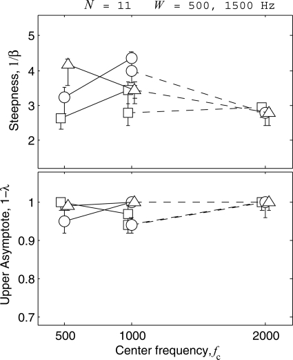
Finally, Fig. 5 shows the effect of center frequency on the psychometric functions. The number of tones in the cue was fixed at N = 11, the bandwidth was either 500 (continuous curve) or 1000 Hz (dashed curve). As for bandwidth, there appears to be little effect of center frequency on the psychometric functions. No consistent change in the steepness is seen across the three listeners, and the upper asymptote remains close to 1.0 for all listeners at all center frequencies.

Figure 5.

Same as Fig. 2 except the steepnesses and upper asymptotes are for the condition in which the center frequency f_c of the tone complexes was varied for a fixed bandwidth (W = 500 Hz, continuous lines; W = 1500 Hz, dashed lines) and number of tones N = 11.

These results agree with those of Hartmann et al., who also found little effect of center frequency on performance. The results are also in keeping with the hypothesis that D is the primary variable affecting performance inasmuch as D is constant for the two center frequencies for each bandwidth.

DISCUSSION

Our effort to this point has been devoted to documenting the effects of different factors (bandwidth, center frequency, and number of tones) on the ability of listeners to discriminate changes in the spectral density of multitone complexes. The data show discrimination performance to be determined primarily by the initial density D of the complex, all other variables affecting performance through their effects on D. The data also indicate a transition point, corresponding roughly to a value of D = 0.02 Hz⁻¹, beyond which the steepness of the psychometric functions relating performance to D increase and the upper asymptote decreases. The different behavior of the functions near and well above the transition point is consistent with the conclusions drawn regarding the effect of bandwidth and number tones, respectively, in the studies of Hartmann et al. (1986) and Neff and Green (1987). We next consider a model to account for these data.

Frequency resolution model

One factor that can be expected to influence a listener’s ability to discriminate changes in spectral density is their ability to resolve individual frequencies that make up the sound. At low levels of spectral density, where the frequencies of tones are widely spaced, a listener will be able to “hear out” the individual tones in the complex; this should aid in determining their number. As the level of spectral density increases, however, there must come a point where the individual tones are no longer separately resolved and the listener’s judgment regarding spectral density is affected. The simplest effect one could imagine is that two or more components, so closely spaced as to be unresolved, would be perceived as a single component, causing listeners to underestimate the true spectral density. This, in fact, is the basic premise of our model. Based on the data of Moore and Ohgushi (1993), we assume that at moderate sound levels the individual frequencies of the tone complex are resolved on an equivalent rectangular bandwidth (ERB) scale,

$$\mathit{ERB}(f)=108f+24.7.$$ (7)

where f is given in kilohertz (Moore and Glasberg, 1996). The first free parameter of the model, ω, is the smallest separation of components on this scale for which components are separately resolved (ω is expressed as a fraction of an ERB). Note here that the definition of “separately resolved” is principally the same as that of Moore and Ohgushi (1993) but differs operationally. Moore and Ohgushi determine ω to have a value of 0.75 in a task wherein listeners judged whether a pure tone was higher or lower in frequency than one of the tones in the complex. In the present application, ω determines the effective (i.e., perceived) density $\stackrel{\wedge }{D}$ on which listeners are presumed to base their judgments and so may take on a different value. The second free parameter is the steepness (1/σ) of a hypothetical psychometric function (cumulative normal) relating performance, or probability of a “greater” response, to changes in $\stackrel{\wedge }{D}$. The steepness is assumed to exhibit behavior consistent with Weber’s Law and so is constant for performance plotted against Δlog$\stackrel{\wedge }{D}$. The two free parameters ω and 1/σ interact to influence the shape of the empirical psychometric functions: For low values of D, where components are resolved, Δlog$\stackrel{\wedge }{D}$≈ ΔlogD, so the empirical functions follow the hypothetical functions; i.e., they have constant steepness and upper asymptote of 1.0. For high values of D, where components are unresolved, Δlog$\stackrel{\wedge }{D}$ approaches zero as D continues to increase; hence, the upper asymptote of the psychometric function is less than 1.0. The relation between D and $\stackrel{\wedge }{D}$ is further explained in the Appendix. This relatively simple model fits the data remarkably well as shown by the continuous curves in Fig. 1. For this result, single values of ω = 0.182 and 1/σ = 3.13 were used to fit the data of all listeners for all values of N. Although the model predicts changes in the steepness of the functions, the changes are small, hence the model predicts a roughly constant Weber fraction of 1/β = 0.32, which does a reasonable job in summarizing the data.

Application to the data of Hartmann et al. (1986)

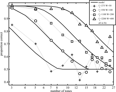
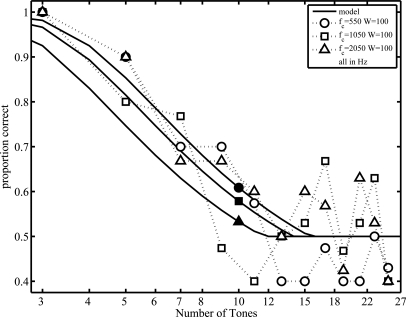
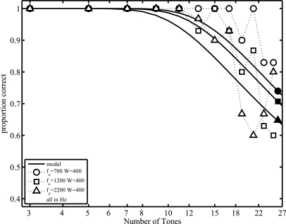
Hartmann et al. (1986) report in Fig. 1 of their paper complete psychometric functions for their listeners for N = 60 and different values of f_c and W. The average performance of these listeners is reproduced in Fig. 6. The values of f_c and W are, respectively, 300 and 50 Hz (pluses), 550 and 110 Hz (circles), 1200 and 200 Hz (squares), and 2400 and 400 Hz (triangles). Hartmann et al. also report for one listener (Figs. 23) psychometric functions for the condition in which f_c is varied for a fixed bandwidth. These data are reproduced in Fig. 7 where W = 100 Hz, f_c = 550 (circles), 1050 (squares), and 2050 Hz (triangles); and in Fig. 8 where W = 400 Hz, f_c = 700 (circles), 1200 (squares), and 2200 Hz (triangles). The data provide a strong test of the model as they include conditions for which spectral density is much higher than in the present study. Indeed, the strict application of the model, for which only ω and 1/σ was allowed to vary, produced quite poor fits to these data.

Figure 6.

Psychometric functions for spectral density discrimination representing the average of three listeners from Fig. 1 of Hartmann et al. (1986). The value of is N = 60, the values of f_c and W in different conditions are, respectively, 275 and 50 Hz (pluses), 550 and 100 Hz (circles), 1100 and 200 Hz (squares), and 2200 and 400 Hz (triangles). Continuous curves are fits to the data based on a model in which the cue for discrimination is assumed to be the rate of amplitude fluctuations of the time-envelope of signals (see Sec. VII B for details). Note that we use a logarithmic scale on the abscissa where Hartmann et al. used a linear scale (reproduced with permission).

Figure 7.

Psychometric functions for spectral density discrimination reproduced from Fig. 2 of Hartmann et al. (1986). The data are from a single listener. The continuous curves are 3-parameter fits of the temporal fluctuation model, same values of parameters as used for the fits in Fig. 6. (Reproduced with permission.)

Figure 8.

Psychometric functions for spectral density discrimination reproduced from Fig. 3 of Hartmann et al. (1986). Data are from the same listener as in Fig. 7. The continuous curves are fits of the temporal fluctuation model, same values of parameters as used for the fits in Fig. 6. (Reproduced with permission.)

The failure can be anticipated. As spectral density is increased, there must come a point at which decisions based on resolved components serve no advantage because none of the frequency components will be separately resolved. At this point, likely reached in the Hartmann et al. study, listeners must transition to a cue associated with the unresolved components if their performance is to be above chance. Hartmann et al. offer a model in which this cue is assumed to be the rate of fluctuations of the time envelope of unresolved components. The algorithm is explained in the appendix of their paper. Without doing the full calculation, we can see that this model differs in principle from the frequency resolution model in that it is frequency independent. The frequency independence is due to the fact that the rate of fluctuations depends only on the difference between frequencies not their absolute values. Therefore we might modify the frequency resolution model, effectively turning it into a generic rate of fluctuation model, by replacing the ERB function given by Eq. 7 with an alternative ERB function that is flat, i.e., is frequency independent. We refit the data of Hartmann et al. this time allowing the coefficient on frequency in Eq. 7 to vary as free parameters, b. The fits are given as the continuous lines in Figs. 67 ; the values of the fitted parameters are b = 6.25, ω = 0.23, and 1/σ = 0.50. These values are quite different from the previously obtained values, and this is to be expected because they are intended to reflect a different underlying detection cue. The fits are quite good. Moreover, as predicted, the value of b indicates near frequency independence, decreasing from an original value of 108 to an estimated value of 6.25. The failure to obtain complete frequency independence (b = 0) could reflect some residual influence of performance based on resolved components at the lower spectral densities in the Hartmann et al. study.

SUMMARY AND CONCLUSIONS

The present study investigated the effects of bandwidth, center frequency, and number of spectral components on the discrimination of changes in the spectral density ΔD of multitone complexes. The results indicate that these parameters affect the psychometric functions relating performance, or probability of a “greater” response, to ΔD through their influence on the initial value of D. For D < 0.02 Hz⁻¹, the steepness of the functions is constant, but at higher values, the steepness of the functions increases slightly and the upper asymptote converges to a value less than 1.0. These changes are predicted by a model where for low and moderate levels of D, performance is determined by resolved components on an ERB scale and a roughly constant Weber fraction of ΔD/D = 0.3. At much higher values of D, performance may be based on fluctuations in the time envelope of signals. The results should prove useful in evaluating the role of spectral density as a cue for determining the size and shapes of objects in studies of auditory sound source perception.

APPENDIX: THE DENSITY RESOLUTION MODEL

The density resolution model was used to describe our experiment’s data, as shown in Fig. 1, and those of Hartmann et al. (1986), as shown in Figs. 678. The main assumption of the model is that listeners cannot detect two tones separately if they are too close in frequency. We start by dividing the frequency spectrum into bands. The width of the bands was described in Sec. VII. The probability of at least one frequency component falling into each band was then calculated, and these probabilities then summed to find $\stackrel{\wedge }{D}$:

$$\stackrel{\wedge }{D}=\sum _i\min (1,E[\mathrm{components}\mathrm{in}\mathrm{band}i]).$$ (A1)

The probability that a component falls in a band depends on the way we generate the stimuli. For instance, for the stimuli used to generate Fig. 1, this would be

$$E[\mathrm{components}\mathrm{in}\mathrm{band}i]={\mathit{Dw}}_i,$$

except for the first and last band, which always have a component in them. The bandwidth of band number i is

$$w_i=f(i+1)-f(i),$$

where the boundary frequencies are calculated by using Eq. 7:

$$\begin{array}{c}\multicolumn{1}{c}{f(i+1)=f(i)+\omega \mathit{ERB}(f(i)),f(0)=f_{\min }.}\end{array}$$

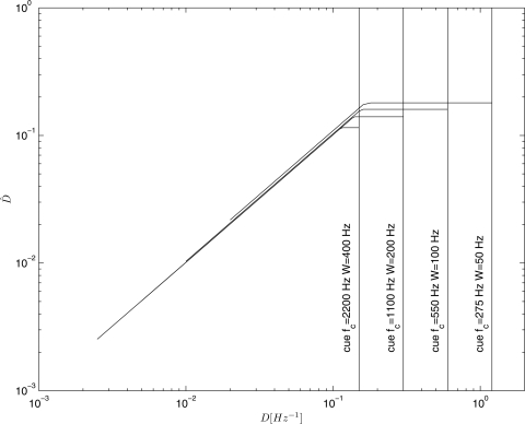
Because there could be more than one component in each band, $\stackrel{\wedge }{D}\le D$. When the density is low and the probability of two components falling in one band is low, $\stackrel{\wedge }{D}\approx D$; however, for some higher density, $\stackrel{\wedge }{D}$, will reach an upper limit, ${\stackrel{\wedge }{D}}_{\max }$ when at least one component falls in each band. The transition can either be gradual and abrupt, as we will see in Figs. 910.

Figure 9.

$\stackrel{\wedge }{D}$ as a function density (D), for the stimuli used to create Fig. 1.

Figure 10.

$\stackrel{\wedge }{D}$ as a function density (D), for the stimuli used by Hartmann et al. The four vertical lines represent the densities of the cue tones in various conditions. The cue tones are the endpoints of the four lines that represent the four functions that differ slightly in the varied conditions.

We calculated $\stackrel{\wedge }{D}$ numerically using the algorithm described in the preceding paragraph, for our data (Fig. 9), and for the data of Hartmann et al. (Fig. 10). Due to differences in experimental set up and the stimuli, the implementation of the model differed slightly for the two data sets. For the data used to create Fig. 1, the stimuli were the same for all the experiments, so there was only one function needed to calculate $\stackrel{\wedge }{D}$. The cue tone had 6, 11, 21, or 31 components per session, resulting in a different $\stackrel{\wedge }{D}$ for each session. These are shown in Fig. 9 as vertical lines.

Hartmann et al. used different center frequencies and bandwidths that resulted in slightly different functions for $\stackrel{\wedge }{D}$, (Fig. 10); However, differences in curves for the four conditions are minimal. The four conditions that were used to create Fig. 6 are shown in Fig 10.

Using Thurstone’s law of comparative judgments, we found the probability P_com>cue, indicating that the comparison is perceived greater than the cue. Because the psychometric functions were parallel on a log scale, shown in Fig. 1, we used $\overline{D}=\text{log}\left(\stackrel{\wedge }{D}\right)$:

$$P_{\mathit{com}>\mathit{cue}}=\Phi [{\overline{D}}_{\mathit{com}}-{\overline{D}}_{\mathit{cue}},\sigma ],$$ (A2)

where Φ[μ,σ] is the cumulative distribution function of a normal distribution with mean μ and standard deviation σ. The standard deviation was found by fitting the data as described in Sec. VII. In Fig. 1, P_com>cue is represented by a solid line. In the case of the data of Hartmann et al. (1986), the cue was always greater in density than the comparison, therefore 1 − P_com>cue is the proportion of correct answers, which is denoted by a solid line in Figs. 678. The region where ${\overline{D}}_{\mathit{com}}-{\overline{D}}_{\mathit{cue}}=0$ results in different offsets of the psychometric function for different conditions, as can be seen in Figs. 678.

References

- Bregman, A. S. (1990). Auditory Scene Analysis: The Perceptual Organization of Sound (MIT Press, Cambridge, MA: ). [Google Scholar]
- Hartmann, W., McAdams, S., Gerzso, A., and Boulez, P. (1986). “Discrimination of spectral density,” J. Acoust. Soc. Am. 79, 1915–1925. 10.1121/1.393198 [DOI] [PubMed] [Google Scholar]
- Kunkler-Peck, A. J., and Turvey, M. T. (2000). “Hearing shape,” J. Exp. Psychol. Hum. Percept. Perform. 26(1), 279–294. 10.1037/0096-1523.26.1.279 [DOI] [PubMed] [Google Scholar]
- Lutfi, R. A. (2001). “Auditory detection of hollowness,” J. Acoust. Soc. Am. 110(2), 1010–1019. 10.1121/1.1385903 [DOI] [PubMed] [Google Scholar]
- Lutfi, R. A. (2008). “Sound source identification,” in Springer Handbook of Auditory Research: Auditory Perception of Sound Sources, edited by Yost W. A. and Popper A. N. (Springer-Verlag, New York), pp. 13–42. [Google Scholar]
- Lutfi, R. A., and Oh, E. L. (1997). “Auditory discrimination of material changes in a struck-clamped bar,” J. Acoust. Soc. Am. 102(6), 3647–3656. 10.1121/1.420151 [DOI] [PubMed] [Google Scholar]
- Lutfi, R. A., and Stoelinga, C. N. J. (2009). “Sensory constraints on the identification of the geometric and material properties of struck bars,” J. Acoust. Soc. Am. 127(1), 350–360. 10.1121/1.3263606 [DOI] [PMC free article] [PubMed] [Google Scholar]
- McAdams, S. (1993) “Recognition of sound sources and events,” in Thinking in Sound: The Cognitive Psychology of Human Audition, edited by McAdams S. and Bigand E. (Clarendon, Oxford: ), pp. 146–195. [Google Scholar]
- McAdams, S., Chaigne, A., and Roussarie, V. (2004). “The psychomechanics of simulated sound sources: Material properties of impacted bars,” J. Acoust. Soc. Am. 115, 1306–1320. 10.1121/1.1645855 [DOI] [PubMed] [Google Scholar]
- Moore, B. C. J., and Glasberg, B. R. (1996).“A revision of Zwicker’s loudness model,” Acta Acust. 82, 335–345. [Google Scholar]
- Moore, B. C. J., and Ohgushi, K. (1993). “Audibility of partials in inharmonic complex tones,” J. Acoust. Soc. Am. 93, 452–461. 10.1121/1.405625 [DOI] [PubMed] [Google Scholar]
- Neff, D. L., and Green, D. M. (1987). “Masking produced by spectral uncertainty with multicomponent maskers,” Percept. Psychophys. 41, 409–415. 10.3758/BF03203033 [DOI] [PubMed] [Google Scholar]
- Rajalingham, C., Brat, R. B., and Xistris, G. D. (1995). “A note on elliptical plate vibration modes as a bifurcation from circular plate modes,” Int. J. Mech Sci. 37, 61–75. 10.1016/0020-7403(95)93053-9 [DOI] [Google Scholar]
- Rossing, T. D., and Fletcher, N. H. (1999). Principles of Vibration and Sound (Springer, New York), p. 75. [Google Scholar]
- Snijders, T. A. B., and Bosker, R. J. (1999). Multilevel Analysis: An Introduction to Basic and Advanced Multilevel Modeling (Sage, London: ), p. 49. [Google Scholar]
- Thurlow, W. R., and Rawlings, I. L. (1959). “Discrimination of number of simultaneously sounding tones,” J. Acoust. Soc. Am. 31, 1332–1336. 10.1121/1.1907630 [DOI] [Google Scholar]
- Wichmann, F. A., and Hill, N. J. (2001a). “The psychometric function. I. Fitting, sampling, and goodness of fit,” Percep. Psychophys. 64, 1293–1313. 10.3758/BF03194544 [DOI] [PubMed] [Google Scholar]
- Wichmann, F. A., and Hill, N. J. (2001b). “The psychometric function. II. Bootstrap-based confidence intervals and sampling,” Percept. Psychophys. 64, 1314–1329. 10.3758/BF03194545 [DOI] [PubMed] [Google Scholar]
- Wildes, R., and Richards, W. (1988). “Recovering material properties from sound,” in Natural Computation, edited by Richards W. (MIT Press, Cambridge, MA: ), pp. 356–363. [Google Scholar]