Hidden Markov Models for Zero-Inflated Poisson Counts with an Application to Substance Use

Abstract

Paradigms for substance abuse cue-reactivity research involve short term pharmacological or stressful stimulation designed to elicit stress and craving responses in cocaine-dependent subjects. It is unclear as to whether stress induced from participation in such studies increases drug-seeking behavior. We propose a 2-state Hidden Markov model to model the number of cocaine abuses per week before and after participation in a stress- and cue-reactivity study. The hypothesized latent state corresponds to ‘high’ or ‘low’ use. To account for a preponderance of zeros, we assume a zero-inflated Poisson model for the count data. Transition probabilities depend on the prior week’s state, fixed demographic variables, and time-varying covariates. We adopt a Bayesian approach to model fitting, and use the conditional predictive ordinate statistic to demonstrate that the zero-inflated Poisson hidden Markov model outperforms other models for longitudinal count data.

1. Introduction

Human laboratory paradigms for examining stress- or cue-reactivity in substance-dependent individuals often involve exposure to short-term pharmacological, social, or physical laboratory-based procedures or drug paraphernalia [1, 2, 4, 5, 6]. Although these studies are designed such that risks associated with participation are not outweighed by the importance of knowledge to be gained (e.g., improving treatment of future patients with drug dependence), stress contributes to drug-seeking behavior and increased risk of relapse [7, 8]. In particular, in an effort to determine underlying biological mechanisms of relapse among cocaine-dependent individuals, it has been shown that stress-related increases in cue-elicited craving result in a shorter time to drug relapse [9]. As minimizing risks to human subjects participating in clinical research is of paramount importance, we seek to determine whether participation in a clinical research study designed to induce stress and craving alters drug seeking behavior among cocaine-dependent individuals.

The DSM-IV symptoms[10] of substance dependence include the need for increasing amounts of the substance to maintain desired effects, withdrawal if drug-taking ceases, and a great deal of time spent in activities related to substance use [11]. Due to the detrimental impact of these behaviors, it is important to ensure that they do not increase after study participation as a result of study procedures. Consequently, ethical issues in substance abuse research have been widely studied, mainly with respect to coercion, ability to consent, and the influence ofmonetary reward on drug-seeking behavior [12, 13, 14, 15]. Using Time-Line Follow-Back (TLFB) data[14], compensating cocaine-dependent participants with cash did not result in increased rates of cocaine use during a one-month follow-up period. In fact, compensation has been shown to double the abstinence rate in smoking studies [16]. In an outpatient cocaine cue-reactivity study[17], 90% of patients had the same urine test results before and 3 days after cocaine cues, thus no detrimental effect was observed in patients immediately following testing. But to date, none of these studies have provided insight into longitudinal drug using behavior as a response to participation in non-treatment outpatient clinical research. As a result, it is still unclear whether participation in laboratory paradigms that invoke stress or craving could increase drug-seeking behavior or relapse among individuals with substance use disorders.

The motivating data for this paper come from an experiment performed on 45 cocaine-dependent participants that consist of daily diaries of cocaine use collected using the method of TLFB. In a study of alcohol abuse, [18] discuss why simple summary statistics are not adequate for modeling such self-reports of use over time. Such problems have also been discussed with respect to commonly used summary statistics in drug abuse [19]. For example, one commonly used summary variable, average dollar amount used per using day, does not differentiate from one person who uses moderately throughout the week and another who binges only on the weekend. The variable percent days used does not differentiate between light and heavy cocaine use. Another commonly used summary variable, time to relapse, is subject to censoring as a result of dropout and also requires a definition of relapse. Due to the loss of information in these summary measures or the introduction of censoring, which requires the use of survival analytic techniques, it is optimal to model the observed data at higher resolution, i.e., via daily or weekly observations, as opposed to one dimensional summary statistics. This will allow us to utilize the full data to model substance use longitudinally over many times points and will also enable us to make patient-specific predictions about drug abuse.

As drug-seeking behavior may be erratic due to various factors such as variable access to illegal drugs, social stigma, knowledge of impending drug testing and cost, it can be difficult to model serial drug use using standard longitudinal models for correlated data, such as linear mixed models. In particular, these high-dimensional serially correlated TLFB counts exhibit zero-inflation (ZI), are overdispersed, and dependent on possibly time varying covariates. The analytic challenges are summarized here:

1. At the top of Figure 1 is a chromatic plot of weekly drug use for the 45 cocaine-dependent patients enrolled in the above-mentioned study. The figure demonstrates a preponderance of zeros in that there are many days on which participants do not use cocaine. In addition, overdispersion is evident in these data in that the variance of the weekly counts increases faster than the mean count, violating the Poisson assumption.

2. We observed 16 weeks of serially correlated counts. Raw data auto- (and partial) correlations are shown in Figure 2 for 20 randomly chosen subjects. Autocorrelation is evident up to a potential time lag of 2 weeks for most of the subjects. Standard longitudinal methods such as generalized linear mixed models (GLMM) typically only handle a small number of time points because of the increase in the number of parameters required to explain the correlation structure. Typically in substance abuse studies, it is believed that the drug intake activity of a subject in a particular week might be highly dependent on the intake in the previous week (or weeks). This may not be readily handled using a random effects structure in the model or a multivariate structure for the response. Hence, there is a need to explore more sophisticated models assuming an alternative dependence structure.

3. Figure 1 (top) clearly demonstrates the sometimes erratic abuse patterns observed in cocaine-dependent populations. This may result in periods of consistent low level, or no use, punctuated by bursts of increased usage. Participants may use several times in one day or zero times in one week. This may result in several ‘outlying’ observations that we do not want to drive inference, however should be accounted for.

Figure 1.

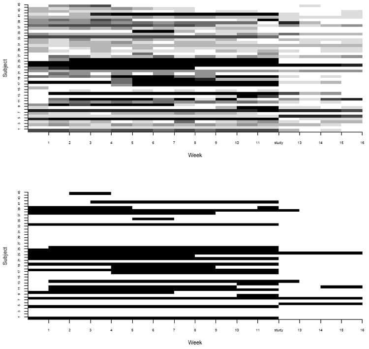
The top plot displays the matrix of weekly drug use counts for each participant in the study. White represents 0 days of use and shades of gray represent gradations in use. The bottom plot displays membership in the hidden state derived from posterior probabilities. White rectangles represent the low use state and black rectangles represent the high use state.

Figure 2.

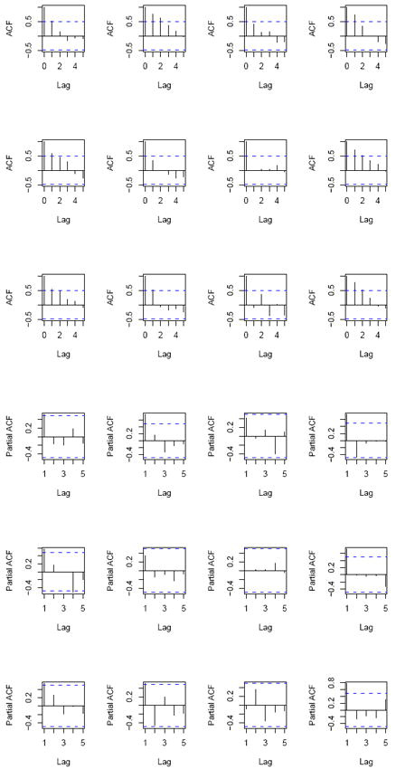
Raw data autocorrelation (ACF) and partial autocorrelation (PACF) plots for 12 randomly chosen subjects.

The preponderance of zeros problem in statistical modeling is well-recognized in the biomedical literature [20, 21, 22, 23, 24, 25] and in drug and alcohol consumption literature, in particular [26]. Here, commonly used Poisson regression models can underestimate the zero-count probability and hence make it difficult to identify significant covariate effects [27]. The zero-inflated Poisson (ZIP) regression model[28] is very useful for modeling those excess zeroes that cannot be explained by a Poisson distribution. Thus, we assume that weekly counts arise from a ZIP distribution [29].

To analyze the discrete time series at a high resolution, mitigate the effects of outliers, and account for measurement error inherent in self report, we propose a 2-state heterogeneous Hidden Markov Model (HMM) to reflect underlying, unmeasurable states of substance abuse. For each subject at each week, we hypothesize two underlying latent states corresponding to ‘high use’ and ‘low use’. These surrogate states have no predefined meaning or value, they are merely representations of frequency of use. Such latent constructs have been previously proposed to answer similar questions in the drug, alcohol, and psychiatry literature. For example, [30] analyzed binary longitudinal cocaine use outcomes using Markov transition models, [31] considered existence of an underlying healthy or unhealthy state based on the frequency of alcohol-related hospital visits, [18] hypothesized three underlying drinking states representing no drinking, light drinking, and heavy drinking based on daily usage data to analyze a longitudinal clinical trial of alcohol use disorders and [32] modeled underlying health states of schizophrenic patients in a longitudinal drug treatment study of just four time points. The common theme among all of these studies is the desire to model health status over time at an individual level. Similar approaches have also been proposed for the analysis of longitudinal count data in other biomedical applications, e.g., [33, 34].

In this paper, we adopt a Bayesian approach for the proposed HMM for ZIP counts because of its simplicity of exposition and ability to incorporate prior information in the presence of a large number of covariates that might potentially influence the ZI phenomenon. Although there is an artificial upper bound on the counts (due to data collection methods) for our motivating data, in general the number of uses in a week has no upper bound. In most substance use studies (in particular alcohol data), the fact that there is no upper bound underscores the need for accommodating zero inflated counts rather than zero inflated events/successes (e.g., through a zero inflated binomial, or ZI-BIN model). In the Discussion, we compare our fit to that obtained if the ZI-BIN were used and show that there is negligible difference in terms of prediction and mean squared error. Bayesian estimation relies on the MCMC[35] techniques for parameter estimation and is straightforward to implement in existing software, like WinBUGS. We assume that the probability of transitioning between states for a particular person in a given week depends on the prior week’s state, as well as fixed demographic variables and time-varying covariates, such as participation in the clinical study. The main research question is whether study participation alters drug seeking behavior. This question motivates the use of a change point model[36], as does the clear drop off in average weekly use at week 12 (study participation) shown in Figure 3. Further motivation for a change point will be discussed in Section 3.

Figure 3.

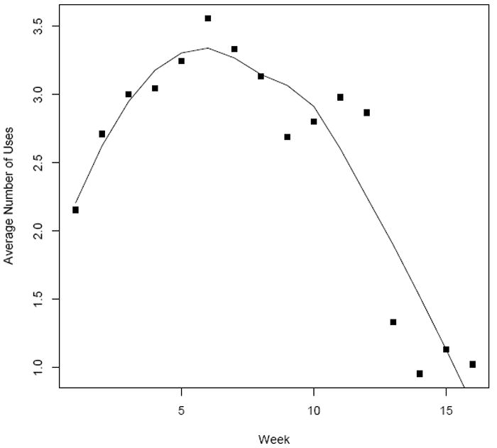
Averaged raw cocaine use data for the 16 weeks of the study. Curve represents the loess fit.

The remainder of the paper proceeds as follows. Section 2 provides a description of the motivating data. The HMM model for ZIP counts, along with competing models, is introduced in Section 3. Section 4 provides the estimation method using the Bayesian paradigm and issues related to prior specifications, model selection and goodness-of-fit. Section 5 presents results from model comparisons and summarizes the findings from data analysis. Discussions and future extensions are relegated to Section 6.

2. Cocaine Data

The 45 participants in this study were part of a larger, non-treatment study examining the relationship between stress reactivity, hypothalamic-pituitary axis functioning, and cocaine dependence. Participants were recruited in South Carolina via newspaper and other media advertisements. Following baseline assessment, participants underwent an overnight stay at the General Clinical Research Center (GCRC) at the Medical University of South Carolina where they were exposed to pharmacological and psychosocial laboratory stress tests. During the two-day hospital stay, three tasks were conducted: 1) the Trier Social Stress Task, 2) a pharmacological provocation (through administration of corticotrophin releasing hormone), and 3) a drug cue exposure paradigm (i.e., drug paraphernalia and a video depicting cocaine use). Before, during and after each stress task, neuroendocrine (e.g., cortisol) and physiologicalmeasures (e.g., heart rate) were obtained along with subjective reports of stress and craving. These data have been published in [38] who demonstrated the ability of these tests to elicit substantial subjective stress, craving, as well as physiological responses immediately after testing. Participants with elevated craving following testing procedures were required to stay in the hospital until craving subsided, and all participants were provided with resources for treatment programs in the community prior to discharge. Participants were discharged 2 hours following the last test and a follow-up visit was conducted 30 days after discharge during which participants were asked to provide detailed information about drug use since the testing. It was shown that in this cohort, increased stress reactivity was strongly associated with an increased risk of cocaine relapse [3]. The Structured Clinical Interview for DSM-IV was used to diagnose cocaine dependence [11] and the TLFB as described in Section 1 was used to assess the dollar value and frequency of cocaine use approximately three months before and one month after the study. This method has been show to provide accurate assessments of use in cocaine-dependent subjects [39]. Historical data were complete in all 45 subjects while follow-up data were missing on average, less than 10% of days. The mean [range] age in the study was 38 [20-53]. In addition, 44.4% were female, 46.7% were African American, 45.5% were employed, 54.5% attended some college, 80.0% were smokers, and 33.3% were married. Top panel of Figure 1 displays the TLFB daily usage for the 12 weeks prior to and 4 weeks after completion of the 2-day stress and cue-reactivity study.

3. Statistical Models

3.1. ZIP Hidden Markov Model for Poisson Counts

ZIP models are appropriate when the data exhibit overdispersion due to excess zeros as compared to a Poisson distribution. The total set of zeros in the data is a mix of ‘sampling zeros’ (those generated from the underlying Poisson process) and ‘structural zeros’ (the remaining zeros that are not originating from any process). This distinction relies on the result of a Bernoulli trial to dichotomize the study population into two sub-populations, viz. the low-risk group having the structural zeroes, and the high-risk (normal) group whose counts arise from a Poisson process [40]. This attractive feature naturally divides the total set of zero responses in the study population into the high and low risk subgroups. In the current study, such risks may depend on a variety of demographic variables.

We first present a heterogeneous zero-inflated Poisson HMM (ZIP-HMM) with subject-specific random effects that allows counts to move through the state-space according to covariate-specific transition probabilities, assuming a logit model for each row of the hidden state transition matrix. In the following, let Z_it represent the observed weekly drug use count and let the binary variable S_it denote the latent abuse state, which can take on two discrete values corresponding to high or low use, where i denotes patient and t denotes week; i = 1, …, N and t = 1, …, T. X_it and X_{T RTit} are the design matrices, representing fixed and possibly time-dependent covariates and treatments respectively. Note that there were no actual treatments administered in this particular study; the term ‘treatment’ simply refers to participation in the study, which is the main effect of interest in order to assess patient safety.

To develop the model, let S_it represent the ‘latent’ state of a two-state discrete time Markov chain where S_it = 1(0) denotes the high (low) use state. The ZIP-HMM model can be written as

$$\left(Z_{\mathit{it}}\mid S_{\mathit{it}}\right)=\{\begin{array}{ll}0& \mathrm{w}.\mathrm{p}.{\pi }_{\mathit{it}},\\ \mathrm{Poisson}\left({\theta }_{\mathit{it}}\right)& \mathrm{w}.\mathrm{p}.1-{\pi }_{\mathit{it}}\end{array}$$ (1)

with log(θ_it) = {λ_0i + λ_1iS_it−1}, where λ_0i and λ_1i are subject-specific random intercept and log ratio of the means in the high and low states for a given subject, respectively. For interpretation, exp(λ_0i) and exp(λ_0i + λ_1i) denote the mean number of days used per week in the low use group and high use groups respectively. Now, Z_it = 0 could represent either a structural zero (with probability π_it) or a sample zero (with probability 1 − π_it), where π_it is allowed to depend on covariates. The subscript i on the Poisson mean parameter allow for intra-subject heterogeneity[34]. We assume that given S_it = 1, the observed count Z_it follows a Poisson distribution with

$$f\left(Z_{\mathit{it}}\mid {\theta }_{\mathit{it}},S_{\mathit{it}}=1,X_{\mathit{it}},X_{T{\mathit{RT}}_{\mathit{it}}}\right)=\frac{1}{z_{\mathit{it}}!}{e}^{-{\theta }_{\mathit{it}}}{\theta }_{\mathit{it}}^{z_{\mathit{it}}}$$ (2)

where each unobserved binary T × 1 random vector (S₁, …, S_N) follows a 2-state discrete time hidden Markov chain with transition probabilities defined as

$$\begin{array}{lll}{p}_{\mathit{it}}^{00}& =& P(S_{\mathit{it}}=0\mid S_{i,t-1}=0,X_{\mathit{it}},X_{T{\mathit{RT}}_{\mathit{it}}})\\ p_{\mathit{it}}^{10}& =& P(S_{\mathit{it}}=1\mid S_{i,t-1}=0,X_{\mathit{it}},X_{T{\mathit{RT}}_{\mathit{it}}})\\ p_{\mathit{it}}^{01}& =& P(S_{\mathit{it}}=0\mid S_{i,t-1}=1,X_{\mathit{it}},X_{T{\mathit{RT}}_{\mathit{it}}})\\ p_{\mathit{it}}^{11}& =& P(S_{\mathit{it}}=1\mid S_{i,t-1}=1,X_{\mathit{it}},X_{T{\mathit{RT}}_{\mathit{it}}})\end{array}$$ (3)

for t = 2, …, T. Thus, the transition probability between two states at time t depends on the subject’s state at time t − 1, fixed and time varying covariates X_it, and time varying treatment X_{T RTit}. This dependence is clarified by writing the probability in terms of a logistic regression on the latent state,

$$p_{\mathit{it}}^{1S_{(i,t-1)}}={\mathrm{logit}}^{-1}({\beta }_0+{\beta }_1{S}_{i,t-1}+{\beta }_2{X}_{\mathit{it}}+{\beta }_3{X}_{T{\mathit{RT}}_{\mathit{it}}}).$$ (4)

For the current example, this probability represents the probability of transitioning to or remaining in the high use state given the covariates. The initial values, S_i1, for i = 1, …, N, are modeled as independent and identically distributed draws from a Bernoulli distribution with initial probability, p₀. We allow observed covariates (and possibly unobserved states, although not in this exposition) to predict the probabilities of the zero inflation phenomenon. This dependency is of interest as it allows us to identify low risk subgroups based on the covariates. Thus,

$$\mathrm{logit}({\pi }_{\mathit{it}}\mid Y_{\mathit{it}})={\alpha }_0+{\alpha }_1{Y}_{\mathit{it}1}+\cdots +{\alpha }_J{Y}_{\mathit{it\; J}}$$ (5)

where Y_it1, …, Y_{it J} are a set of J covariates that may or may not overlap with X_it in (2) and α₀ is an intercept. Rather than assuming all covariates are predictive of this process, we instead prefer to discriminate from a potentially large list of variables to avoid over-parameterization. To identify a subset of the J covariates that are useful in predicting the zero inflation process, we consider an informative double exponential (DE) prior (also called a Laplace prior) on the coefficients in Equation 5. Such priors are frequently used for variable selection in regression to give the Bayesian estimates of the lasso [41]. How well the parameter is differentiated from zero will determine how well that variable is predictive of the zero state. Prior selection will be discussed further in Section 4.1.

3.2. Other Hidden Markov Models

Addition of subject-level random-effects in a HMM framework is a natural extension[34] that accounts for other intra-subject heterogeneity. The random effects that we specify accommodate the individualized nature of the diagnosis of cocaine dependence by giving the underlying latent variable a subject-specific definition. We compare our ZIP-HMM to a model without zero inflation [31] and with and without random effects. The ‘Wall and Li’ model[31] assumed that Z_it∣θ_it, S_it, X_it, X_{T RTit} is Poisson distributed, i.e.

$$P\left(Z_{\mathit{it}}\mid {\theta }_{\mathit{it}},S_{\mathit{it}},X_{\mathit{it}},X_{T{\mathit{RT}}_{\mathit{it}}}\right)=\frac{1}{z_{\mathit{it}}!}{e}^{-{\theta }_{\mathit{it}}}{\theta }_{\mathit{it}}^{z_{\mathit{it}}}$$ (6)

where θ_it = log(λ₀ + λ₁S_i,t−1) where transition probabilities between hidden states are defined as in Equation 3. This model[31], originally conceived to assess outpatient alcohol-related hospital visits, is not directly applicable to modeling illicit drug use due to the erratic nature of cocaine use in our study. In addition, the diagnostic criteria for drug dependence depend on individual behaviors and not necessarily on amount or frequency of use. For example, although two people exhibit the same use pattern, only one person may be deemed by DSM-IV criteria to be drug-dependent. From hereon in, we will call the ‘Wall and Li’ model with (without) random effects as ‘Wall (RE)/(no RE)’ model. Similarly, we will use the terminology ZIP-HMM (RE) and ZIP-HMM (no RE) to distinguish the ZIP-HMM with and without random effects.

3.3. Modeling the Time Trend After the Study

Figure 3 plots the average number of cocaine uses versus week with the overlayed LOWESS curve for the 16 weeks of study. Study participation occurred at time, t_s = 12 after which there appears to be an immediate drop off in use. Further, fitting a simple lagged Poisson regression with a time dependent study effect to these data resulted in a highly significant study effect on use behavior. This motivates consideration of a semi-continuous ‘change-point’ model[36] to model the time-dependent effect of participation on the transition activities. A priori, we expect the effect of time on transition activity to be altered by participation in the study and potentially allow for this trend to change as participants become further removed from the day of participation. To provide more flexibility in studying the nature of effects generated by the change-point, we expand on the treatment covariate effect in Equation 4 by including not only the binary indicator of change-point but also associated linear and quadratic terms as,

$${\beta }_3{X}_{T{\mathit{RT}}_{\mathit{it}}}={\beta }_{O}I(t\ge t_s)+{\beta }_L(t-\overline{t})I(t\ge t_s)+{\beta }_Q{(t-\overline{t})}^{2}I(t\ge t_s),$$

Introduction of the parameters β_O, β_L and β_Q allow us to characterize the effect of study participation and to determine whether or not it provides a lasting preventative or detrimental impact. The change-point term I(t ≥ t_s) accommodates a sudden change in the response profile at time t_s, while the associated linear and quadratic terms determine the trend (nature and extent) of the change and whether it dies off or not.

3.4. Nested Models

To both compare and further motivate the need for multi-state latent variables for analyzing the data, we considered nested, or ‘1 state’ models. We fit four nested lagged models including first and second order autoregressive (AR) and autoregressive error models[37], all of which included the aforementioned fixed and time dependent covariates. Based on the lag, these can be denoted AR(1), AR(2), AR(1) error, and AR(2) error models ([37, 42]. The simple AR(1) and AR(2) include a covariate term for the count at the previous one or two time points, e.g., Z_it∣θ_it ~ Poisson(θ_it) where log(θ_it) = γ₀ + ρ₁Z_i,t−1 + γ₁X_it + γ₂X_{T RTit} + u_it, where the errors u_it are exchangeable white noise ~ N(0,σ²), and Cov(u_is, u_it) = 0. The AR(1) error model takes the form Z_it∣θ_it ~ Poisson(θ_it) where log(θ_it) = γ₀ + γ₁ X_it + γ₂X_{T RTit} + ∈_it. Here, we let ∈_it = ρ₁ ∈_it−1 + U_t for i = 1, …N and t = 2, …, T, and let ${\mathit{\in }}_{i1}=\frac{U_1}{1-{\rho }^2}$ as in [42]. In this formulation, U_t for t = 2, …, T, is assumed to be normally distributed with mean 0 and variance ϕ², for which a hyperprior is specified for Bayesian inference. Consecutive error terms are assumed correlated for the nonzero portion of the ZIP model, where the strength of the correlation parameter ρ₁ lends insight into the autoregressive nature of the error terms. Given the potential autocorrelation of the raw data up to time lag of week 2 as shown by the autocorrelation plots in Figure 2, we similarly fit a second order autoregressive AR(2) error model with an additional parameter ρ₂ of the form ∈_it = ρ₁ ∈_it−1 + ρ₂ ∈_it−2 + U_t for t = 3, …, T. We note that for a AR(p) (p^th order autoregressive) process to be stationary, the constraint |ρ₁ + ρ₂ + … + ρ_p| < 1 must be applied.

4. Bayesian Inference

We adopt a Bayesian approach to model fitting, which requires the specification of prior distributions for all unknown parameters. This has several advantages over a likelihood-based frequentist approach. An Expectation-Maximization (EM) algorithm using forward backward recursion is a viable alternative for HMM parameter estimation but is slow to converge and requires multiple runs from several initial points in the parameter space. Besides the ability to incorporate prior information, the Bayesian paradigm uses the Gibbs sampler and MCMC algorithms to determine estimates of an exact posterior distribution. In our case although the posterior distribution of the model parameters cannot be computed analytically, this can be easily automated within WinBUGS Version 1.4.3 [43]. The code is available upon request from the first author. We ran 2 chains with widely dispersed starting values to assess convergence. Due to the complexity of the ZIP-HMM model which consists of nested mixtures, parameter convergence was achieved at a relatively high burn-in size of 40,000 iterations. Discarding these burn-in samples, we monitored the posterior distribution of model parameters over 40,000 further iterations, saving every second sample in the chain to reduce autocorrelation in the MCMC simulation. The length of burn-in and monitoring was determined by assessing trace and autocorrelation plots and the Gelman-Rubin potential scale-reduction factor, R̂ [44]. With these specifications, the chains took approximately 20 minutes to converge using a Windows XP, 32-bit, Dell workstation with Pentium 4, 2.40 GHz dual processors and 2G of RAM.

4.1. Prior Specification

Where variable selection was not of interest, we specified noninformative prior distributions for the model parameters. For the HMM’s presented in Section 3, we specified the following non-informative priors: β₀, β₁, β₂, β_O, β_L, β_Q ~ N(0,σ²=100). The parameters λ_0i ~ Gamma(0.01,0.01) and λ_1i ~ Gamma(0.01,0.01), where Gamma(a, b) is the density of a Gamma distribution given by $f_{a,b}(x)=\frac{b^a}{\mathrm{\Gamma }(a)}\exp (-\mathit{bx})x^{a-1}$. Where random effects weren’t included, we specified λ₀, λ₁ ~ Gamma(0.01,0.01). For the ZI model, we specified f₀ ~ Bernoulli(π_it), where π_it is as in Equation 5. In all models, the prior for the initial transition probability was, p₀ ~ Beta(1,1). For the AR models, we specified γ₀, γ₁, γ₂, γ_O, γ_L, γ_Q ~ N(0,σ²=100), ϕ ~ N(0,σ²=100). To select a subset of covariates predictive of the ZI process, we used an informative double exponential (DE) prior, such that if β ~ DE(0, τ), then the p.d.f of β is $\frac{\tau }{2}\exp (-\tau \left|\beta \right|)$ for −∞ < β < ∞, and variance 2/τ². The DE prior was centered at 0 to reflect a skeptical view about parameter effects and requiring strong evidence from data a posteriori to suggest otherwise. Thus for the parameters determining the zero inflation probability, we specified α₀ ~ N(0,σ²=100) and the vector of parameters, α₁ ~ DE(0,1).

Another approach to identify a subset of the J covariates that are useful in predicting the zero inflation process is to embed a ‘spike and slab’ mixture prior [45] to study the effect of the covariates on the logit probabilities in Equation 5. Such priors are frequently used for variable selection in linear and logistic regression [46]. As we already specified a ZI mixture at the level of modeling the time series as well as a binary latent variable reflecting hidden state, introducing another mixture might run the risk of model over-parameterization. Thus in the interest of parsimony, we imposed an informative DE prior to achieve variable selection.

4.2. Selecting the Order of the HMM

To determine the appropriateness of a p^th order Markovian structure for our HMM, we first examine the raw autocorrelation function (ACF) and partial correlation function (PACF) for each individual in the sample to visually assess the correlation at various time lags, up to a lag of 5 (Figure 2). The plots reveal presence of a strong first order and a possible second order dependence, however, both the correlation and partial correlation decrease rapidly with increasing time lag of p ≥ 3. Next, we explore several nested (i.e., ‘1- state’) models in order to further discern the autoregressive nature of the data, as well as to motivate the need for the assumption of a p^th order Markovian structure. The simplest model that we considered was a lagged Poisson regression as described in Section 3.4 where we tested several time lags. Results from this models based on posterior mean and associated 95% credible intervals (C.I.) were consistent with the raw ACF and PACF plots, as they indicated the need for a first and second, but not third order dependency. Finally, we fit AR(1) and AR(2) error models to the data as described in Section 3.4 assuming a ZIP structure to accommodate over-dispersion.

4.3. Model Selection and Assessment

We compared the four competing models discussed in Section 3, i.e., (a) theWall model, (b) the Wall model with random effects (RE), (c) the ZIP-HMM and (d) the ZIP-HMM with RE. We also compared these HMMs with the nested models. Although a variety of model selection procedures exist in the Bayesian toolbox, there is dearth of any unanimous ‘correct’ approach for model selection [44]. Thus our model comparisons are based solely on predictive performances of competing models. If Θ denotes the entire parameter space of our model and Z_pr denotes the predictive data vector, then the posterior predictive distribution (p.p.d) is given by:

$$p(z_{\mathit{pr}}\mid z)=\mathit{\int }p(z_{\mathit{pr}}\mid \mathrm{\Theta })p(\mathrm{\Theta }\mid z)d\mathrm{\Theta }$$ (7)

where predictive data are easily obtained from converged posterior samples. The basis for our model selection is the conditional predictive ordinate (CPO) statistics, a widely used tool for Bayesian model diagnostic and assessment [47, 48, 49]. Importantly, it is useful in evaluating model fit when the Bayesian deviance information criteria (DIC)[59] is difficult to calculate. The CPO is calculated as a ‘leave-one-out’ cross validation predictive density. As it provides a quantitative measure for the effect of observation i on the overall prior predictive density, small CPO values indicate observations that are not expected under the cross-validation predictive distribution of the current model; larger values implies that the data point is consistent with the current model. Defining D⁽ⁱ⁾ to be the covariate data for the ith subject, letting D⁽⁻ⁱ⁾ be the covariate data for all subjects except the i^th subject, and letting Θ represent the parameter space, it follows that the CPO statistic for the i^th subject is

$$\begin{array}{lll}{\mathrm{CPO}}_i& =& p(z_i\mid D^{(-i)})\\ & =& \mathit{\int }p(z_i\mid \mathrm{\Theta },D^{(i)})\pi (\mathrm{\Theta }\mid D^{(-i)})d\mathrm{\Theta }\end{array}$$ (8)

where π(Θ∣D⁽⁻ⁱ⁾) is the posterior distribution of Θ under the prior, π(Θ). Due to the lack of a closed form solution to (8), a Monte Carlo approximation[48] for observation i can be obtained from G iterations of the Gibbs sampler as,

$$\widehat{{\mathit{CPO}}_i}={\left(\frac{1}{G}\sum _{g=1}^G\frac{1}{p\left(z_i\mid {\mathrm{\Theta }}^{(g)}\right)}\right)}^{-1},$$ (9)

where Θ^(g) denote the parameter samples at the g^th, g = 1, …, G iteration of the Gibbs sampler. Plots of -log(CPO_i) values for i = 1, …, N provide evidence of the predictive performance of the competing models. Smaller values of -log(CPO_i) indicate better support for the model from observation i. To compute an overall summary measure of model fit, the log pseudo-marginal likelihood (LPML) statistic is obtained by evaluating ${\sum }_{i=1}^N\log (\widehat{{\mathit{CPO}}_i})$. Thus, a larger LPML value indicates a better support of the model from the aggregated observed data.

4.4. Goodness-of-Fit

The goodness-of-fit of the selected model was assessed by calculating the posterior predictive p-values [44], which measures the discrepancy between the data and the model by comparing a summary statistic of the p.p.d to the true distribution of the data. To accomplish this, we calculated χ²(z, θ^g) and χ²(z^rep,(g), θ^g), where z^rep denote the replicated value of z from the p.p.d at the g^th iteration of the Gibbs sampler. The posterior predictive p-value is then calculated as P(χ²(z^rep,(g), θ^g) > χ²(z, θ^g)), i.e. the proportion of times χ²(z^rep,(g), θ^g) exceeds χ²(z, θ^g)) out of g = 1, …,G simulated draws from the p.p.d. This Bayesian p-value, as determined by the tail-area probability, measures the lack of fit of the data with respect to the p.p.d, and is a good indication of whether the variation in the data is consistent with the variation predicted by the model[51]. This measure can be computed within WinBUGS using posterior simulations of the data and model parameters. A Bayesian p-value in the range 0.05-0.95 indicates a reasonable fit, while a very large (>0.95) or a very small (<0.05) p-value signals model misspecification, i.e., the observed pattern would be unlikely to be seen in replications of the data under the true model [44].

5. Results

Figure 4 is a plot of ordered -log(CPO_i) statistics for three of the nested 1-state models, i.e. the AR(1), the AR(1) error, and AR(2) error models. The AR(2) error model resulted in the best performance of nested models. This model demonstrates consistently smaller -log(CPO)_i values and a larger LPML (-1053.5) as compared to the AR(1) (LPML= -1166.4). Further, the CIs of both autocorrelation parameters excluded the null value.

Figure 4.

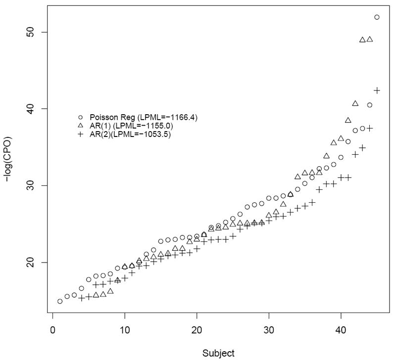
Relative model fits of nested models based on -log(CPO_i). The value in parenthesis is the LPML (larger is better).

Next, we fit four second order HMM’s, i.e. (a) the Wall model, (b) the Wall model with RE, (c) the ZIP-HMM, and (d) the ZIP-HMM with RE to the longitudinal cocaine use data. Figure 5 is a plot of ordered -log(CPO_i) statistics for each subject for each model; LPML is also reported. While there is some overlap of -log(CPO_i) values across the two ZI models, the LPML is the largest for the ZIP-HMM with RE (LPML = -1013.3), implying that this model provides the best predictive fit. In fact, according to the LPML and even individual CPO’s, there is a clear progression of model performances, with the most basic model from [31] without RE exhibiting the worst and stepwise improvement when incorporating RE and a model for ZI. We surmise that as one incorporates RE and ZI, individual observations become more consistent with the model. The residual ACF and PACF from the 2-state, second order ZIP-HMM behaved like white noise with zero mean and constant variance, revealing that the model fit is adequate and optimal. Compared to all HMM’s, the worst LPML calculated was for the lagged Poisson model. This may be a result of the fact that the HMM tempers the highly positive estimation of the time lag effect through the introduction of a latent variable that better handles measurement error inherent in self report, and better accommodates the natural variation in the weekly counts. Notably, for the lagged Poisson model, the effect of the prior count on the current count resulted in a significant posterior mean [95% Credible Interval], exp(γ₁) = 1.28 [1.25, 1.30]. This tight interval characterizes the strong week to week dependency in drug using behavior. As discussed in [31], due to the strong estimated lagged effect in the Poisson regression model, if there are a high number of uses in a particular week, the nested model will predict a similar high number of uses in the next week, which has a tendency to overestimate the number of uses when specific high values do not persist. Henceforth, we present results from the ZIP-HMM with RE fitted to our data.

Figure 5.

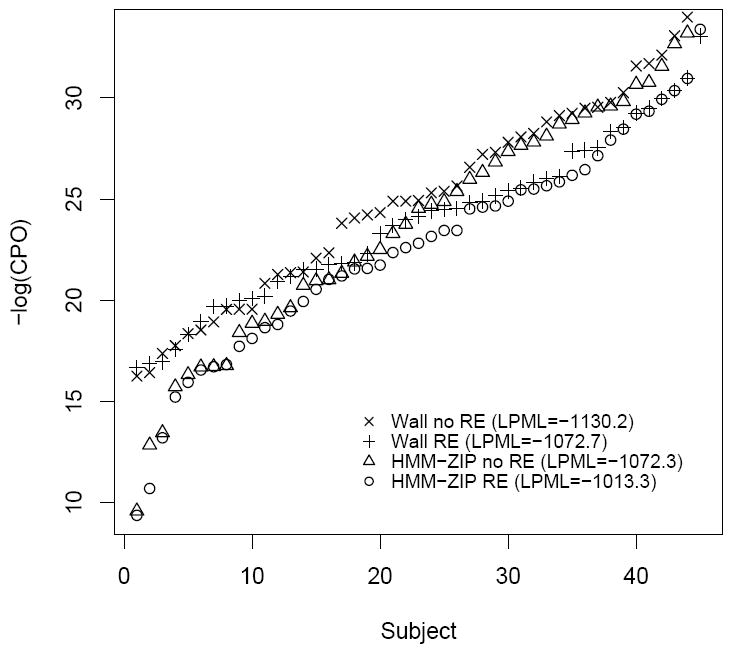
Relative model fits of the 2-state hidden Markov models based on -log(CPO_i). The value in parenthesis is the LPML (larger is better).

The posterior predictive p-value for the ZIP-HMM model with RE was 0.36, implying that the model is consistent with the observed data. Visual inspection of trace plots for importantmodel parameters demonstrated a sufficient burn-in period (Figure 6). Autocorrelation plots of important model parameters (Figure 7) up to a time lag of 20 iterations indicated that the thinning of the chains employed was sufficient. Unless otherwise noted, results are presented as posterior mean odds ratio (OR) [95% C.I.].

Figure 6.

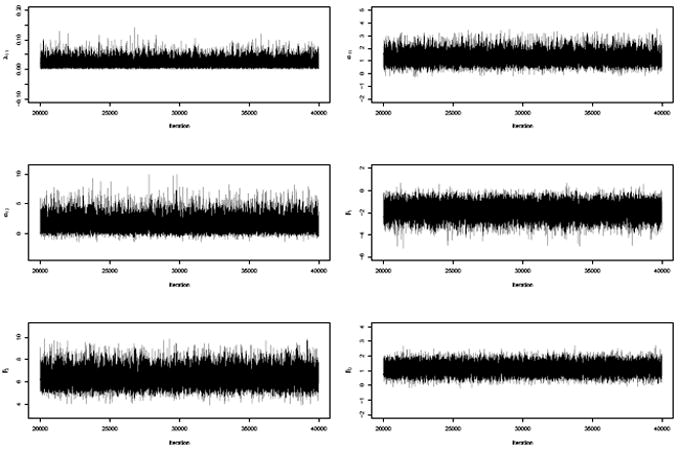
Traceplots of some important parameters from the 2-state ZIP-HMM model showing adequate mixing of the MCMC chain.

Figure 7.

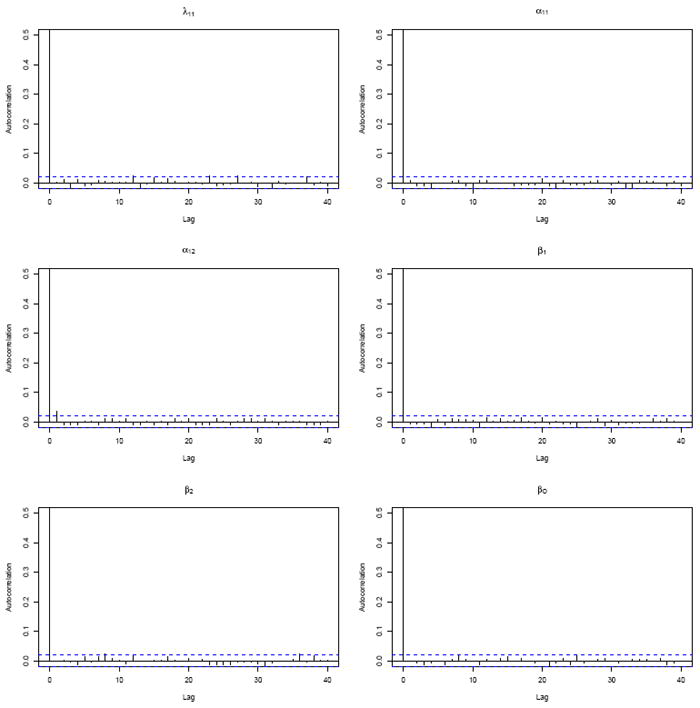
Autocorrelation plots from the 2-state ZIP-HMM model for various time lags showing adequate thinning of the MCMC chain occurs with every 2 draws.

As expected, due to serial autocorrelation, an individual’s prior state is significantly predictive of their current state, thus the odds of transitioning between high and low use states in general are low in this population. The log OR of remaining in the high use state at time t given that the subject is in the high use state at time t − 1 is 6.46 [5.02, 8.29]. This provides justification for considering a HMM to derive latent constructs for serially correlated counts of cocaine use. The population ‘mean number of days use per week’ for participants in the high use state is 3.4 versus 1.0 days in the low use state. Table 1 displays the OR’s and 95% C.I. for covariates used in modeling the ZI and transition probabilities, respectively. The odds of transitioning to or remaining in the high use state in any given month after participation in the study was OR_{T RTO} = 0.06 [0.01, 0.19] of what it was in the 12 weeks prior to the study. As this 95% CI excludes 1, it provides evidence of a substantially protective effect of study participation on subsequent drug use. Inversely stated, the odds of remaining in or transitioning to the low use state after versus before the study is 1/.06 = 16.7. This highly preventative effect of study participation on use behavior is illustrated in the bottom of Figure 1. To construct this figure, participants were assigned to the hidden state for which they had the highest posterior probability of membership at each time point. The figure displays the hidden state at each time point for each participant in the study, where black rectangles represent the high use state and white rectangles represent the low use state. Accounting for covariate effects, the study-specific benefit (seen after week 12) in reducing drug-seeking behavior is evident by the preponderance of white rectangles in the figure.

Table 1.

Odds ratios and 95% credible intervals illustrating the odds of zero inflation, and the odds of remaining in or transitioning to the high use state obtained from fitting the ZIP-HMM.

Variable (Zero Process)	Posterior Mean Odds Ratio	95% Credible Interval
Gender(M:F)	20.0	2.88, 90.00
Age†	0.29	0.10, 0.69
Race (AA:White)	4.41	0.81, 80.16
Smoker (Y:N)	12.51	2.13, 100.03
Variable (Transition Probabilities)
TRTO	0.06	0.01, 0.19
TRTL	1.91	1.30, 2.87
Gender(M:F)	0.76	0.25, 2.44
Age†	1.67	0.91, 3.15
Race (AA:White)	1.43	0.47, 4.66
Smoker (Y:N)	0.51	0.17, 1.52

^*95% Credible Interval excludes 1

^†Odds ratio for a 1 standard deviation increase

AA = African American race

As there were too few weeks after the study to capture a quadratic time trend and the 95% C.I. did not exclude 1, the quadratic term was dropped from all models so as not to obfuscate the effect of other treatment covariates, TRT_O and TRT_L. Estimates for linear trend implies a linear increase in the odds of remaining in or transitioning to the high use state after participation in the study (OR_{T RTL} = 1.94 [1.28, 2.92]). We do note however that the posterior mean treatment effect is so strong that even by the fourth week after the study ended, participants do not rise up to their pre-study odds of transitioning. Another way to quantify the effect of participation on transition behavior is to observe the posterior distribution of relevant transition probabilities, p₁₁ and p₁₀. These distributions illustrate the probabilities of remaining in the high use state, and transitioning to the high use state, respectively. In Figure 8, the distributions are plotted for 3 representative subjects in the dataset, before (solid) and after (dashed) participation in the study. It is clear from both sets of transition distributions p₁₁ and p₁₀ that the probability of remaining in or transitioning to the high use state decreases markedly after participation in the cue reactivity study. Of greatest note is that participants are much less likely to remain in the high use state after study participation than they were prior to study participation, thereby illustrating the strong effects of study participation on use behavior. The remainder of the subjects demonstrated very similar profiles.

Figure 8.

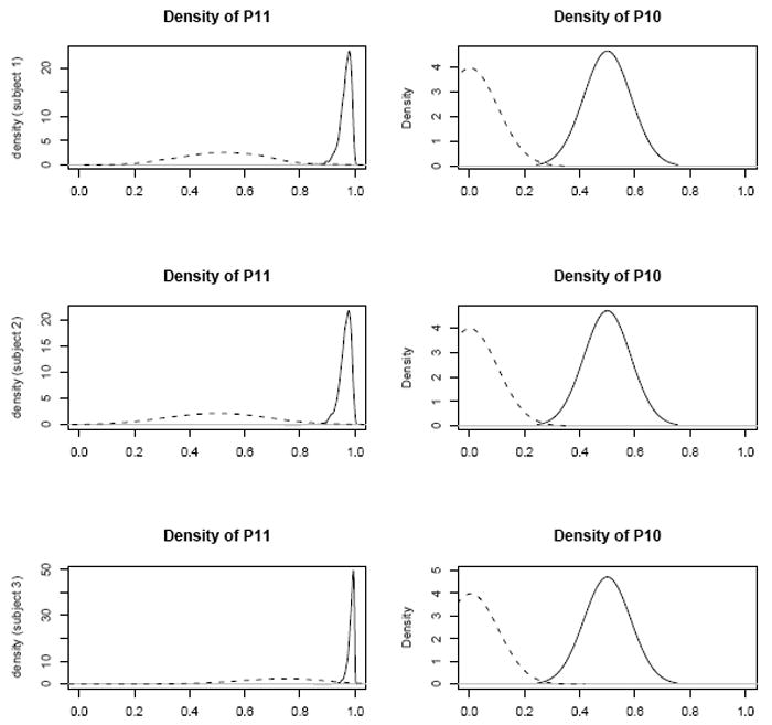
Posterior density of probability of remaining in the high use state (p¹¹) and probability of transitioning into the high use state (p¹⁰) before (solid) and after participation in the study (dashed)

As the 95% CI for gender, age and smoking status excluded the null value of 1, these covariates are predictive of whether observations arise from the zero process. Gender (OR = 20.00 [2.88, 90.00]), smoking (OR = 12.51 [2.13, 100.03]) and age (OR=0.29 [0.10, 0.69]) are all predictive of structural zeros and hence males, smokers, and younger participants are among the low risk subgroup. Although from a substantive point of view, it might seem nonintuitive that males and smokers are less likely to abuse cocaine, this finding is consistent with empirical observations of these data. For example, men used cocaine an average of only 37 days while women used an average of 44 days during the 112 day study. Similarly, smokers used cocaine an average of only 38 days while nonsmokers used an average of 47 days. When reporting covariate effects, it is important to note that this was an observational study with a limited sample size that resulted in some imbalance in covariates/risk factors in the sample. For example, 80% of participants were smokers (as is common in studies of substance abuse), which unfortunately limits inference for this covariate.

We note that while these covariates were predictive of structural zeros, no covariates meaningfully influenced the odds of transitioning between states, as all 95% CI included 1. This was not the case for the Wall model, i.e., when ZI was not explicitly modeled. Results from fitting the Wall model (with or without RE) indicated that both age and smoking had an effect on the odds of transitioning, but the ZIP-HMM model demonstrated that these covariates are actually more predictive of the zero process, i.e., they identify low-risk subgroups. This comparison underscores the fact that ignoring ZI can underestimate the zero-count probability and hence make it difficult to identify important covariate effects.

For the purpose of describing the effect of the non-treatment study on cocaine abuse, we a priori defined a ‘full study effect’ as being assigned to the high use state for all four weeks immediately before the study, but for zero weeks after the study. According to the model, 19 (42%) participants actually exhibited a full study effect. Moreover, the bottom of Figure 1 demonstrates that most participants evidenced a beneficial effect of participation in the study, while only a few had no obvious change in pre-study behaviors.

Finally, a sensitivity analysis to prior variance specification was performed. Results were not sensitive to more noninformative (larger than 100) choices of the variance of the normal priors, as measured by posterior state memberships for each individual at each time point as well as posterior mean parameter estimates for fixed effects. Results were also not sensitive to the order of the HMM. To justify the need for a set of subject-specific random effects (as suggested by a reviewer), we plotted the marginal posterior distribution of the random parameter λ_1i, for 16 random subjects in Figure 9. The posteriors vary considerably across subjects and hence conditioning on this parameter is essential to accurately characterize average using behavior.

Figure 9.

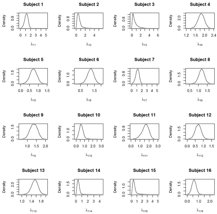
Posterior distributions of random parameters λ_1i

6. Discussion

The goal of this study was to determine whether participation in a non-treatment outpatient clinical study is protective or detrimental in terms of frequency of follow-up drug use among cocaine-dependent participants and to determine relevant demographic predictors of use parameters. This question is of ethical importance to researchers enrolling drug-dependent individuals into studies where they will be exposed to pharmacological and social stressors. It is also of interest from a treatment standpoint in that increased awareness resulting from participation alone may affect substance using behavior.

The top panel of Figure 1 demonstrates that there are clear subpopulations of cocaine users, including those who consistently abuse cocaine less frequently throughout the study, yet who stillmeet the criteria for cocaine-dependence. This preponderance of structural zeros, as well the lack of fit of the HMM with the standard Poisson structure for the discrete time series, is the motivation for the current paper. The HMM presented here is a natural way to derive an underlying use state. It accounts for ZI in the number of cocaine uses per week, allows for measurement error between the self reported events and underlying latent states, and mediates the effect of outlying observations. This novel formulation extends previously proposed HMM for alcohol abuse introduced in [18, 31] by considering a random effects HMM for ZIP counts of weekly drug use, with skeptical prior assumptions on the zero-generating process. This approach improves substantially upon commonly used nested 1-state models, which are much less sensitive in detecting weekly variations when high or low values do not persist in the data. In addition, we presented a basis for model comparison motivated by Bayesian arguments via CPO’s. Results of fitting the ZIP-HMM showed that participation in the study was highly protective against transitioning to the high use state. In fact, if our hypothesized latent variable is to be believed, then our observed post-study ‘response rate’ of 42% mirrors abstinence rates reported following treatment for cocaine addiction [52, 53, 54]. An investigation into whether a 3-state HMM is appropriate for these data (as suggested by a reviewer) resulted in erratic and non-convergent MCMC chains, implying that the 3-state HMM introduces issues of over-parameterization and consequent parameter non-identifiability for fitting our moderate sample of 45 subjects. Finally, we compared our findings to a model that assumes a ZI-BIN structure for the longitudinal data using expected root mean square prediction error (ERMSPE) defined by $\mathrm{ERMSPE}=E\left[{\left\{{\sum }_{\mathit{it}}{\left(Z_{\mathit{it}}^P-Z_{\mathit{it}}\right)}^2\right\}}^{0.5}\mid Z_{\mathit{it}}\right]$ where, $Z_{\mathit{it}}^P$ denote a replicate of the observed Z_it obtained from the p.p.d (7), the summations are taken over all observations and the expectations taken over the full posterior of all model parameters. The ERMSPE for the ZIP is very close to the ZI-BIN model (1.77 versus 1.71) indicating that the Poisson model provided an adequate approximation to the underlying Binomial structure.

There are several potential explanations for these observed findings. As people enter a clinical study, assessments are collected and self-monitoring of behavior often leads to a behavioral change. It has been demonstrated that self-monitoring alone can significantly influence behavioral change leading to weight loss in obesity [55] and decreased smoking in non-treatment seeking smokers [56]. We also speculate that drug-dependent individuals willing to enter a study (even a non-treatment study) may be implicitly expressing willingness to change or examine their drug use behaviors. Finally, the safe environment and motivational materials provided by the clinic may encourage therapeutic behaviors among participants.

There are several possible directions for future research. Firstly, the paper addresses frequency rather than quantity of use. There is active debate in the substance use literature over which measure, frequency or quantity, is more appropriate when trying to define ‘relapse’[57]. The ability to jointly model frequency and quantity in order to inform relapse would be an important contribution to the literature. Secondly, rather than allow the change-point in the logistic regression on the transition probabilities to occur at a fixed time point, we could treat the change point in a time series as an additional random node in the Bayesian model [58]. In this model, inference for the regression coefficients would reflect prior uncertainty about the location of the change point. Our findings would be further validated if the posterior mean of the change point parameter coincided with the timing of study participation. Third, while the conditional predictive ordinate is motivated by Bayesian arguments, the deviance information criteria (DIC) is more commonly used for for Bayesian model selection because it measures model complexity in terms of the Kullback-Liebler distance [59]. The DIC was not applied here because it is notoriously difficult to calculate for mixture models; [60] discuss these limitations and propose alternatives. These limitations were also discussed specifically for HMM in high-dimensional settings [46]. An alternative DIC that is more appropriate for mixture HMM can be considered in future research on model selection.

References

- 1.Back SE, Brady KT, Jackson JL, Salstrom S, Zinzow H. Gender differences in stress reactivity among cocaine dependent individuals. Psychopharmacology. 2008;180(1):169–176. doi: 10.1007/s00213-004-2129-7. [DOI] [PubMed] [Google Scholar]
- 2.Back SE, Waldrop AE, Saladin ME, Yeatts S, Simpson A, Mcrae AL, Upadhyaya H, Sisson RC, Spratt E, Allen J, Kreek MJ, Brady KT. Effects of gender and cigarette smoking on reactivity to psychological and pharmacological stress provocation. Psychoneuroendocrinology. 2008;33(5):560–568. doi: 10.1016/j.psyneuen.2008.01.012. [DOI] [PMC free article] [PubMed] [Google Scholar]
- 3.Back SE, Hartwell K, DeSantis SM, Saladin M, McRae-Clark AL, Price KL, Moran-Santa Maria M, Baker NL, Spratt E, Kreek MJ, Brady KT. Reactivity to laboratory stress provocation predicts relapse to cocaine. Drug and Alcohol Dependence. 2010;106:21–27. doi: 10.1016/j.drugalcdep.2009.07.016. [DOI] [PMC free article] [PubMed] [Google Scholar]
- 4.Sinha R, Fuse T, Aubin LR, O’Malley SS. Psychological stress, drug-related cues and cocaine craving. Psychopharmacology. 2000;152(2):140–148. doi: 10.1007/s002130000499. [DOI] [PubMed] [Google Scholar]
- 5.Saladin ME, Drobes DJ, Libet JM, Coffey SF. The human startle reflex and alcohol cue reactivity: Effects of early versus late abstinence. Psychology of Addictive Behaviors. 2002;16(2):98–105. doi: 10.1037//0893-164x.16.2.98. [DOI] [PubMed] [Google Scholar]
- 6.Coffey SF, Saladin M, Drobes DJ, Brady KT, Dansky BS, Kilpatrick DG. Trauma and substance cue reactivity in individuals with comorbid posttraumatic stress disorder and cocaine or alcohol dependence. Drug and Alcohol Dependence. 2002;65(2):115–127. doi: 10.1016/s0376-8716(01)00157-0. [DOI] [PubMed] [Google Scholar]
- 7.Brown SA, Vik PW, Patterson TL, Grant I, Schukit MA. Stress, vulnerability, and adult alcohol relapse. Journal of Studies on Alcohol. 1995;56:528–545. doi: 10.15288/jsa.1995.56.538. [DOI] [PubMed] [Google Scholar]
- 8.Karlsgodt KH, Lukas SE, Elman I. Psychosocial stress and the duration of cocaine use in non-treatment seeking individuals with cocaine dependence. The American Journal of Drug and Alcohol Abuse. 2003;29(3):539–551. doi: 10.1081/ada-120023457. [DOI] [PubMed] [Google Scholar]
- 9.Sinha R, Miguel G, Prashni P, Kreek MJ, Rounsaville BJ. Stress-induced cocaine craving and hypothalamic-pituitary-adrenal responses are predictive of cocaine relapse outcomes. Archives of General Psychiatry. 2006;63(3):324–331. doi: 10.1001/archpsyc.63.3.324. [DOI] [PubMed] [Google Scholar]
- 10.Diagnostic and Statistical Manual of Mental Disorders DSM-IV-TR Fourth Edition (Text Revision) 4. American Psychiatric Association Publishing; Arlington, VA: 2000. [Google Scholar]
- 11.First MB, Spitzer RL, Gibbon M, Williams JB. Structured Clinical Interview for DSM-IV-TR Axis I Disorders, Research Version, Patient Edition. New York: Biometrics Research, New York State Psychiatric Institute; 2002. [Google Scholar]
- 12.Festinger DS, Marlowe DB, Croft JR, Dugosh KL, Mastro NK, Lee PA, DeMatteo DS, Patapis NS. Do research payments precipitate drug use or coerce participation? Drug Alcohol Dependence. 2005;78:275–281. doi: 10.1016/j.drugalcdep.2004.11.011. [DOI] [PubMed] [Google Scholar]
- 13.Striley CLW, Cottler LB. Enrolling, retaining, and benefiting out-of-treatment drug users in intervention research source. Journal of Empirical Research on Human Research Ethics. 2008;3(3):19–25. doi: 10.1525/jer.2008.3.3.19. [DOI] [PubMed] [Google Scholar]
- 14.Dempsey JP, Back SE, Waldrop AE, Jenkins L, Brady KT. The influence of monetary compensation on relapse among addicted participants: Empirical vs. anecdotal evidence. American Journal on Addictions. 2008;17:488–490. doi: 10.1080/10550490802408423. [DOI] [PMC free article] [PubMed] [Google Scholar]
- 15.Anderson EE, Duboise JM. The need for evidence-based research ethics: A review of the substance abuse literature. Drug and Alcohol Dependence. 2007;86(2-3):95–105. doi: 10.1016/j.drugalcdep.2006.06.011. [DOI] [PubMed] [Google Scholar]
- 16.Kaper J, Wagena EJ, Willemsen MC, Van Schayck CP. Reimbursement for smoking cessation treatment may double the abstinence rate: Results of a randomized trial. Addiction. 2005;100:1012–1020. doi: 10.1111/j.1360-0443.2005.01097.x. [DOI] [PubMed] [Google Scholar]
- 17.Ehrman RN, Robbins SJ, Childress AR, Goehl L, Hole AV, O’Brien CP. Laboratory exposure to cocaine cues does not increase cocaine use by outpatient subjects. Journal of Substance Abuse Treatment. 1998;15(5):431–435. doi: 10.1016/s0740-5472(97)00290-0. [DOI] [PubMed] [Google Scholar]
- 18.Shirley KE, Small DS, Lynch KG, Maisto SA, Oslin DW. Hidden Markov models for alcoholism treatment trial data. Annals of Applied Statistics. 2010;4(1):366–395. [Google Scholar]
- 19.DeSantis SM, Bandyopadhyay D, Back SE, Brady KT. Laboratory Stress- and Cue-Reactivity Studies are Associated with Decreased Substance Use Among Drug-Dependent Individuals. Drug and Alcohol Dependence. 2009;105(3):227–233. doi: 10.1016/j.drugalcdep.2009.07.008. [DOI] [PMC free article] [PubMed] [Google Scholar]
- 20.Dobbie MJ, Welsh AH. Modelling correlated zero-inflated count data. Australian and New Zealand Journal of Statistics. 2001;43:431–44. [Google Scholar]
- 21.Welsh AH, Cunningham RB, Chambers RL. Methodology for estimating the abundance of rare animals: seabird nesting on north east Herald Cay. Biometrics. 2003;56(1):22–30. doi: 10.1111/j.0006-341x.2000.00022.x. [DOI] [PubMed] [Google Scholar]
- 22.Berk KN, Lachenbruch PA. Repeated measures with zeros. Statistical Methods in Medical Research. 2002;11(4):303–216. doi: 10.1191/0962280202sm293ra. [DOI] [PubMed] [Google Scholar]
- 23.Tooze JA, Grunwald GK, Jones RH. Analysis of repeated measures data with clumping at zero. Statistical Methods in Medical Research. 2002;11:341–55. doi: 10.1191/0962280202sm291ra. [DOI] [PubMed] [Google Scholar]
- 24.HuR K, Hedeker D, Henderson W, Khuri S, Daley J. Modeling clustered count data with excess zeros in health care outcomes research. Health Services and Outcomes Research Methodology. 2002;3:520. [Google Scholar]
- 25.Min Y, Agresti A. Random effect models for repeated measures of zero-inflated count data. Statistical Modelling. 2005;5(1):1–19. [Google Scholar]
- 26.Olsen MK, Schafer JL. A two-part random-effects model for semicontinuous longitudinal data. Journal of the American Statistical Association. 2001;96(454):730–745. [Google Scholar]
- 27.Ghosh SK, Mukhopadhyay P, Lu JC. Bayesian analysis of zero-inflated regression models. Journal of Statistical Planning and Inference. 2006;136:1360–1375. [Google Scholar]
- 28.Lambert D. Zero-inflated Poisson regression models with an application to defects in manufacturing. Technometrics. 1992;34:1–14. [Google Scholar]
- 29.Wang P. Markov zero-inflated Poisson regression models for a time series of counts with excessive zeros. Journal of Applied Statistics. 2001;28(5):623–632. [Google Scholar]
- 30.Yang X, Shoptaw S, Nie K, Liu J, Belin TR. Markov transition models for binary repeated measures with ingnorable and nonignorable missing values. Statistical Methods in Medical Research. 2007;16:347–364. doi: 10.1177/0962280206071843. [DOI] [PubMed] [Google Scholar]
- 31.Wall MM, Li R. Multiple indicator hidden Markov model with an application to medical utilization data. Statistics in Medicine. 2009;29(2):293–310. doi: 10.1002/sim.3463. [DOI] [PMC free article] [PubMed] [Google Scholar]
- 32.Scott SL, James GM, Sugar CA. Hidden Markov models for longitudinal comparisons. Journal of the American Statistical Association. 2005;100(470):359–369. [Google Scholar]
- 33.Altman RM, Petkau AJ. Application of hidden Markov models to multiple sclerosis lesion count data. Statistics in Medicine. 2005;24:2335–2344. doi: 10.1002/sim.2108. [DOI] [PubMed] [Google Scholar]
- 34.Altman RM. Mixed hidden Markov models: an extension of the hidden Markov model to longitudinal data setting. Journal of the American Statistical Association. 2007;102:201–210. [Google Scholar]
- 35.Gelfand AE, Smith AFM. Sampling-based approaches to calculating marginal densities. Journal of the American Statistical Association. 1990;85:398–409. [Google Scholar]
- 36.Carlin BP, Gelfand AE, Smith AFM. Hierarchical Bayesian analysis of changepoint problems. Applied Statistics. 1992;41(2):389–405. [Google Scholar]
- 37.Congdon P. Bayesian Statistical Methods. 2. John Wiley & Sons; Sussex, England: 2006. [Google Scholar]
- 38.Brady KT, Mcrae AL, Moran-Santa Maria MM, DeSantis SM, Simpson AN, Waldrop AL, Back SE, Kreek MJ. Response to CRH Infusion in Cocaine-Dependent Individuals. Archives of General Psychiatry. 2009;66(4):422–430. doi: 10.1001/archgenpsychiatry.2009.9. [DOI] [PMC free article] [PubMed] [Google Scholar]
- 39.Ehrman RN, Robbins SJ. Relibability and validity of six-month timeline reports of cocaine and heroin use in a methadone population. Journal of Consulting and Clinical Psychology. 1997;62(4):843–850. doi: 10.1037//0022-006x.62.4.843. [DOI] [PubMed] [Google Scholar]
- 40.Lam KF, Xue H, Cheung YB. Semiparametric analysis of zero-inflated count data. Biometrics. 2006;62:996–1003. doi: 10.1111/j.1541-0420.2006.00575.x. [DOI] [PubMed] [Google Scholar]
- 41.Tibshirani R. Regression shrinkage and selection via the lasso. Journal of the Royal Statistical Society Series B. 2006;58(1):267–288. [Google Scholar]
- 42.Johnson DS, Hoeting JA. Autoregressive models for Capture-Recapture data: A Bayesian approach. Biometrics. 2003;59:340–349. doi: 10.1111/1541-0420.00041. [DOI] [PubMed] [Google Scholar]
- 43.Spiegelhalter DJ, Thomas A, Best NG, Gilks WR, Lunn D. Bayesian Inference Using Gibbs Sampling. MRC Biostatistics Unit; Cambridge, England: 2003. www.mrc-bsu.cam.ac.uk/bugs/ [Google Scholar]
- 44.Gelman A, Carlin JB, Stern H, Rubin D. Bayesian Data Analysis. 2. Chapman & Hall/CRC; New York: 2004. [Google Scholar]
- 45.George EI, McCulloch RE. Variable Selection Via Gibbs Sampling. Journal of the American Statistical Association. 1993;88(423):881–889. [Google Scholar]
- 46.Desantis SM, Houseman EA, Coull BA, Louis DN, Mohapatro G. A latent class model with hidden Markov dependence for array CGH data. Biometrics. 2009;65(4):1296–1305. doi: 10.1111/j.1541-0420.2009.01226.x. [DOI] [PMC free article] [PubMed] [Google Scholar]
- 47.Gelfand AE, Dey DK, Chang H. In: Bayesian Statistics. Bernardo JM, Berger AP, David AP, Smith AFM, editors. Vol. 4. Oxford: Oxford University Press; 1992. pp. 147–159. [Google Scholar]
- 48.Chen M-H, Shao Q-M, Ibrahim JG. Monte Carlo Methods in Bayesian Computation. New York: Springer-Verlag; 2000. [Google Scholar]
- 49.Dey DK, Kuo L, Sahu SK. A Bayesian predictive approach to determining the number of components in a mixture distribution. Statistics and Computing. 1995;5:297–305. [Google Scholar]
- 50.Spiegelhalter DJ, Best NG, Carlin BP, van der Linde A. Bayesian measures of model complexity and fit (with discussion) Journal of the Royal Statistical Society Ser B. 2002;64:583–639. [Google Scholar]
- 51.Daniels MJ, Gatsonis C. Hierarchical polytomous regression models with applications to health services research. Statistics in Medicine. 16:2311–2325. doi: 10.1002/(sici)1097-0258(19971030)16:20<2311::aid-sim654>3.0.co;2-e. [DOI] [PubMed] [Google Scholar]
- 52.Brodie JD, Figueroa E, Dewey SL. Treating cocaine addition: From preclinical to clinical trial experience with gamma-Vinyl GABA. Synapse. 2003;50:261–265. doi: 10.1002/syn.10278. [DOI] [PubMed] [Google Scholar]
- 53.Dackis CA, Kampman KM, Lynch KG, Pettinati HM, O’Brien CP. A double blind, placebo-controlled trial of modafinil for cocaine dependence. Neuropsychopharmacology. 2005;30:105–211. doi: 10.1038/sj.npp.1300600. [DOI] [PubMed] [Google Scholar]
- 54.Stein MD, Herman DS, Anderson BJ. A motivational intervention trial to reduce cocaine use. Journal of Substance Abuse Treatment. 2009;36(1):118–125. doi: 10.1016/j.jsat.2008.05.003. [DOI] [PubMed] [Google Scholar]
- 55.Butryn ML, Phelan S, Hill JO, Wing RR. Consistent self-monitoring of weight: a key component of successful weight loss maintenance. Obesity. 2007;15(12):3091–3096. doi: 10.1038/oby.2007.368. [DOI] [PubMed] [Google Scholar]
- 56.Peters EN, Hughes JR. The day-to-day process of stopping or reducing smoking: A prospective study of self-changes. Nicotine and Tobacco Dependence. doi: 10.1093/ntr/ntp105. In Press. [DOI] [PMC free article] [PubMed] [Google Scholar]
- 57.McKay JR, Franklin TR, Patapis N, Lynch KG. Conceptual, methodological, and analytical issues in the study of relapse. Clinical Psychology Review. 2006;26:109–127. doi: 10.1016/j.cpr.2005.11.002. [DOI] [PubMed] [Google Scholar]
- 58.Western M, Kleykamp M. A Bayesian change point model for historical time series analysis. Political Analysis. 2004;12(4):354–374. [Google Scholar]
- 59.Spiegelhalter DJ, Best NG, Carlin BP, van der Linde A. Bayesian measures of model complexity and fit (with discussion) Journal of the Royal Statistical Society Ser B. 2002;64:583–639. [Google Scholar]
- 60.Celeux G, Forbes F, Robert CP, Titterington DM. Deviance Information Criteria for Missing Data Models. Bayesian Analysis. 2006;1(4):1–23. [Google Scholar]