Evaluating the effects of terrestrial ecosystems, climate and carbon dioxide on weathering over geological time: a global-scale process-based approach

Abstract

Global weathering of calcium and magnesium silicate rocks provides the long-term sink for atmospheric carbon dioxide (CO₂) on a timescale of millions of years by causing precipitation of calcium carbonates on the seafloor. Catchment-scale field studies consistently indicate that vegetation increases silicate rock weathering, but incorporating the effects of trees and fungal symbionts into geochemical carbon cycle models has relied upon simple empirical scaling functions. Here, we describe the development and application of a process-based approach to deriving quantitative estimates of weathering by plant roots, associated symbiotic mycorrhizal fungi and climate. Our approach accounts for the influence of terrestrial primary productivity via nutrient uptake on soil chemistry and mineral weathering, driven by simulations using a dynamic global vegetation model coupled to an ocean–atmosphere general circulation model of the Earth's climate. The strategy is successfully validated against observations of weathering in watersheds around the world, indicating that it may have some utility when extrapolated into the past. When applied to a suite of six global simulations from 215 to 50 Ma, we find significantly larger effects over the past 220 Myr relative to the present day. Vegetation and mycorrhizal fungi enhanced climate-driven weathering by a factor of up to 2. Overall, we demonstrate a more realistic process-based treatment of plant fungal–geosphere interactions at the global scale, which constitutes a first step towards developing ‘next-generation’ geochemical models.

1. Introduction

On geological timescales, atmospheric carbon dioxide (CO₂) is largely controlled by the following generalized reaction [1–3]:

1.1

which describes the weathering of calcium-bearing silicate rocks on land by atmospheric CO₂ followed by the deposition of carbonate minerals on the ocean floor. Release of magnesium from silicate rocks during weathering also leads to limestone deposition following the exchange of magnesium for calcium on contact with ocean-floor basalts [4], whereas other base cations (K, Na) do not contribute to the large-scale deposition of carbonates. Silicate minerals contain no CO₂, so release of their calcium and magnesium cannot lead to precipitation of limestone without removing CO₂ from the atmosphere–ocean–soil system. Because the limestones will remain stable on the ocean floor until tectonic processes exhume or destroy them, equation (1.1) depicts the sequestration of CO₂ on timescales of millions of years. Equation (1.1) forms the basis of geochemical numerical models of the long-term carbon cycle [3,5–10], which calculate atmospheric CO₂ as the balance between weathering and degassing on multi-million-year timescales [4,11].

Vegetation has long been thought to have exerted a profound influence on climate through weathering [12–14] by altering soil hydrology and stability, and the pH and organic ligand content of the soil solution. This idea has recently been extended to recognize the influence of mycorrhizal fungi [15], which profoundly alter the nature of plant–mineral interactions, directing the host plant's photosynthetic weathering energy to the surfaces of nutrient-bearing minerals more effectively than roots. The ancestral arbuscular-mycorrhizal (AM) fungi (Glomeromycota) have behaved as biosensors, seeking nutrients and increasing the effective surface area of contact between minerals and the root systems of plants, since at least Devonian times [15]. The more recently evolved ectomycorrhizal (EM) fungi (Basidiomycota and Ascomycota) further enhance this effect by effectively preventing root tip contact with soil, so that the majority of nutrient uptake is undertaken by the fungus.

Building on this conceptual framework, Taylor et al. [10] developed a process-based model investigating the possible role of plants and mycorrhizal fungi in biological weathering of silicate minerals. The model describes how the primary productivity of terrestrial vegetation and associated nutrient uptake by fine roots and mycorrhizal fungi influences soil chemistry and mineral weathering via its effects on the biological proton cycle, and integrates these processes into a leading global geochemical carbon cycle model (GEOCARBSULF). The biological proton cycle is controlled by the stoichiometry of reactions during the uptake of mineral nutrients by plants and symbiotic root fungi during growth, and the subsequent return of these nutrients during decomposition and leaching of organic matter [16]. Overall, these reactions determine the net flux of protons into and out of the sub-surface environment and, therefore, the acid–base balance and its influence on the pH of the mineral weathering environment. The mechanistic analyses of Taylor et al. [10] indicated that the evolution and spread of EM fungi at the expense of the ancestral AM fungi could have contributed to CO₂ drawdown in the Cretaceous. Although the authors assumed that the bulk of the silicate Ca + Mg weathering flux came from ‘hotspots’ [17], rather than being evenly distributed across the globe, they made no attempt to locate or calculate the influence of such hotspots on the global weathering flux.

Models of the long-term geochemical carbon cycle generally adopt a zero-dimensional approach, where the entire global land surface is reduced to one uniform box which weathers at the mean land surface global temperature. This is a useful first-order approach but cannot capture spatially explicit effects or the effect of changing continental configurations on temperature and runoff [18–21], nor the location of highly reactive volcanic rocks with respect to regional or local climate and vegetation. Therefore, we now extend the modelling approach of Taylor et al. [10] into two dimensions (latitude by longitude) to investigate the effects of regional and seasonal variations in the activity of vegetation and mycorrhizal fungi as well as climate on continental weathering processes over geological time. Our global strategy couples our biological proton cycle weathering model [10] with the Sheffield dynamic global vegetation model (SDGVM) [22], which simulates terrestrial carbon cycle processes, and the Hadley Centre coupled ocean–atmosphere general circulation model (HadCM3L) [23,24]. Simulated global patterns of vegetation activity, the geographical distribution of plant functional types (PFTs), land surface hydrology, climate and lithological maps are then used to simulate the biological proton cycle, soil solution chemistry and mineral weathering to calculate spatially resolved continental Ca + Mg fluxes.

Our approach parallels and significantly extends earlier attempts using dynamic global vegetation models (DGVMs) to estimate biological weathering, because we focus on the effects of biological activity on soil solution chemistry. Roelandt et al. [25] coupled a DGVM into a sophisticated n-layer mechanistic weathering model [26] requiring detailed information about soil characteristics for each grid point, that accounts for both evapotranspiration and root respiration effects on weathering via hydrology and soil pCO₂. Unlike the simpler one-layer box model of Taylor et al. [10], it takes no account of the actions of mycorrhizal fungi on the biological proton cycle that control mineral weathering [16]. It is important to note that this study focused on the catchment scale. Other investigations have attempted global-scale weathering calculations by coupling a DGVM with a model of the geochemical carbon cycle, but these focused on characterizing the indirect role of changing continental vegetation on weathering via its effects on climate by changing surface albedo, hydrology and land surface roughness [27].

We present this paper in three parts. First, we outline the development of our global-scale modelling strategy. Next, we report evaluation of the approach for contemporary ecosystems under modern climate and CO₂ by comparing simulated weathering fluxes at the catchment scale with measurements worldwide [28]. We use contemporary climate and simulated ecosystem properties to address the role of vegetation primary production, and plant and mycorrhizal functional type in driving continental weathering. Finally, we extend the modelling approach back in time with a suite of HadCM3L palaeoclimate simulations spanning the past 220 Myr to provide provisional estimates of continental-scale biological weathering over this time. Our aim here is to use a process-based approach to estimate how weathering by land plants and fungi may have changed over time relative to the present day. This is a critical response integrated into all geochemical carbon cycle models applied to the Phanerozoic [5,7,8,19,29], but is presently represented empirically in a manner that assumes the efficiency of weathering in the past is not greater than it is for modern contemporary ecosystems.

2. Model development

Figure 1 indicates that silicate mineral weathering regimes are influenced by a variety of biotic and abiotic factors. Plate tectonics affects regional climate via continental position and relief, and global climate through degassing of CO₂, but the high relief, flood basalts and andesitic island arcs generated at plate boundaries also directly impact silicate weathering fluxes of Ca and Mg from land to oceans.

Figure 1.

Coupling between the Hadley Centre general circulation model (CGM), the Sheffield dynamic global vegetation model (SDGVM) and our mineral weathering model, showing the main inputs and outputs for each model.

The three main components of our two-dimensional model (Hadley Centre CM3, SDGVM and our weathering model) are coupled as indicated in figure 1.

(a). Climate and vegetation models

HadCM3L is a new generation of coupled ocean–atmosphere models needing no flux correction terms that is well-documented and tested elsewhere [23,24]. This particular version uses the standard resolution atmosphere (3.75° × 2.5° × 19 levels) coupled to an equivalent resolution ocean (3.75° × 2.5° × 20 levels), with MOSES2.2 land surface scheme. It generates monthly average temperature, precipitation and humidity for each grid point, given external boundary conditions including orography, continental position and global atmospheric CO₂. We forced HadCM3L with appropriate palaeogeographies provided by Markwick & Valdes [30]. The solar constant was modified to be appropriate for the relevant period.

Terrestrial carbon cycle processes were modelled with SDGVM, which has been extensively described and validated against observations elsewhere [22]. In brief, SDGVM simulates global patterns of net primary production (NPP), leaf area index (LAI) and the distribution of PFTs from monthly inputs of temperature, precipitation, relative humidity and global datasets of soil texture [22]. Core modules of net photosynthesis, stomatal conductance, canopy transpiration, uptake of mineralized nitrogen and responses of these attributes to changes in soil water supply are detailed, and rigorously evaluated against field observations [31,32]. A key feature of SDGVM is the coupling of above- and below-ground C and N cycles. Litter production influences soil C and N pools via the Century soil nutrient cycling model [33], which feeds back to influence above-ground primary productivity. Local- and global-scale SDGVM predictions of NPP, LAI and PFT distributions have been extensively and successfully evaluated against a wide range of measurements, field observations and satellite products [22,32].

(b). Weathering model

As described by Taylor et al. [10], our weathering module assumes that soil pH in the mycorrhizosphere (i.e. the volume immediately around the root and mycorrhizal fungal hypha with an effective radius of several millimetres) is largely controlled by the ‘biological proton cycle’ describing the stoichiometry of proton and base cation cycling between soil, organisms and organic matter [16]. Overall, these reactions determine the net flux of protons into and out of the sub-surface environment and therefore the acid–base balance and its influence on the pH of the mineral-weathering environment. Numerical routines account for weathering rates on basalt and granite that incorporate simple yet rigorous equilibrium chemistry [34] and rate laws [35,36]. Mineral dissolution reactions are described with kinetic mass action laws for irreversible reactions far from equilibrium. Aqueous speciation reactions such as inorganic carbon speciation and pH buffering are treated as thermodynamic equilibria. The model includes representation of the biological cycling of protons and alkalinity [16] occurring in discrete regolith zones: (i) the soil that is in contact with or under the influence of living roots and mycorrhizal hyphae (the mycorrhizosphere) and (ii) the remaining bulk soil. Weathering in both zones is influenced by abiotic processes and decomposition [10].

Our simulation of the influence of vegetation and fungi on the biological proton cycle at the global scale begins by considering the fine roots and hyphae required to take up sufficient nutrients to support the NPP simulated by SDGVM, assuming an average stoichiometry [37]. Fine roots and EM hyphae also exude low molecular weight organic acids at rates of 10 mol m⁻¹ fine roots day⁻¹ [38] and 10 mol m⁻¹ hyphae day⁻¹ [39], respectively. A further contribution of organic acids is linked to leached carbon provided by SDGVM, because removal of organic matter is associated with permanent loss of alkalinity from the soil [10,16]. Because SDGVM produces steady-state vegetation, we do not model the effects of aggrading ecosystems in this paper.

The soil depth distributions of fine roots and mycorrhizal hyphae are modelled using an exponential function [10],

2.1

where ϕ is the length at depth z, ϕ₀ is the length at the top of the soil and is a characteristic depth defined such that

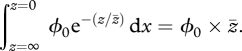2.2

A similar expression describes the distribution of CO₂ with depth, applying an analytical solution to the diffusion equation [40].

Fine roots and hyphae are assigned lengths appropriate for modern plant and mycorrhizal functional types [41,42]; these lengths and the associated characteristic depths are allowed to vary linearly as NPP deviates from modern averages for those same functional types (C₃ and C₄ grasses, and trees with any combination of deciduous or evergreen and broad or needle leaves). We can then calculate the integral of the distribution described by equation (2.2) to define the volume of the rhizosphere for the soil under 1 m² of land. Assuming a uniform distribution of soil water, we can combine this soil volume with the soil water content provided by SDGVM to get the rhizosphere solution volume. All surfaces in the rhizosphere are influenced by nutrient uptake and organic anion exudation by fine roots. Mycorrhizal fungi, on the other hand, are assumed to seek the minerals containing the most available nutrients [43], and their uptake and exudation effects are restricted to those minerals. This means that hyphal interactions with minerals are amplified in comparison with fine roots because the hyphosphere is a sub-volume of the rhizosphere.

These descriptions of nutrient uptake, exudation and carbon loss, combined with the rhizosphere and hyphosphere solution volumes, estimates of the residence time of water in micropores and rate laws of the form

2.3

allow us to calculate the alkalinity and thus the pH of the film of water on mineral surfaces [34]. In equation (2.3), the subscripts i and j refer to minerals and weathering agents a_j (H⁺, H₂O, OH⁻ and oxalate), respectively; E_app,i is the apparent activation energy for weathering mineral i; k_ij and n_ij are the rate constant and reaction order for mineral i undergoing weathering by agent a_j; R is the gas constant; and T is the temperature (K).

(c). Mineral surface area and lithology

We calculate weathering fluxes with rate laws for the silicate base-cation-bearing minerals found in basalt, granite, shale and sandstone, including feldspar and plagioclase, inosilicates, biotite and clay minerals [10]. Only silicate minerals are included; carbonates are ignored because weathering of these minerals releases CO₂ and, therefore they are less important to the long-term carbon cycle. The rate laws for H⁺, H₂O and OH⁻ are from the compendium of Palandri & Kharaka [35].

We approximate the fraction of the reactive surface area of interest for each mineral using the weight per cent of the mineral in the rock. The total reactive surface area under 1m² of land is a fixed estimate for each rock type. For basalt, we use 20 000 m² m⁻² land, the scaling value derived by Navarre-Sitchler & Brantley [44] for comparing watershed-scale weathering rates to laboratory rates on basalt substrates. Our mineralogy is that of a normal tholeittic basalt [45] and includes the Ca- and Mg-bearing minerals labradorite, augite and orthopyroxene.

For granite, we use the mineralogy of the young soils in the chronosequence examined by White et al. [46] for which we derive a total surface area of 1 788 040 m² m⁻³ soil for the silicate size fraction greater than 4 µm. Because changes in size fractions along their chronosequence indicate reaction rates four orders of magnitude lower than laboratory rates, we use a reactive silicate surface area of 179 m² m⁻³ soil. This number also compares well with the estimate of 240 m² m⁻³ soil for granite at 0 Ma by Taylor et al. [10]. The minerals providing base cations are K-feldspar, plagioclase, hornblende and biotite. We calculated global average compositions for shales and sandstones from the platform and geosynclinal averages given by Holland [47], using the same procedure he used to derive an average global sedimentary composition. The fractions of Ca, Mg, CO₂ and SO₄²⁻ indicate that 20 per cent of Ca and 66.4 per cent of Mg in sandstones is found in silicate minerals; we assumed that all of the Na and silicate Ca is in albite (Ab₉₂), all of the K is in feldspar, and the silicate Mg is in chlorite. Likewise, our shale has 28.1 per cent of its Ca and 71.9 per cent of its Mg in silicate minerals. Shales may include smectites with variable proportions of base cations; we used the composition for which Palandri & Kharaka [35] provide a rate law: K_0.04Ca_0.5(Al_2.8Fe_0.53Mg_0.7)(Si_7.65Al_0.35)O₂₀(OH)₄. We assumed that all the Na was in the same albite we used for sandstone (Ab₉₂), all the remaining silicate Ca was in smectite and all the remaining Mg in chlorite. We did not attempt to alter this mineralogy to reflect latitudinal variations in clay composition.

Brandt et al.  [48] found that the reactive surface area of chlorite corresponded to molecular steps in the t–o–t layers comprising just 0.2 per cent of the surface area determined by gas adsorption. If a shale comprised entirely clay minerals with surface areas of 0.0024 m² g⁻¹ soil and specific gravity G = 2.6, then one can calculate a surface area of 6240 m²m⁻³ soil. Because clay minerals comprise only 24 per cent and 4 per cent of our shale and sandstone, respectively, this represents a generous estimate of the reactive surface area for these rocks.

(d). Erosion and runoff corrections

Many studies have provided evidence that chemical weathering is related to physical erosion [49–54]. Montgomery & Brandon [55] suggest that erosion is related to relief. Their work in the Olympic Mountains revealed the following relationship:

2.4

where E is erosion, E₀ is background erosion due to chemical weathering (0.01 mm yr⁻¹), K = 0.00025 mm yr⁻¹ is a rate constant, R_z is the local mean relief (m) and R_c is a limiting value for relief, which we have set to 2000 m rather than 1500 m [55] to avoid numerical problems with our steepest grid points.

To incorporate the effect of relief on physical erosion, we use the standard deviation of the orography (m) as an approximation of the local mean relief for each individual grid point. Erosion values are then normalized to a mean erosion E_mean, calculated by applying equation (2.4) to the mean value of the standard deviation of orography for the world.

Following Millot et al. [53], we can calculate an approximate erosion correction to our weathering fluxes:

2.5

where i refers to the individual grid point.

A further correction is made to account for weathering responses to runoff, which may be linked to effective regolith depth. Berner [6] combined an empirical relationship between concentration and runoff:

2.6

with an approximation for the bicarbonate weathering flux at steady state:

2.7

where A is the land area being weathered and V is the volume of water in the regolith, to arrive at the following normalized correction:

2.8

where runoff₀ and runoff_t are the global runoffs at 0 Ma and time t, respectively.

Runoff is a major control on basalt weathering [56]. For a given temperature, Dessert et al. [57] noted that bicarbonate concentrations for a given temperature appear to be constant regardless of runoff, whereas bicarbonate fluxes are proportional to runoff. Although Oliva et al. [58] report that silica and cation fluxes from granite weathering may rise with increasing runoff where the mean annual temperature is greater than 13°C, concentrations decrease with increasing runoff. No simple relationship between cation fluxes and runoff is apparent for granite [53], unless physical erosion rates are high [59]. However, Amiotte-Suchet et al. [60] found that weathering rates of pure silicate sandstones and granites were about five times less responsive to runoff than pure silicate shales and basalts. As we are following the same approach assuming that these rocks comprise exclusively silicate minerals, we apply our runoff correction only to basalt and shale. We adopt the GEOCARB approach to runoff, such that the runoff for each individual grid point is normalized to the maximum runoff for the world. Our correction, therefore, either reduces weathering rates or leaves them unchanged.

By these means, we reduce the weathering contribution from low-relief regions likely to have developed thick soils that protect bedrock from further weathering [49], and we account for flushing or effective regolith depth variations on basalt and shale. With these corrections, the final weathering rate for each basalt or shale grid point is

2.9

where subscripts have the same meanings as for equation (2.3). In summary, the rate constants k_ij, reaction orders n_ij and apparent activation energies E_app,i for weathering agents a_j = H⁺, H₂O and OH⁻ operating on mineral i are from the compilation of Palandri & Kharaka [35], monthly average temperature T is generated for each grid point by HadCM3L, C_e ultimately depends on the orography data, which are boundary conditions for HadCM3L, and C_r depends on the runoff calculated by SDGVM.

3. Model validation

We used modern observational monthly temperature, humidity and precipitation datasets [61] at a resolution of 1° × 1° to drive SDGVM, producing the NPP map shown in figure 2a. Using the Water Resources eAtlas [62], we assigned grid points to world watersheds, excluding any watersheds with less than 30 per cent natural vegetation such as forest or grasslands.

Figure 2.

High-resolution modern model run. (a) Net primary production (Mg C ha⁻¹ yr⁻¹), as generated by Sheffield dynamic global vegetation model (SDGVM). Erosion (equation (2.5)) and runoff (equation (2.8)) corrections are applied to (b) annual Ca + Mg flux (log₁₀(mol Ca+Mg m⁻² yr⁻¹)) owing to weathering of silicate minerals. Corrections are multiplicative (equation (2.9)) rather than additive, so that zero flux is expected from grey grid points.

Watersheds were considered to be EM if they had at least 50 per cent forest cover comprising tree families such as Pinaceae, Fagaceae and Dipterocarpaceae, which are known to be EM [63]. Outside the watersheds, grid points were treated as EM if the trees were deciduous (such as oaks and larches) or evergreen needle-leaved (such as pines), as shown in table 1.

Table 1.

Mycorrhizal types for modern forest trees.

leaf habit	typical forest type	AM %	EM %
evergreen broadleaf	tropical rainforest	100	0
evergreen needleleaf	boreal forest	0	100
deciduous broadleaf	temperate forest	0	100
deciduous needleleaf	Larix forest	0	100

A lithology map at the same resolution was kindly supplied by Philippe Amiotte-Suchet [60]. We treated all volcanic rocks as basalt; otherwise, we used the rock types of Amiotte-Suchet et al. [60]. In a few cases, we altered the geology to match literature data. For example, the Hong watershed was entirely shale on the lithological map, even though there are igneous and metamorphic rocks in the Thao tributary contributing to the flux of cations in the river [64]. In both the Hong and Amur watersheds, we made adjustments to the lithology so that it would be similar to that of Moon et al. [64,65].

We represent most woody plants as EM except for broad-leaved evergreen trees that most closely match the tropical rainforest distribution map of Read [66]. He considered this biome to be AM with some EM. Our approach will misrepresent EM broad-leaved evergreen dipterocarps and oaks as AM, and could wrongly treat important Late Cretaceous AM needle-leaved trees such as Sequoia [67] as EM.

(a). Observed and predicted watershed Ca + Mg weathering fluxes

We compared our simulated weathering fluxes of Ca + Mg at the catchment scale with measurements reported in a global compendium [28] in which 29 watersheds fit the criteria for at least 30 per cent natural vegetation outlined above (figure 3). These watersheds are in Africa, Asia, North and South America and Australia, and contain a range of vegetation types as the dominant land cover, including boreal, temperate and tropical forests. Overall, following the application of erosion and runoff corrections, our predicted fluxes show close correspondence with the measurements reported by Gaillardet et al. [28] for watersheds producing high Ca + Mg fluxes (R² = 0.726 for untransformed data). A linear fit comparing modelled and observed log-transformed fluxes has a slope of 0.913; the slope would be 1.0 for a perfect match (figure 3e). The spread of the predictions at the lower end of the scale, however, suggests that the rocks undergoing weathering in these watersheds are not captured by the 1° × 1° lithology map of Amiotte-Suchet et al. [60] or that our erosion and runoff corrections do not capture smaller scale variations in Ca + Mg flux from silicate weathering. These results are obtained with an input climate averaged over 11 years (1992–2002). We also tested a HadCM3L climate for the modern day that gives a slope of 0.732 for log-transformed data. However, R² for the untransformed data is only 0.5 for this model run, because the observed Fly River (Papua New Guinea) runoff is over six times larger than that produced by HadCM3L.

Figure 3.

Watershed comparison of high-resolution model output with literature data after Gaillardet et al. [28]. We used observational data [61] in (a,c,e) and HadCM3L output in (b,d,f) to force the SDGVM and weathering modules. Model results are shown for individual watersheds with no corrections (a,b), with erosion correction only (c,d) and with erosion and runoff corrections (e,f) applied as stipulated in the text. The dominant mycorrhizal functional type of the watersheds is either AM (open circles) or EM (filled circles). Lines fitted to data are dashed, whereas hypothetical one-to-one lines are dotted. Ideally, these two lines should match.

These model-data comparisons serve to verify our modelling approach at the catchment scale, despite a number of simplifying assumptions, such as uniform soil type and depth, lithology and mineralogy. It further indicates that our numerical representation of biological and abiotic weathering processes are probably realistic and therefore have some utility when extrapolated into the past. This view is supported by the similarity between our Ca + Mg flux modelled for the Orinoco watershed in South America (0.056 mol Ca + Mg m⁻² yr⁻¹) with that obtained from a more detailed multi-layered soil chemistry model (0.045 mol Ca + Mg m⁻² yr⁻¹) for the same catchment that includes a treatment of the precipitation of secondary clay minerals, the inhibiting action of aluminium on weathering rates and trace quantities of calcite in silicate rocks [25].

Because our model simulates seasonal cycles in biology and climate, calculated monthly Ca and Mg weathering fluxes can be compared with observed seasonal fluctuations. In the Hong watershed (figure 4) that lies within China and Vietnam, our simulated seasonal amplitude is similar to observations reported by Moon et al. [64] showing warmer summers are associated with doubling the weathering fluxes compared with those in the wintertime. It is important to appreciate that modelled catchment scale estimates of cationic weathering fluxes in figure 4 are the mean of multiple grid points with tropical to subtropical climates. Therefore, we explored how our modelled variability compares with observations made under the contrasting conditions of temperate to boreal forest in the Amur watershed in Mongolia [65]. Overall, the comparison shows that the spatial variability of our cationic fluxes is comparable with observations for this watershed.

Figure 4.

Model runs compared with data for individual watersheds. The model outputs are corrected for erosion and runoff. The mean (solid black circles) and standard deviation (error bars) of the modelled cationic fluxes from silicate weathering for grid points within the watersheds are shown for comparison with the observational data (squares). (a) Hong river. Original observational data from near the mouth of the river [64] show seasonal differences in fluxes that our model captures. (b) Amur river. Silicate weathering rates, calculated using mean annual runoff [65], were divided by 12 to give monthly average values. The lowest four points are from sample sites on the main Amur channel.

(b). Global continental weathering

We next extend our simulations of terrestrial NPP and continental Ca + Mg fluxes to the global scale (figure 2b). Comparison of the two global maps indicates a general correspondence between areas of high productivity and high weathering rates, but these rates are also linked to the underlying lithology; regions with the highest weathering fluxes of less than 0.4 mol m⁻² yr⁻¹ typically coincide with the location of basalt.

At the global scale, little is known about the spatial extent of highly active weathering regions, making validation of our global weathering map difficult. Hartmann et al. [17] published a global map of CO₂ consumption on a 1° × 1° grid resolution based on applying a spatially explicit function for CO₂ consumption by weathering of silicate and carbonate rocks. Our weathering map is not directly comparable with that of Hartmann et al. [17], which accounts for the weathering of all rock types, including carbonates. Our measure of silicate weathering is the flux of Ca + Mg, which we do not translate into CO₂ consumption. Nevertheless, both maps show regions of agreement. In particular, the locations of high CO₂ consumption by chemical weathering in the tropical forests of South America, central Africa and throughout South East Asia correspond to our high rates of weathering (figure 2b). Our erosion correction indicates low fluxes for large parts of the northern hemisphere, whereas our runoff correction sharply reduces the flux from the Siberian, Ethiopian and Deccan Traps. We also come to a similar conclusion that weathering hotspots produce the bulk of the global weathering flux. Our results indicate that 10 per cent of the silicate land area of 106 Tm² in our map produces 66 per cent of the Ca + Mg flux from silicate weathering. This is higher that the figures given by Hartmann et al. [17], where 9 per cent of the global exorheic area of 121 Tm² produces 50 per cent of the CO₂ consumption. In our case, hotspots occur where relief, runoff and NPP are high, especially on basalt, and it is therefore instructive to investigate the effect of lithology. For an all-granite world of total area 127 Tm², our model produces 41 per cent of global Ca + Mg from 12.7 Tm², or 60 per cent of global Ca + Mg from 20 per cent of the land area. Such a world is less influenced by hotspots than expected by Hartmann et al. [17], and because granites produce more Ca and Mg than sandstones and shales, we get a higher global Ca + Mg flux of 5.20 mol m⁻² yr⁻¹. This is closer to some global literature estimates [3,68] but far in excess of estimates for igneous rocks alone (table 2). Furthermore, Dessert et al. [56,57] expected the contribution of basalts to global CO₂ consumption to be non-negligible because they weather 5–10 times faster than granite and gneiss. For the 47 grid points on the Deccan Traps, the ratio of the weathering rates for the standard and all-granite runs had a mean of 2.9 and a maximum of 9, with six grid points within the range 5–10 estimated by Dessert et al. [56,57]. Worldwide, our basalt–granite weathering ratio has a mean of 4.9, in line with that reported by Dessert et al. [56,57].

Table 2.

Modern Ca and Mg fluxes from silicate weathering. Values are in Tmol Ca+Mg yr⁻¹. bas, basalt; gr, granite; sed, sedimentary.

basalt	granite	bas + gr	sed	total	reference	remarks
20.74	4.00	24.74	2.59	27.34	this study, observed climate	uncorrected
8.92	1.57	10.50	0.97	11.47	this study, observed climate	erosion correction
1.68	1.57	3.26	0.51	3.77	this study, observed climate	erosion and runoff corrections
16.04	3.71	19.75	2.66	22.41	this study, GCM climate	uncorrected
8.97	1.80	10.77	1.21	11.98	this study, GCM climate	erosion correction
1.90	1.80	3.71	0.68	4.39	this study, GCM climate	erosion and runoff corrections
0	13.28	13.28	0	13.28	this study, granite world	uncorrected
0	5.20	5.20	0	5.20	this study, granite world	erosion correction
0	5.20	5.20	0	5.20	this study, granite world	erosion and runoff corrections
		2.50			Gaillardet et al. [28]	from their table 3. The authors note that their CO2 consumption flux is 40% lower than that of Berner et al. [3]
		0.92		5.36	Meybeck [68]	column 3 comprises granite, gabbro, gneiss, mica-schists, and volcanic rocks from his table 5
		1.67		6.11	Meybeck [68]	as above but including ‘mixed metamorphic’ (serpentinite, marble, amphibolite, etc.) from his table 5
		2.8	3.1	5.9	Berner et al. [3]	uses global average river data

A further approach to validation is possible by comparing our global continental fluxes with earlier published estimates based on elemental ratios and monolithological watershed data to estimate the silicate contribution of solutes to river water (table 2). Global totals are similar whether the model is driven by observations of modern climatology or with the HadCM3L simulated modern climate (table 2). Simulated global weathering of granite and basalt (i.e. igneous) silicate rocks are comparable with estimates published by Hartmann et al. [28] and Meybeck [68], after corrections owing to erosion and runoff, as applicable. Strontium isotope data have been interpreted to suggest a present-day basalt flux that is ca 44 per cent [69] or 35 per cent [70] of the total, in agreement with Dessert et al. [56] who estimated the contribution of basalt weathering to global silicate CO₂ consumption to be ca 35 per cent. Our results are in agreement with these studies (table 2), with basalt weathering being 45 per cent of the total (table 2).

Our modern flux of 3.77 Tmol Ca + Mg yr⁻¹ implies a CO₂ consumption flux owing to the weathering of Ca and Mg silicates of 7.54 Tmol C yr⁻¹ (table 2), which is comparable with the estimate of 7.1 Tmol C yr⁻¹ given by Gaillardet et al. [28]. The CO₂ consumption flux from basalt reported by Hartmann et al. [17] (3.55 Tmol C yr⁻¹) provides an upper limit to the flux of Ca and Mg from basalt of 1.78 Tmol Ca + Mg yr⁻¹, if one assumes that all of the bicarbonate is balanced by Ca and Mg, which again supports our estimate of 1.68 Tmol Ca + Mg yr⁻¹ (table 2).

There are few global estimates of silicate Ca + Mg fluxes from sedimentary rocks (shales and sandstones). Berner et al. [3] calculated global weathering rates using riverine data of Meybeck [71] and the assumption that 15 per cent of calcium in all sediments globally is found in silicate minerals [47]. However, this approach gives numbers that are about an order of magnitude larger than our estimated weathering of sedimentary rocks (following erosion and runoff corrections), in spite of our using similar mineralogies for sandstones and shales (table 2). We also employed a very high mineral surface area for these rocks, but the minerals (albite, K-feldspar, chlorite and smectite) have relatively slow weathering rate laws [35]. Without any corrections owing to erosion or runoff, we obtain for these rocks a flux similar to that of Berner et al. [3]. However, we can see no rationale for excluding the effects of erosion and runoff because this would imply that the weathering front on shales and sandstones is never obstructed by thick soils or other occlusions, and that these rocks do not respond to the exposure of fresh surfaces following physical erosion.

4. Present-day weathering by plants and mycorrhizal fungi

As expected from a weathering model driven by the biological proton cycle [16], our simulations reveal strong relationships between vegetation NPP and the flux of Ca and Mg owing to the weathering of silicate rocks [10]. These relationships vary with lithology and plant and mycorrhizal functional type (figure 5). Because the runoff and erosion corrections (equations (2.5) and (2.8)) account for changes in soil properties such as reacting mineral surface area rather than characteristics of the plants or their symbionts, we analyse the potential (uncorrected) flux of Ca + Mg from our weathering model.

Figure 5.

Uncorrected Ca + Mg fluxes from weathering of (a,b) basalt and (c,d) granite versus net primary productivity for the high-resolution modern model run, showing plant (a,c) and mycorrhizal (b,d) functional types. Watersheds that have at least 30% natural grasslands or forest according to the Water Resources eAtlas [62] have been assigned a mycorrhizal type based on the dominant plant families. African and South American watersheds are all considered to be AM. Pixels outside the Water Resources eAtlas watersheds were assigned a mycorrhizal type based on plant functional type, as shown in table 1.

As expected from geochemical theory [72] and field observations [56], basalt weathers faster than granite. In the model, this occurs for two reasons. First, because the reactive mineral surface area of basalt is two orders of magnitude higher than granite, and second, because the rate laws for dissolution of minerals of basalt are faster than those of granite (figure 5). However, the higher buffering capacity of basalt compared with granite limits the effect of acidification on its weathering rates. This means that on basalt, acidification by EM fungi is primarily important at low NPP. On granite, the ability of EM fungi to focus protons on minerals makes them more effective weathering agents than AM fungi as NPP increases.

The gradient in NPP at the global scale (figure 2a) is driven primarily by climate linked to vegetation type. Evergreen broad-leaved trees (i.e. tropical rainforests) have the highest NPP of all the simulated PFTs, and they drive the highest weathering fluxes on both rock types (figure 5a,c). Deciduous broad-leaved trees (i.e. temperate forests) are the next most productive, and needle-leaved trees of boreal forests are generally less productive again. In terms of weathering, evergreen broad-leaved trees achieved high rates, even though they are usually AM, because of high productivity driving the biological proton cycle and high acidity of the soil solution.

Deciduous broad-leaved trees often produce lower Ca + Mg fluxes than needle-leaved trees of the same or even lower NPP that occupy cooler climates on basalt. This effect does not occur if all trees are considered to be AM. On granite, all EM trees except for evergreen broad-leaved trees produce Ca + Mg fluxes as a linear function of NPP, and these fluxes are higher than those of AM trees.

The fractional contribution of each plant and mycorrhizal functional type to the global weathered flux of Ca + Mg is given in table 3, which indicates that although they contribute only 46 per cent of global NPP and cover 19 per cent of global land area, evergreen broad-leaved trees contribute 72 per cent of the Ca + Mg flux from silicate weathering. Most of these trees are treated as AM, so a similarly high fraction of the global Ca + Mg flux is due to AM fungi. These results indicate that this PFT is the single most important agent of biological weathering, with mycorrhizal functional type being of secondary importance.

Table 3.

Contributions of functional types to global weathering.

	area	fraction of	corrected flux	fraction of	NPP	fraction of
functional type	(Tm2)	total area	(Tmol yr−1)	global flux	(Pg C yr−1)	global NPP
bare	23.5	0.185	0	0	0	0
C3 grass	8.7	0.069	0.089	0.024	1.278	0.020
C4 grass	13.7	0.108	0.205	0.054	4.925	0.079
Evg broad	24.2	0.191	2.173	0.577	28.506	0.456
Evg needle	23.7	0.186	0.243	0.065	7.199	0.115
Dec broad	28.3	0.223	1.025	0.272	19.594	0.313
Dec needle	4.8	0.038	0.029	0.008	1.015	0.016
all plants	103.4	1.000	3.765	1.000	62.517	1.000
AM fungi	70.7	0.683	2.815	0.748	48.898	0.782
EM fungi	32.8	0.317	0.950	0.252	13.619	0.218

One of the 12 testable hypotheses on the geobiology of weathering [73] is that the location and extent of biological weathering is controlled by carbon fixation [15,43]. Our model is designed so that biological weathering depends on NPP, but at the global scale, weathering is enhanced at different rates depending on rock type and on plant and mycorrhizal functional types. Comparison of the maps in figure 2 indicates that global NPP maps cannot be used to identify the locations producing the highest silicate weathering fluxes owing to the strong influence of lithology, erosion and runoff. The enhancement of silicate weathering by EM fungi compared with AM fungi is attenuated for the most productive trees on the rocks rich in Ca and Mg. Therefore, figure 5 shows that the hypothesized positive relationship between NPP and biological weathering [15] is strongly mediated by plant and mycorrhizal functional type acting in concert with abiotic factors.

5. Weathering in the past

(a). Palaeolithology

Because of the lack of lithological maps for the time intervals corresponding to the suite of HadCM3L palaeoclimate simulations required for continental weathering calculations, we developed our own, starting with entirely granite worlds and adding other rock types by hand. Granite was replaced with flood basalts of appropriate age and size based on published data concerning large igneous provinces [74–78] and websites hosted by the universities of Leicester (http://www.le.ac.uk/gl/ads/SiberianTraps/Index.html) and Bristol (http://palaeo.gly.bris.ac.uk/Palaeofiles/Permian/SiberianTraps.html). Emplacement of the Deccan Traps occurred near the K/T boundary [78] just after the date of our Maastrichtian run (67 Ma). We have included them in our weathering calculations, and they comprise an important weathering hotspot at this time, and also in the Eocene.

Using the online maps produced by the United States Geological Survey and the Atlas of Mesozoic and Cenozoic Coastlines [79], we replaced other granitic regions with limestones, shales and sandstones of appropriate age. We attempted to locate sedimentary basins using the available boundary conditions (orography and its standard deviation), seeking simple rules for the probable locations of terrestrially derived sandstones and shales based on their modern distributions [60]. Overall, the lithology of 40–50% of the continental grid points could be predicted by assuming shale for orography under 200 m and standard deviation under 600 m, and sandstone for orography between 200 and 1300 m and standard deviation under 100 m. This approach is distinct from previous attempts to model global continental weathering over geological time, which assumed all grid points contained all rock types in their modern global proportions [20]. However, we aimed to capture the effect of basalt weathering with respect to changes in basalt production and erosion over geological time, as well as palaeogeography and palaeoclimate.

In spite of adding sediments at the expense of granite to generate palaeolithologies, overall land areas underlain by granite were higher than those of Bluth & Kump [80]. However, the latter are known to be underestimated owing both to lack of data about older lithofacies and inability to account for erosion of rock units  [18]. Gibbs & Kump [81] revised the Bluth & Kump modern lithological map, but over one-quarter of their land area is assigned to ‘fold belts’ rather than being included in the lithological categories of Amiotte-Suchet et al. [60], so their total areas for many of our rock types are lower than ours. We recognize the limitations inherent in this approach to generating lithologial maps for weathering calculations, but the advantages are that it establishes a standardized method for exploring how continental weathering may have changed over geological time. Nevertheless, our estimates of continental weathering should be regarded as exploratory rather than definitive at this stage.

(b). Global patterns of terrestrial vegetation productivity and weathering in the past

Global patterns of terrestrial NPP over geological time vary with latitude, climate, atmospheric CO₂ concentration and continental configuration (figure 6). In particular, areas of highest NPP are sustained in the tropics with year-round warmth, high precipitation and high solar energy. Global terrestrial NPP has varied considerably over geological time (figure 6), and functions to account for changes in weathering by plants under different CO₂ and climate have been included in models of the long-term carbon cycle [5,8]. Taylor et al. [10] compared these functions with the estimates that were produced using SDGVM. Total NPP for our time slices compares well with earlier SDGVM estimates of Beerling & Woodward [22] and with functions developed by Volk [12] and Bergman et al. [8], but is considerably higher than that of Berner [5] when these functions are scaled by modern NPP.

Figure 6.

NPP for several timeslices in the (a,b) Cenozoic and (c–g) Mesozoic.

Comparison of global patterns of NPP and weathering in the past serves to reinforce the idea that there is not always a one-to-one correspondence between the two (figures 6 and 7). For example, in the Late Triassic (Norian), although NPP is highest in the evergreen broad-leaved forests around the south-eastern coast of Asia, the highest Ca + Mg fluxes are associated with deciduous broad-leaved trees on the southern Siberian Traps. In the Jurassic (Kimmeridgian), the highest Ca + Mg fluxes occur on the Ferrar (Antarctica and Australia) and Karoo (southern Africa and Antarctica) basaltic regions under herbaceous vegetation, and on the Central Atlantic Magmatic Province (CAMP) basalts under evergreen broad-leaved forests. These sites are not coincident with global maximum NPP associated with evergreen broad-leaved forests on granites of Southeast Asia and Central America. The low runoff simulated over most of the CAMP basalts and the Siberian Traps means that these regions do not contribute as much Ca and Mg to rivers as might have been expected, given their large area and the equatorial position of CAMP.

Figure 7.

Ca + Mg fluxes for several timeslices in the (a,b) Cenozoic and (c–g) Mesozoic.

Other attempts to model weathering in the Triassic have focused on the Carnian and Rhaetian just before and just after the Norian, respectively. Our global weathering pattern (figure 7g) differs substantially from the CO₂ consumption maps of Goddéris et al.  [82], where the highest weathering occurs in the equatorial region. Despite high temperatures and adequate moisture to support deciduous broad-leaved trees at the equator, we have no equatorial weathering hotspots in the Norian because most of the rocks are either granite or sedimentary.

Cretaceous simulations indicate that the CAMP basalts produce the highest weathering fluxes in the Aptian (119 Ma), where they coincide with high runoff and high NPP of broad-leaved evergreen forest. This contrasts with the situation in the Cenomanian, where these rocks are associated with low runoff and sparse forest coverage. The weathering map for the Cenomanian bears some similarity to the CO₂ consumption maps of Goddéris et al. [82]. Our map shows a greater proportion of flux from Antarctica, which was forested with evergreen needle-leaved trees in general agreement with fossil evidence [67]. Runoff on the CAMP basalts was low and the remainder of equatorial Africa was not underlain by basalt; so equatorial Africa was not a weathering hotspot despite the high NPP and high predicted CO₂ consumption in the simulations of Goddéris et al. [82]. Instead, the highest fluxes of the Cenomanian come from AM evergreen broad-leaved forests of the wet Emeishan (China) basalts, followed by EM deciduous broad-leaved and evergreen needle-leaved trees on the somewhat drier and cooler Karoo and Siberian Traps basalts, respectively. EM trees dominate 70 per cent of the basalt grid points in the Cenomanian, in agreement with Taylor et al. [10], but this is not the case in the latest Maastrichtian when the CAMP and Deccan Trap basalts are covered with high-NPP AM evergreen broad-leaved trees.

(c). Biological weathering on the continents over geological time

For each time step, we undertook three simulations to enable us to investigate and isolate the changing role of vegetation, mycorrhiza and climate on continental weathering rates over geological time: (i) a standard run with mycorrhizal functional type allocated to trees according to table 1 (all AM in the Aptian, Kimmeridgian and Norian); (ii) a non-mycorrhizal run, with only fine roots directly impacting soil chemistry; and (iii) a run with no impact of roots or fungal hyphae on soil chemistry. The latter ‘no vegetation’ run still includes the soil water content and runoff from SDGVM. The net direct effect of land plants on chemical weathering is calculated as the difference between the total global Ca + Mg fluxes for the mycorrhizal and ‘no vegetation’ cases. Results, along with the atmospheric CO₂ used to force the models, are shown in table 4.

Table 4.

Ca and Mg fluxes from silicate weathering. Values are in Tmol Ca+Mg yr⁻¹. bas, basalt; gr, granite; sed, sedimentary.

basalt	granite	bas + gr	sed	total	CO2 (ppm)	time (Ma)	period
2.252	6.237	8.489	1.427	9.916	1116	216	Norian
0.933	2.927	3.860	0.774	4.634	1120	153	Kimmeridgian
7.910	3.931	11.841	0.936	12.777	1120	119	Aptian
7.800	4.856	12.656	1.057	13.713	1378	95	Cenomanian
7.707	10.519	18.226	0.592	18.818	838	67	Maastrichtian
7.021	3.728	10.749	1.152	11.901	560	55	Eocene
1.769	1.706	3.475	0.650	4.125	280	0	preindustrial

Figure 8a indicates the potential for up to fourfold variations in continental weathering over the past 220 Myr relative to the present day (table 4). These absolute global fluxes obtained from our process-based modelling are of the same order of magnitude as those obtained with global geochemical models using independent methodologies [8,9,29], but are often higher, as shown in figure 8a. According to the above sensitivity analyses, climate dominates global weathering reflecting the strong temperature control on rate laws of mineral dissolution (figure 8b,c). The exceptions to this pattern are the Late Triassic (Norian, 216 Ma) and Early Jurassic (Kimmeridgian, 153 Ma) simulations, which show unusually low weathering regimes, given the warm average land surface temperatures. In these two cases, the continental configuration of land masses created a supercontinent with extensive deserts and a more arid environment (figure 8c), causing low soil water content and runoff that hinders chemical weathering.

Figure 8.

Global weathering and climate for several timeslices. (a) Total annual silicate weathering flux of Ca + Mg. (b) Contribution of climate, roots and mycorrhizal fungi to silicate weathering fluxes of Ca + Mg. (c) Global mean annual temperature (MAT) and precipitation (MAP). (d) The weathering efficiency of plants (f_E) normalized using our modern flux and that of Berner [5,9]. The f_E values used in the most recent GEOCARB models [7,9] are shown for comparison.

According to our modelling, vegetation enhances weathering over and above that caused by climate in all simulations, in agreement with numerous field studies [15,83] (figure 8a,b). For the contemporary climate and CO₂ (i.e. 0 Ma), mycorrhizal vegetation increases continental weathering by a factor of 1.3 at the global scale, and the same set of simulations afford a further opportunity for independent validation against observations. On Icelandic basalt at 0 Ma, this ratio increases to 2.8 for sites dominated by deciduous broad-leaved trees, and 1.9 for those with evergreen needle-leaved trees. These numbers are slightly low when compared with estimates of three to four derived for adjacent-vegetated and non-vegetated catchments in Iceland [84]. Moulton et al. [84] did not find a significant difference between deciduous broad-leaved trees (Betula pubescens) and evergreen needle-leaved trees (Picea spp., Abies spp.), although they note that the B. pubescens trees were stunted.

In the Norian (216 Ma), Kimmeridgian (153 Ma) and Aptian (119 Ma), mycorrhizal fungi exert a minor additional effect on biological weathering because they are exclusively modelled to be the ancestral AM type that predominated prior to the later evolution of EM fungi. AM fungi are thought to be less effective than EM fungi because they enhance rather than replace the nutrient uptake functions of fine roots, and because they do not tend to exude organic acids [15].

In all simulations, after and including the Cenomanian, the boreal and temperate forests are assigned EM fungal partnerships following the function of Taylor et al. [10] that characterized the sigmoidal rise in EM vegetation at weathering hotspots during the Cretaceous [10]. This function has 0.1 per cent EM vegetation at weathering hotspots at the estimated time of EM origination (180 Ma) according to molecular data [15,85], rising to 71 per cent at 95 Ma. As a result of the ability of these fungi to target nutrient-bearing minerals, EM and AM fungi together contribute as much as or more than the amount of weathering driven by vegetation alone (figure 8b). In the Cenomanian, mycorrhizal fungi exert an especially large effect (figure 8a,b), and EM vegetation is found on 70 per cent of basalt grid points, including the Karoo and Siberian Traps as described above, of which more than 40 per cent is provided owing to fungal activities (figure 8b and table 4). These global-scale simulations provide new support for the idea previously proposed by Taylor et al. [15]: the rise of EM trees may have contributed to the CO₂ drawdown previously attributed to the spread of angiosperms since the Mid- to Late Cretaceous. From these results, we can create a new dimensionless plant weathering efficiency function (f_E) to better characterize how terrestrial ecosystem weathering changed over geological time (figure 8d). The resulting pattern shows that terrestrial ecosystem weathering could have been up to four to five times more efficient in the past relative to today, especially during times of global warmth, high CO₂ and extensive land cover by EM vegetation. The pattern of ecosystem weathering efficiency over the past 215 Myr differs substantially from the f_E function included in geochemical models [7,8], which is between 0.875 and 1.0 for the past 250 Myr. Because f_E is normalized to the present-day flux, our values exceed one in the Cretaceous. One possible explanation for such unexpectedly strong plant effects is that the CO₂ fertilization function of the GEOCARB models does not adequately account for the significantly higher global NPP of the Cretaceous. Cenomanian global NPP (138 Pg C yr⁻¹) is more than twice as high as it is today (62 Pg C yr⁻¹).

6. Concluding remarks

Our global modelling strategy is well-validated against modern observations at the catchment and global scales and, therefore, appears to be robust, at least for the present-day situation (figures 3,4 and table 2). For contemporary ecosystems, our simulations indicate that the mycorrhizal status of trees has an effect on spatially resolved Ca + Mg fluxes from silicate weathering. The more ‘aggressive’ EM fungi do not necessarily produce higher fluxes if the trees have high NPP and are weathering basalt (figure 5). For NPP under 10 Mg C ha⁻¹ yr⁻¹, EM fungi enhance weathering compared to AM fungi (figure 5). Fine roots and hyphae enhance weathering fluxes of Ca and Mg by a factor of 1.2–2.1, and the highest fluxes occur where NPP is the highest for a given rock type. Mycorrhizal functional type is however less important to global weathering fluxes than PFT in the modern world.

When extrapolated back into the past, the same modelling approach indicates the potential for major enhancement of weathering by terrestrial ecosystems, with the coevolution of ectomycorrhizas and vegetation being an especially important factor (figure 8 and table 4). The enhancement is greater than previously suggested by empirical functions [7] with implications for the role of the evolving biota in regulating the global atmospheric CO₂ concentration. One of the major differences between this study and previous studies of the effect of plants on the long-term geochemical carbon cycle [7–10,20] is that we present fluxes (tables 2–4; figures  2b, 3–5, 7 and 8) that have been calculated without calibration to any assumed or observed weathering rate or degassing flux. Our model could be calibrated by changing the reactive mineral surface area for each rock type until our modern flux matched that of Gaillardet et al. [28], for example. Such a calibration is probably necessary if we were to use our model to generate revised estimates of CO₂ drawdown to produce a new CO₂ curve, because our uncalibrated fluxes could cause unrealistic CO₂ drawdown.

In conclusion, this study demonstrates ‘proof of concept’ by reporting novel approaches for the more realistic process-based treatment of plant–fungal interactions with the geosphere at the global scale. Accurately capturing such interactions is critical for better understanding the coevolution of terrestrial ecosystems, CO₂ and climate over geological time, and constitutes a first step towards developing ‘next-generation’ geochemical models incorporating the effects of mycorrhizal evolution.

References

- 1.Ebelmen J. 1845. Sur les produits de la decomposition des especes minerales de la famille des silicates. Annales des Mines 7, 3–66 [Google Scholar]
- 2.Urey H. 1952. The planets, their origin and development. New Haven, CT: Yale University Press [Google Scholar]
- 3.Berner R., Lasaga A., Garrels R. 1983. The carbonate–silicate geochemical cycle and its effect on atmospheric carbon dioxide over the past 100 million years. Am. J. Sci. 283, 641–683 10.2475/ajs.283.7.641 (doi:10.2475/ajs.283.7.641) [DOI] [PubMed] [Google Scholar]
- 4.Holland H. 1984. The chemical evolution of the atmosphere and oceans. Princeton, NJ: Princeton University Press [Google Scholar]
- 5.Berner R. 1991. A model for atmospheric CO2 over Phanerozoic time. Am. J. Sci. 291, 339–376 10.2475/ajs.291.4.339 (doi:10.2475/ajs.291.4.339) [DOI] [PubMed] [Google Scholar]
- 6.Berner R. 1994. GEOCARB II: a revised model of atmospheric CO2 over Phanerozoic time. Am. J. Sci. 294, 56–91 10.2475/ajs.294.1.56 (doi:10.2475/ajs.294.1.56) [DOI] [Google Scholar]
- 7.Berner R., Kothavala Z. 2001. Geocarb III: a revised model of atmospheric CO2 over Phanerozoic time. Am. J. Sci. 301, 182–204 10.2475/ajs.301.2.182 (doi:10.2475/ajs.301.2.182) [DOI] [Google Scholar]
- 8.Bergman N., Lenton T., Watson A. 2004. COPSE: a new model of biogeochemical cycling over Phanerozoic time. Am. J. Sci. 304, 397–437 (doi:10.2475/ajs.304.5.397) [Google Scholar]
- 9.Berner R. 2006. GEOCARBSULF: a combined model for Phanerozoic atmospheric O2 and CO2. Geochim. Cosmochim. Acta 70, 5653–5664 10.1016/j.gca.2005.11.032 (doi:10.1016/j.gca.2005.11.032) [DOI] [Google Scholar]
- 10.Taylor L., Banwart S., Leake J., Beerling D. 2011. Modelling the evolutionary rise of the ectomycorrhiza on subsurface weathering environments and the geochemical carbon cycle. Am. J. Sci. 311, 369–403 10.2475/05.2011.01 (doi:10.2475/05.2011.01) [DOI] [Google Scholar]
- 11.Walker J., Hays P., Kasting J. 1981. A negative feedback mechanism for the long-term stabilization of the Earth's surface temperature. J. Geophys. Res. 86, 9776–9782 10.1029/JC086iC10p09776 (doi:10.1029/JC086iC10p09776) [DOI] [Google Scholar]
- 12.Volk T. 1987. Feedbacks between weathering and atmospheric CO2 over the last 100 million years. Am. J. Sci. 287, 763–779 10.2475/ajs.287.8.763 (doi:10.2475/ajs.287.8.763) [DOI] [Google Scholar]
- 13.Knoll M., James W. 1987. Effect of the advent and diversification of vascular land plants on mineral weathering through geologic time. Geology 15, 1099–1102 10.1130/0091-7613(1987)15%3C1099:EOTAAD%3E2.0.CO;2 (doi:10.1130/0091-7613(1987)15〈1099:EOTAAD〉2.0.CO;2) [DOI] [Google Scholar]
- 14.Berner R. 1992. Weathering, plants, and the long-term carbon cycle. Geochim. Cosmochim. Acta 56, 3225–3231 10.1016/0016-7037(92)90300-8 (doi:10.1016/0016-7037(92)90300-8) [DOI] [Google Scholar]
- 15.Taylor L., Leake J., Quirk J., Hardy K., Banwart S., Beerling D. 2009. Biological weathering and the long-term carbon cycle: integrating mycorrhizal evolution and function into the current paradigm. Geobiology 7, 171–191 10.1111/j.1472-4669.2009.00194.x (doi:10.1111/j.1472-4669.2009.00194.x) [DOI] [PubMed] [Google Scholar]
- 16.Banwart S. A., Berg A., Beerling D. J. 2009. Process-based modeling of silicate mineral weathering responses to increasing atmospheric CO2 and climate change. Glob. Biogeochem. Cycles 23, GB4013. 10.1029/2008GB003243 (doi:10.1029/2008GB003243) [DOI] [Google Scholar]
- 17.Hartmann J., Jansen N., Dürr H., Kempe S., Köhler P. 2009. Global CO2-consumption by chemical weathering: what is the contribution of highly active weathering regions? Glob. Planet. Change 69, 185–194 10.1016/j.gloplacha.2009.07.007 (doi:10.1016/j.gloplacha.2009.07.007) [DOI] [Google Scholar]
- 18.Gibbs M., Bluth G., Fawcett P., Kump L. 1999. Global chemical erosion over the last 250 Myr: variations due to changes in paleogeography, paleoclimate, and paleogeology. Am. J. Sci. 299, 611–651 10.2475/ajs.299.7-9.611 (doi:10.2475/ajs.299.7-9.611) [DOI] [Google Scholar]
- 19.Goddéris Y., Joachimski M. 2004. Global change in the Late Devonian: modelling the Frasnian–Famennian short-term carbon isotope excursions. Palaeogeogr. Palaeoclimatol. Palaeoecol. 202, 309–329 10.1016/S0031-0182(03)00641-2 (doi:10.1016/S0031-0182(03)00641-2) [DOI] [Google Scholar]
- 20.Donnadieu Y., Goddéris Y., Pierrehumbert R., Dromart G., Fluteau F., Jacob R. 2006. A GEOCLIM simulation of climatic and biogeochemical consequences of Pangea breakup. Geochem. Geophys. Geosyst. 7, 1019. 10.1029/2006GC001278 (doi:10.1029/2006GC001278) [DOI] [Google Scholar]
- 21.Goddéris Y., Donnadieu Y., de Vargas C., Pierrehumbert R., Dromart G., van de Schootbrugge B. 2008. Causal or casual link between the rise of nanoplankton calcification and a tectonically-driven massive decrease in Late Triassic atmospheric CO2? Earth Planet. Sci. Lett. 267, 247–255 10.1016/j.epsl.2007.11.051 (doi:10.1016/j.epsl.2007.11.051) [DOI] [Google Scholar]
- 22.Beerling D., Woodward F. 2001. Vegetation and the terrestrial carbon cycle: modelling the first 400 million years. Cambridge, UK: Cambridge University Press [Google Scholar]
- 23.Gordon C., Cooper C., Senior C., Banks H., Gregory J., Johns T., Mitchell J., Wood R. 2000. The simulation of SST, sea ice extents and ocean heat transports in a version of the Hadley Centre coupled model without flux adjustments. Clim. Dyn. 16, 147–168 10.1007/s003820050010 (doi:10.1007/s003820050010) [DOI] [Google Scholar]
- 24.Pope V., Gallani M., Rowntree P., Stratton R. 2000. The impact of new physical parametrizations in the Hadley Centre climate model: HadAM3. Clim. Dyn. 16, 123–146 10.1007/s003820050009 (doi:10.1007/s003820050009) [DOI] [Google Scholar]
- 25.Roelandt C., Goddéris Y., Bonnet M. 2010. Coupled modeling of biospheric and chemical weathering processes at the continental scale. Glob. Biogeochem. Cycles 24, GB2004. 10.1029/2008GB003420 (doi:10.1029/2008GB003420) [DOI] [Google Scholar]
- 26.Goddéris Y., François L., Probst A., Schott J., Moncoulon D., Labat D., Viville D. 2006. Modelling weathering processes at the catchment scale: The WITCH numerical model. Geochim. Cosmochim. Acta 70, 1128–1147 10.1016/j.gca.2005.11.018 (doi:10.1016/j.gca.2005.11.018) [DOI] [Google Scholar]
- 27.Donnadieu Y., Goddéris Y., Bouttes N. 2009. Exploring the climatic impact of the continental vegetation on the Mezosoic atmospheric CO2 and climate history. Clim. Past 5, 85–96 10.5194/cp-5-85-2009 (doi:10.5194/cp-5-85-2009) [DOI] [Google Scholar]
- 28.Gaillardet J., Dupré B., Louvat P., Allegre C. 1999. Global silicate weathering and CO2 consumption rates deduced from the chemistry of large rivers. Chem. Geol. 159, 3–30 10.1016/S0009-2541(99)00031-5 (doi:10.1016/S0009-2541(99)00031-5) [DOI] [Google Scholar]
- 29.Wallmann K. 2001. Controls on the Cretaceous and Cenozoic evolution of seawater composition, atmospheric CO2 and climate. Geochim. Cosmochim. Acta 65, 3005–3025 10.1016/S0016-7037(01)00638-X (doi:10.1016/S0016-7037(01)00638-X) [DOI] [Google Scholar]
- 30.Markwick P., Valdes P. 2004. Palaeo-digital elevation models for use as boundary conditions in coupled ocean–atmosphere GCM experiments: a Maastrichtian (Late Cretaceous) example. Palaeogeogr. Palaeoclimatol. Palaeoecol. 213, 37–63 10.1016/j.palaeo.2004.06.015 (doi:10.1016/j.palaeo.2004.06.015) [DOI] [Google Scholar]
- 31.Beerling D., Woodward F., Lomas M., Jenkins A. 1997. Testing the responses of a dynamic global vegetation model to environmental change: a comparison of observations and predictions. Glob. Ecol. Biogeogr. Lett. 6, 439–450 10.2307/2997353 (doi:10.2307/2997353) [DOI] [Google Scholar]
- 32.Woodward F., Smith T., Emanuel W. 1995. A global land primary productivity and phytogeography model. Glob. Biogeochem. Cycles 9, 471–490 10.1029/95GB02432 (doi:10.1029/95GB02432) [DOI] [Google Scholar]
- 33.Parton W., et al. 1993. Observations and modeling of biomass and soil organic matter dynamics for the grassland biome worldwide. Glob. Biogeochem. Cycles 7, 785–809 10.1029/93GB02042 (doi:10.1029/93GB02042) [DOI] [Google Scholar]
- 34.Stumm W., Morgan J. 1995. Aquatic chemistry: chemical equilibria and rates in natural waters. London, UK: John Wiley & Sons [Google Scholar]
- 35.Palandri J., Kharaka Y. 2004. A compilation of rate parameters of water–mineral interaction kinetics for application to geochemical modeling. Open File Report no. 2004–1068, US Geological Survey, 70 [Google Scholar]
- 36.Brantley S. 2007. Kinetics of mineral dissolution. In Kinetics of water–rock interaction (eds Brantley S., Kubicki J., White A.), pp. 151–210 New York, NY: Springer [Google Scholar]
- 37.Schnoor J., Stumm W. 1986. The role of chemical weathering in the neutralization of acidic deposition. Aquatic Sci. Res. Across Bound. 48, 171–195 10.1007/BF02560197 (doi:10.1007/BF02560197) [DOI] [Google Scholar]
- 38.Radersma S., Grierson P. 2004. Phosphorus mobilization in agroforestry: organic anions, phosphatase activity and phosphorus fractions in the rhizosphere. Plant Soil 259, 209–219 10.1023/B:PLSO.0000020970.40167.40 (doi:10.1023/B:PLSO.0000020970.40167.40) [DOI] [Google Scholar]
- 39.van Hees P., Rosling A., Essen S., Godbold D., Jones D., Finlay R. 2006. Oxalate and ferricrocin exudation by the extramatrical mycelium of an ectomycorrhizal fungus in symbiosis with Pinus sylvestris. New Phytol. 169, 367–378 10.1111/j.1469-8137.2005.01600.x (doi:10.1111/j.1469-8137.2005.01600.x) [DOI] [PubMed] [Google Scholar]
- 40.Cerling T. 1991. Carbon dioxide in the atmosphere: evidence from Cenozoic and Mesozoic Paleosols. Am. J. Sci. 291, 377–400 10.2475/ajs.291.4.377 (doi:10.2475/ajs.291.4.377) [DOI] [Google Scholar]
- 41.Jackson R., Mooney H., Schulze E. 1997. A global budget for fine root biomass, surface area, and nutrient contents. Proc. Natl Acad. Sci. USA 94, 7362–7366 10.1073/pnas.94.14.7362 (doi:10.1073/pnas.94.14.7362) [DOI] [PMC free article] [PubMed] [Google Scholar]
- 42.Leake J., Johnson D., Donnelly D., Muckle G., Boddy L., Read D. 2004. Networks of power and influence: the role of mycorrhizal mycelium in controlling plant communities and agroecosystem functioning. Botany 82, 1016–1045 10.1139/b04-060 (doi:10.1139/b04-060) [DOI] [Google Scholar]
- 43.Leake J., Duran A., Hardy K., Johnson I., Beerling D., Banwart S., Smits M. 2008. Biological weathering in soil: the role of symbiotic root-associated fungi biosensing minerals and directing photosynthate-energy into grain-scale mineral weathering. Mineral. Mag. 72, 85–89 10.1180/minmag.2008.072.1.85 (doi:10.1180/minmag.2008.072.1.85) [DOI] [Google Scholar]
- 44.Navarre-Sitchler A., Brantley S. 2007. Basalt weathering across scales. Earth Planet. Sci. Lett. 261, 321–334 10.1016/j.epsl.2007.07.010 (doi:10.1016/j.epsl.2007.07.010) [DOI] [Google Scholar]
- 45.Nockolds S. 1954. Average chemical compositions of some igneous rocks. Geol. Soc. Am. Bull. 65, 1007–1032 10.1130/0016-7606(1954)65[1007:ACCOSI]2.0.CO;2 (doi:10.1130/0016-7606(1954)65[1007:ACCOSI]2.0.CO;2) [DOI] [Google Scholar]
- 46.White A., Blum A., Schulz M., Bullen T., Harden J., Peterson M. 1996. Chemical weathering rates of a soil chronosequence on granitic alluvium: I. Quantification of mineralogical and surface area changes and calculation of primary silicate reaction rates. Geochim. Cosmochim. Acta 60, 2533–2550 10.1016/0016-7037(96)00106-8 (doi:10.1016/0016-7037(96)00106-8) [DOI] [Google Scholar]
- 47.Holland H. 1978. The chemistry of the atmosphere and oceans. New York, NY: John Wiley & Sons [Google Scholar]
- 48.Brandt F., Bosbach D., Krawczyk-Barsch E., Arnold T., Bernhard G. 2003. Chlorite dissolution in the acid pH range: a combined microscopic and macroscopic approach. Geochim. Cosmochim. Acta 67, 1451–1461 10.1016/S0016-7037(02)01293-0 (doi:10.1016/S0016-7037(02)01293-0) [DOI] [Google Scholar]
- 49.Stallard R. 1995. Tectonic, environmental, and human aspects of weathering and erosion: a global review using a steady-state perspective. Annu. Rev. Earth Planet. Sci. 23, 11–39 10.1146/annurev.ea.23.050195.000303 (doi:10.1146/annurev.ea.23.050195.000303) [DOI] [Google Scholar]
- 50.Gaillardet J., Dupré B., Allegre C. 1999. Geochemistry of large river suspended sediments: silicate weathering or recycling tracer? Geochim. Cosmochim. Acta 63, 4037–4051 10.1016/S0016-7037(99)00307-5 (doi:10.1016/S0016-7037(99)00307-5) [DOI] [Google Scholar]
- 51.Riebe C., Kirchner J., Granger D., Finkel R. 2001. Strong tectonic and weak climatic control of long-term chemical weathering rates. Geology 29, 511–514 10.1130/0091-7613(2001)029%3C0511:STAWCC%3E2.0.CO;2 (doi:10.1130/0091-7613(2001)029〈0511:STAWCC〉2.0.CO;2) [DOI] [Google Scholar]
- 52.West A., Bickle M., Collins R., Brasington J. 2002. Small-catchment perspective on Himalayan weathering fluxes. Geology 30, 355–358 10.1130/0091-7613(2002)030%3C0355:SCPOHW%3E2.0.CO;2 (doi:10.1130/0091-7613(2002)030〈0355:SCPOHW〉2.0.CO;2) [DOI] [Google Scholar]
- 53.Millot R., Gaillardet J., Dupré B., Allègre C. 2002. The global control of silicate weathering rates and the coupling with physical erosion: new insights from rivers of the Canadian Shield. Earth Planet. Sci. Lett. 196, 83–98 10.1016/S0012-821X(01)00599-4 (doi:10.1016/S0012-821X(01)00599-4) [DOI] [Google Scholar]
- 54.Huh Y. 2003. Chemical weathering and climate–a global experiment: a review. Geosci. J. 7, 277–288 10.1007/BF02910294 (doi:10.1007/BF02910294) [DOI] [Google Scholar]
- 55.Montgomery D., Brandon M. 2002. Topographic controls on erosion rates in tectonically active mountain ranges. Earth Planet. Sci. Lett. 201, 481–489 10.1016/S0012-821X(02)00725-2 (doi:10.1016/S0012-821X(02)00725-2) [DOI] [Google Scholar]
- 56.Dessert C., Dupre B., Gaillardet J., Francois L., Allegre C. 2003. Basalt weathering laws and the impact of basalt weathering on the global carbon cycle. Chem. Geol. 202, 257–273 10.1016/j.chemgeo.2002.10.001 (doi:10.1016/j.chemgeo.2002.10.001) [DOI] [Google Scholar]
- 57.Dessert C., Dupre B., Francois L., Schott J., Gaillardet J., Chakrapani G., Bajpai S. 2001. Erosion of Deccan Traps determined by river geochemistry: impact on the global climate and the 87Sr/86Sr ratio of seawater. Earth Planet. Sci. Lett. 188, 459–474 10.1016/S0012-821X(01)00317-X (doi:10.1016/S0012-821X(01)00317-X) [DOI] [Google Scholar]
- 58.Oliva P., Viers J., Dupré B. 2003. Chemical weathering in granitic environments. Chem. Geol. 202, 225–256 10.1016/j.chemgeo.2002.08.001 (doi:10.1016/j.chemgeo.2002.08.001) [DOI] [Google Scholar]
- 59.West A., Galy A., Bickle M. 2005. Tectonic and climatic controls on silicate weathering. Earth Planet. Sci. Lett. 235, 211–228 10.1016/j.epsl.2005.03.020 (doi:10.1016/j.epsl.2005.03.020) [DOI] [Google Scholar]
- 60.Amiotte-Suchet A., Probst J.-L., Ludwig W. 2003. Worldwide distribution of continental rock lithology: implications for the atmospheric–soil CO2 uptake by continental weathering and alkalinity river transport to the oceans. Glob. Biogeochem. Cycles 17, 1038–1051 10.1029/2002GB001891 (doi:10.1029/2002GB001891) [DOI] [Google Scholar]
- 61.New M., Hulme M., Jones P. 2000. Representing twentieth-century space–time climate variability. II. Development of 1901–96 monthly grids of terrestrial surface climate. J. Clim. 13, 2217–2238 10.1175/1520-0442(2000)013%3C2217:RTCSTC%3E2.0.CO;2 (doi:10.1175/1520-0442(2000)013〈2217:RTCSTC〉2.0.CO;2) [DOI] [Google Scholar]
- 62.Revenga C., Nackoney J., Hoshino E., Yumiko K., Maidens J. 2003. Watersheds of the world: water resources eAtlas. See http://earthtrends.wri.org/maps_spatial/watersheds/. [Google Scholar]
- 63.Wang B., Qiu Y. 2006. Phylogenetic distribution and evolution of mycorrhizas in land plants. Mycorrhiza 16, 299–363 10.1007/s00572-005-0033-6 (doi:10.1007/s00572-005-0033-6) [DOI] [PubMed] [Google Scholar]
- 64.Moon S., Huh Y., Qin J., van Pho N. 2007. Chemical weathering in the Hong (Red) River basin: rates of silicate weathering and their controlling factors. Geochim. Cosmochim. Acta 71, 1411–1430 10.1016/j.gca.2006.12.004 (doi:10.1016/j.gca.2006.12.004) [DOI] [Google Scholar]
- 65.Moon S., Huh Y., Zaitsev A. 2009. Hydrochemistry of the Amur river: weathering in a northern temperate basin. Aquatic Geochem. 15, 497–527 10.1007/s10498-009-9063-6 (doi:10.1007/s10498-009-9063-6) [DOI] [Google Scholar]
- 66.Read D. 1991. Mycorrhizas in ecosystems. Cell. Mol. Life Sci. 47, 376–391 10.1007/BF01972080 (doi:10.1007/BF01972080) [DOI] [Google Scholar]
- 67.Willis K., McElwain J. 2002. The evolution of plants. Oxford, UK: Oxford University Press [Google Scholar]
- 68.Meybeck M. 1987. Global chemical weathering of surficial rocks estimated from river dissolved loads. Am. J. Sci. 287, 401–428 10.2475/ajs.287.5.401 (doi:10.2475/ajs.287.5.401) [DOI] [Google Scholar]
- 69.Berner R. 2006. Inclusion of the weathering of volcanic rocks in the GEOCARBSULF model. Am. J. Sci. 306, 295–302 10.2475/05.2006.01 (doi:10.2475/05.2006.01) [DOI] [Google Scholar]
- 70.Berner R. 2008. Addendum to ‘inclusion of the weathering of volcanic rocks in the GEOCARBSULF model’. Am. J. Sci. 308, 100–103 (doi:10.2475/01.2008.04) [Google Scholar]
- 71.Meybeck M. 1979. Concentrations des eaux fluviales en elements majeurs et apports en solution aux oceans. Rev. Geol. Dyn. Geogr. Phys. 21, 215–246 [Google Scholar]
- 72.Lerman A., Wu L. 2008. Kinetics of global geochemical cycles. In Kinetics of water–rock interaction (eds Brantley S. L., Kubicki J. D., White A. F.), pp. 655–736 New York, NY: Springer [Google Scholar]
- 73.Brantley S., et al. 2011. Twelve testable hypotheses on the geobiology of weathering. Geobiology 9, 140–165 10.1111/j.1472-4669.2010.00264.x (doi:10.1111/j.1472-4669.2010.00264.x) [DOI] [PubMed] [Google Scholar]
- 74.Zolotukhin V., Al'Mukhamedov A. 1988. Traps of the Siberian platform. In Continental flood basalts (ed. Mackdougall J.), pp. 273–310 Amsterdam, The Netherlands: Kluwer Academic Publishing [Google Scholar]
- 75.Coffin M., Eldholm O. 1994. Large igneous provinces: crustal structure, dimensions, and external consequences. Rev. Geophys 32, 1–36 10.1029/93RG02508 (doi:10.1029/93RG02508) [DOI] [Google Scholar]
- 76.Saunders A. 2005. Large igneous provinces: origin and environmental consequences. Elements 1, 259–264 10.2113/gselements.1.5.259 (doi:10.2113/gselements.1.5.259) [DOI] [Google Scholar]
- 77.Ali J., Thompson G., Zhou M., Song X. 2005. Emeishan large igneous province, SW China. Lithos 79, 475–489 10.1016/j.lithos.2004.09.013 (doi:10.1016/j.lithos.2004.09.013) [DOI] [Google Scholar]
- 78.Wignall P. 2001. Large igneous provinces and mass extinctions. Earth Sci. Rev. 53, 1–33 10.1016/S0012-8252(00)00037-4 (doi:10.1016/S0012-8252(00)00037-4) [DOI] [Google Scholar]
- 79.Smith A., Smith D., Funnell B. 2004. Atlas of Mesozoic and Cenozoic coastlines. Cambridge, UK: Cambridge University Press [Google Scholar]
- 80.Bluth G., Kump L. 1991. Phanerozoic paleogeology. Am. J. Sci. 291, 284–308 10.2475/ajs.291.3.284 (doi:10.2475/ajs.291.3.284) [DOI] [Google Scholar]
- 81.Gibbs M., Kump L. 1994. Global chemical erosion during the last glacial maximum and the present: sensitivity to changes in lithology and hydrology. Paleoceanography 9, 529–543 10.1029/94PA01009 (doi:10.1029/94PA01009) [DOI] [Google Scholar]
- 82.Goddéris Y., Donnadieu Y., Tombozafy M., Dessert C. 2008. Shield effect on continental weathering: implication for climatic evolution of the Earth at the geological timescale. Geoderma 145, 439–448 10.1016/j.geoderma.2008.01.020 (doi:10.1016/j.geoderma.2008.01.020) [DOI] [Google Scholar]
- 83.Berner R. 2004. The phanerozoic carbon cycle: CO2 and O2. New York, NY: Oxford University Press [Google Scholar]
- 84.Moulton K., West J., Berner R. 2000. Solute flux and mineral mass balance approaches to the quantification of plant effects on silicate weathering. Am. J. Sci. 300, 539–570 10.2475/ajs.300.7.539 (doi:10.2475/ajs.300.7.539) [DOI] [Google Scholar]
- 85.Berbee M., Taylor J. 2001. Fungal molecular evolution: gene trees and geologic time. In The mycota VII, part B, systematics and evolution (eds McLaughlin D., McLaughlin E., Lemke P.), pp. 229–245 Berlin, Germany: Springer [Google Scholar]