

Abstract
Predictive models are critical for risk adjustment in clinical research. Evaluation of supervised learning models often focuses on predictive model discrimination, sometimes neglecting the assessment of their calibration. Recent research in machine learning has shown the benefits of calibrating predictive models, which becomes especially important when probability estimates are used for clinical decision making. By extending the isotonic regression method for recalibration to obtain a smoother fit in reliability diagrams, we introduce a novel method that combines parametric and non-parametric approaches. The method calibrates probabilistic outputs smoothly and shows better generalization ability than its ancestors in simulated as well as real world biomedical data sets.
Introduction
Risk assessment tools such as the Cox proportional hazard model, the logistic regression model, and other machine-learning based predictive models are widely used in patient diagnosis, prognosis and clinical studies. Accurate calibration of these models is important if the outputs are going to be applied to new cohorts [3]. For example, the Gail model, a predictive model of a woman’s risk of developing breast cancer, was reported to underestimate the risk among a specific subgroup of patients [8]. After recalibration, the model identified more patients who would benefit from chemoprevention than the original model [1]. Another example is derived from the Framingham Heart Study model, in which gender-specific coronary heart disease (CHD) prediction functions can be used for assessing the risk of developing CHD. While the original model overestimated the risk of 5-year CHD events among Japanese American men, Hispanic men and Native American women, the recalibrated risk score based on the new cohort’s own average incidence rate, performed well [4].
A well calibrated predictive model provides risk estimates that reflect the underlying probabilities for an disease. This means that the proportion of positive events (c = 1 from c ∈ {0, 1}) in a group of cases that have according to the model a risk of e.g. p = 0.8 is exactly 0.8. Needless to say, this notion of calibration depends on an sufficient number of cases with the same risk to be evaluated reliably. In practice, when there are not many cases with the same estimated probability, cases with similar values for p are grouped for evaluation.
Calibration Assessment
A simple way of assessing the calibration of a predictive model is a calibration plot or reliability diagram. This visual tool plots expected versus observed events as follows: all estimated probabilities p are grouped according to the fixed cutoff points 0.1, 0.2, . . ., 1.0. The x-coordinates of the points in the plot are the mean values of the estimated probabilities in each group. The y-coordinates are the observed fraction of cases with c = 1. If the predictive model is well calibrated, the points fall near the diagonal line. An example of a calibration plot is given in Figure 1. The points of the plot are connected by a line for better visualization. The meaning of the dotted red lines is explained in the next paragraph.
Figure 1:
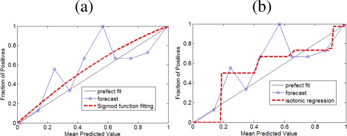
Calibration plot with fitted probabilities by (a) sigmoid fitting and (b) isotonic regression.
A quantitative measure of calibration is given by a goodness-of-fit test like the well-known Hosmer-Lemeshow test [9]. The Homer-Lemeshow C-statistic is given by:
where G denotes the number of groups (usually 10), is the sum of cases with c = 0 or c = 1, Ei is the sum of estimated probabilities, and ni denotes the number of cases in group i. This value is then compared to a chi-square distribution with G-2 degrees of freedom.
To improve the calibration of binary classification models, different calibration methods have been proposed.
Calibration Improvement
Two popular methods to improve the calibration of predictive models are the methods proposed by Platt [13] and Zadrozny and Elkan [15].
The parametric approach of Platt applies to model output rank p consists of finding the parameters A and B for a sigmoid function , such that the negative log-likelihood is minimized. However, this method may lead to poor calibration when the outputs do not fit the sigmoid function. The application of this method, referred to as sigmoid fitting, is shown in Figure 1 (a) by the dotted red line.
The non-parametric approach of Zadrozny and Elkan applies a pair-adjacent violators algorithm [2] to the previously sorted output probabilities p of the model in order to find a stepwise-constant isotonic function that best fits according to a mean-squared error criterion. However, the outputs of this calibration method tend to overfit the data if no smoothing regularization is applied. The use of this method, referred to as isotonic regression, is shown in Figure 1 (b) by the dotted red line.
Smooth non-parametric estimators are expected to alleviate overfitting and underfitting problems, and thus have received more attention recently. The methods by Wang et al. [14] and Meyer [10] find a non-decreasing mapping function t() that minimizes:
| (1) |
where m corresponds to a smoothness parameter, a and b represent the range of input predictions, and λ balances the goodness-of-fit (first component) and the smoothness (second component) of the transformation function t(). When m = 1, Equation 1 corresponds to a piece-wise linear estimator. When m = 2, Equation 1 represents a smooth monotone estimator. In theory, these models are smoother than isotonic regression and more flexible than sigmoid regression, but their inferences require much heavier computation and tedious parameter tuning. Moreover, approximation algorithms show large empirical losses, e.g. 30% using second-order cone programming [14].
Method
We intended to develop a smoother yet computationally affordable method to further improve the calibration of predictive models. We observed that isotonic regression is a non-parametric method that joins predictions into larger bins, as indicated by the flat regions in Figure 1(b). By interpolating between a few representative values, we can obtain a smoother function. However, we must ensure that such interpolation function g() is monotonically increasing to maintain the discriminative ability of the predictive model. Let P = {pi} the set of all predictions pi and C = {ci} their corresponding class labels, then the function t* () = g(f(P′), C′) is also monotonically increasing, where f() is the isotonic regression function, P′ and C′ are subsets of predictions and their corresponding class labels, repectively.
Based on these considerations, we propose a novel approximation to the optimal smooth function t*() that minimizes Equation 1 in three steps. First, we apply isotonic regression to obtain a monotone non-parametric function f() that minimizes . Second, we select s representative points from the isotonic mapping function. Finally, we construct a monotonic spline, called Piecewise Cubic Hermite Interpolating Polynomial (PCHIP) [7], that interpolates between the sampled points from the isotonic regression function to obtain a smoothed approximation to Equation 1. Note that the interpolation by PCHIP is monotonic to keep the partial ordering of the predictive model probabilities, and that it introduces the smoothness. Algorithm 1 gives the details on these steps in a compact form.
Inputs: Prediction probabilities P = p1, . . ., pn, class labels C = c1, . . ., cn
Output: Smoothed isotonic regression function h.
Obtain f* = argminf∑i (ci− f(pi))2, subject to f(pi) ≤ f(pi+1), ∀i (Isotonic Regression).
Sample s points from f*(γ), γ ∈ (0, 1), one point per flat region of f*(·). Denote samples as P′, and their corresponding class labels as C′.
Construct a Piecewise Cubic Hermite Interpolating Polynomial function t*(f*(P′), C′)) to obtain a monotone smoothing spline as the final transformation function for calibration.
Algorithm 1: Smooth Isotonic Regression
Experiments
We compare our method with sigmoid fitting and isotonic regression on the task of improving the calibration of logistic regression (LR) models learned on synthetic and real world data.
Synthetic Data
We took random samples of size n = 1000 from two Gaussian distributions with varying differences in means but fixed variances. The differences between μ1 and μ2 were set to 0.5, 1.0, 1.5 and 2.0 and the variances were set to Σ1 = 2.0, Σ2 = 1.0, respectively. We used 80% of the generated data sets to train the LR model, and 20% to test the calibration of the predictions from the LR model and the predictions after recalibration by sigmoid fitting, logistic regression, and our method.
The results of this experiment are shown in Figure 2. The blue circles in the plots are the predicted probabilities of the LR model. The red dotted lines are the recalibrated probabilities. While sigmoid fitting does not improve the calibration in all four cases, both isotonic regression and smooth isotonic regression follow the data pattern closely. They smooth isotonic regression has less oscillation and has a p-value larger than 0.05 for the H-L test indicating that the recalibrated predictions are reasonably well calibrated. We further observe that isotonic regression tends to overfit, while smooth isotonic regression provides a continuous recalibration and the highest p-values for the HL-test in most cases.
Figure 2:

Comparison of different calibration methods on synthetic data. Row one shows histograms of the original predicted probabilities by LR (blue bars for class c = 0 and red bars for class c = 1). Row two to five show calibration plots for the originall predicted probabilities of LR and the recalibrated probabilities after sigmoid fitting, isotonic regression, and smooth isotonic regression. The caption of each figure contains the discriminatory ability in terms of the area under the ROC curve (AUC) and the p-value of the HL test for the visualized probabilities.
Real World Experiment
We used eight different real world data sets. GSE2034 and GSE2990 are gene expression data sets related to breast cancer. Both data sets were preprocessed to keep only the top 15 features (see [12] for details). The HOSPITAL data consists of microbiology cultures and other variables related to hospital discharge errors of a subgroup in [5]. ADULT, BANKRUPTCY, HEIGHT_WEIGHT, MNISTALL, PIMATR were obtained from the UCI Repository [6]. MNISTALL has handwritten numbers ‘0–9’. The problem has been converted into a binary problem by treating all digits ’0’ as positive and the others as negative, yielding a very unbalanced set. For each data set, we learned an LR model on 60% random samples and tested on the remaining 40%, with the exception of the ADULT dataset, where we followed the split used in [11]. A summary of the data sets is given in Table 1. The percentage of positive cases varies from 8% to 67%.
Table 1:
Real world data sets used.
| Data | # Attr | Train size | Test size | % POS |
|---|---|---|---|---|
|
| ||||
| GSE2034 | 15 | 125 | 84 | 54 |
| GSE2990 | 15 | 54 | 36 | 67 |
| ADULT | 14 | 4,000 | 41,222 | 25 |
| BANKRUPTCY | 2 | 40 | 26 | 48 |
| HEIGHT WEIGHT | 2 | 126 | 84 | 64 |
| HOSPITAL | 22 | 2,891 | 1,927 | 8 |
| MNISTALL | 784 | 42,000 | 28,000 | 9.8 |
| PIMATR | 8 | 120 | 80 | 33 |
% POS indicates the percentage of positive cases.
Figure 3 shows histograms of the predicted values (top row) and calibration plots for the predictions of logistic regression, after sigmoid fitting, isotonic regression, and smooth isotonic regression on all eight test sets. None of the calibration methods decreases the AUC, since the monotonic transformation functions preserve the orderings. Isotonic regression sometimes shows an increase in AUC because it introduces more ties into the ranking.
Figure 3:

Comparison of different calibration methods on real world data. Row one shows histograms of the original predicted values by LR (no color discrimination for classes is used). Row two to five show calibration plots for the originally predicted probabilities of LR and the recalibrated probabilities after sigmoid fitting, isotonic regression, and smooth isotonic regression. The caption of each figure contains the discriminatory ability in terms of the area under the ROC curve (AUC) and the p-value of the HL test for the visualized probabilities.
An interesting observation gathered from the calibration plots is that they seldom display a sigmoid shape. Because the result is mostly data-driven, it discourages the use of a sigmoid function to transform predictions into probabilities (see third row). The calibration plots in the fourth row of the figure show results for isotonic regression, which are not smooth and are unrealistically sharp at the corners. The calibration plots at the bottom of the figure show the functions fitted with our proposed smooth isotonic regression, which have better performance than sigmoid fitting and less oscillation than isotonic regression. In all cases, smooth isotonic regression gives the highest p-value for the HL-test suggesting a better fit than the sigmoid approach and less overfit when compared to isotonic regression.
Conclusion
There is increasing interest in improving the calibration of predictive models, especially given their potential use for personalized medicine. While discrimination is often optimized, calibration is sometimes neglected, potentially leading to the publication of models that are not adequate for use in practice. We proposed a smooth isotonic regression method that significantly improves simple isotonic regression. The method combines the merits of parametric and non-parametric models, providing a smooth nonparametric method to improve the calibration of predictive models.
Acknowledgments
This work was funded in part by the Komen Foundation (FAS0703850), the National Library of Medicine (R01LM009520), the Austrian Genome Program (GEN-AU), project Bioinformatics Integration Network (BIN), NHLBI (U54 HL10846), and R01 HS19913-01. We thank Dr. El-Kareh for making one of the data sets available for this study.
References
- [1].Amir E, Freedman OC, Seruga B, Evans DG. Assessing women at high risk of breast cancer: a review of risk assessment models. J Natl Cancer Inst. 2010;102(10):680–691. doi: 10.1093/jnci/djq088. [DOI] [PubMed] [Google Scholar]
- [2].Ayer M, Brunk H, Ewing G, Reid W, Silverman E. An empirical distribution function for sampling with incomplete information. Annals of Mathematical Statistics. 1955;26(4):641–647. [Google Scholar]
- [3].Cohen I, Goldszmidt M. Properties and benefits of calibrated classifiers. 8th European Conference on Principles and Practice of Knowledge Discovery in Databases; 2004. pp. 125–136. [Google Scholar]
- [4].D’Agostino RB, Grundy S, Sullivan LM, Wilson P. Validation of the framingham coronary heart disease prediction scores: results of a multiple ethnic groups investigation. JAMA. 2001;286(2):180–187. doi: 10.1001/jama.286.2.180. [DOI] [PubMed] [Google Scholar]
- [5].El-Kareh R, Roy C, Brodsky G, Perencevich M, Poon EG. Incidence and predictors of microbiology results returning post-discharge and requiring follow-up. Journal of Hospital Medicine. 2010 doi: 10.1002/jhm.895. (accepted). [DOI] [PMC free article] [PubMed] [Google Scholar]
- [6].Frank A, Asuncion A. 2010. UCI machine learning repository,
- [7].Fritsch FN, Carlson RE. Monotone piecewise cubic interpolation. SIAM J Numer Anal. 1980;17(2):238–246. [Google Scholar]
- [8].Gail MH, Brinton LA, Byar DP, Corle DK, Green SB, Schairer C, Mulvihill JJ. Projecting individualized probabilities of developing breast cancer for white females who are being examined annually. J. Natl. Cancer Inst. 1989 Dec;81:1879–1886. doi: 10.1093/jnci/81.24.1879. [DOI] [PubMed] [Google Scholar]
- [9].Hosmer DW, Hosmer T, Le Cessie S, Lemeshow S. A comparison of goodness-of-fit tests for the logistic regression model. Stat Med. 1997;16(9):965–980. doi: 10.1002/(sici)1097-0258(19970515)16:9<965::aid-sim509>3.0.co;2-o. [DOI] [PubMed] [Google Scholar]
- [10].Meyer MC. Inference using shape-restricted regression splines. Annals of Applied Statistics. 2008;2(3):1013–1033. [Google Scholar]
- [11].Niculescu-Mizil A, Caruana R. Predicting good probabilities with supervised learning. International Conference on Machine Learning; 2005. pp. 625–632. [Google Scholar]
- [12].Osl M, Dreiseitl S, Kim J, Patel K, Ohno-Machado L. Effect of data combination on predictive modeling: a study using gene expression data. AMIA Annual Symposium; 2010. [PMC free article] [PubMed] [Google Scholar]
- [13].Platt JC. Probabilistic outputs for support vector machines and comparison to regularized likelihood methods. Advances in Large Margin Classifiers. 1999. pp. 61–74.
- [14].Wang X, Li F. Isotonic smoothing spline regression. J Comput Graph Stat. 2008;17(1):21–37. [Google Scholar]
- [15].Zadrozny B, Elkan C. Transforming classifier scores into accurate multiclass probability estimates. 8th ACM SIGKDD International Conference on Knowledge Discovery and Data Mining; 2002. pp. 694–699. [Google Scholar]