Visual motion integration by neurons in the middle temporal area of a New World monkey, the marmoset

Non-technical summary

The machinery of motion vision is highly conserved across New World and Old World monkeys, according to our study of the marmoset visual cortex. The marmoset is a New World primate, part of a lineage that diverged from Old World monkeys some 30–40 million years ago. A small part of the cerebral cortex, area MT, can be identified anatomically in both New and Old World primates. In the macaque, an Old World primate, this area is thought to be important in analysing the motion of complex patterns. Here we quantified the capacity of neurons in area MT of marmosets to extract motion from complex patterns. We find the responses of neurons in area MT of marmosets to be indistinguishable from those in macaques, suggesting that the functional role of this small area of the visual cortex is highly conserved over evolution.

Abstract

Abstract

The middle temporal area (MT/V5) is an anatomically distinct region of primate visual cortex that is specialized for the processing of image motion. It is generally thought that some neurons in area MT are capable of signalling the motion of complex patterns, but this has only been established in the macaque monkey. We made extracellular recordings from single units in area MT of anaesthetized marmosets, a New World monkey. We show through quantitative analyses that some neurons (35 of 185; 19%) are capable of signalling pattern motion (‘pattern cells’). Across several dimensions, the visual response of pattern cells in marmosets is indistinguishable from that of pattern cells in macaques. Other neurons respond to the motion of oriented contours in a pattern (‘component cells’) or show intermediate properties. In addition, we encountered a subset of neurons (22 of 185; 12%) insensitive to sinusoidal gratings but very responsive to plaids and other two-dimensional patterns and otherwise indistinguishable from pattern cells. We compared the response of each cell class to drifting gratings and dot fields. In pattern cells, directional selectivity was similar for gratings and dot fields; in component cells, directional selectivity was weaker for dot fields than gratings. Pattern cells were more likely to have stronger suppressive surrounds, prefer lower spatial frequencies and prefer higher speeds than component cells. We conclude that pattern motion sensitivity is a feature of some neurons in area MT of both New and Old World monkeys, suggesting that this functional property is an important stage in motion analysis and is likely to be conserved in humans.

Introduction

The middle temporal (MT) area of primate visual cortex was first functionally identified, on the basis of its topographic map of the contralateral visual field, in the New World owl monkey, where it lies exposed on the cortical surface (Allman & Kaas, 1971). Area V5 was described soon afterwards in recordings from Old World macaque monkeys, buried in the depths of the superior temporal sulcus and defined by a preponderance of neurons selective for motion direction (Dubner & Zeki, 1971). These regions are now considered homologous, but electrophysiological work on MT/V5 has since focused principally on the response properties of neurons in macaques.

The initial report of Dubner & Zeki (1971) emphasized that the directional selectivity of many neurons in area MT of macaques is distinctive in that it is preserved in the face of changes in the size or shape of a stimulus, or the orientation of the stimulus relative to its path of motion. These neurons, now commonly referred to as ‘pattern cells’, thus provide a stable neural representation of the motion of surfaces (Albright, 1984; Movshon et al. 1985; Pack & Born, 2001). This stands in contrast to the directional selectivity observed in the primary visual cortex (V1), the major input to area MT, where the great majority of neurons can only signal motion along the path perpendicular to the orientation of a contour (Hubel & Wiesel, 1968; Gattass & Gross, 1981; Felleman & Kaas, 1984; Movshon & Newsome, 1996; Priebe et al. 2003), but see Tinsley et al. (2003) and Guo et al. (2004). While quantitative analyses of motion integration in area MT of macaques do not suggest that pattern cells form a distinct class of neuron (Movshon et al. 1985; Rust et al. 2006), no study has considered the properties of their receptive fields along other dimensions. One of the aims here is to establish whether the response of pattern and component cells differ along basic dimensions of a visual stimulus.

In New World primates, which diverged from Old World monkeys some 30–40 million years ago (Glazko & Nei, 2003; Schrago & Russo, 2003), directional selectivity is also the defining functional property of neurons in area MT, but we do not know whether that selectivity depends on the orientation of contours or whether, as in macaques, some neurons are capable of signalling motion independently of spatial form. Here we apply the same quantitative methodologies that have been used to characterize the motion integration of neurons in area MT of macaques (Movshon et al. 1985; Smith et al. 2005) to neurons in the middle temporal region of a New World monkey, the marmoset. We show that in many neurons directional selectivity does not depend on the orientation of contours and that these can therefore be classed as ‘pattern’ cells. Other neurons signal the motion of particular oriented components of a stimulus and can therefore be classed as ‘component’ cells.

Methods

Ethical approval

Marmosets (Callithrix jacchus, n = 8, weighing between 350 and 430 g) were obtained from the Australian National Health and Medical Research Council (NHMRC) combined breeding facility (Churchill, Victoria, Australia). Procedures were approved by the institutional (University of Sydney) Animal Ethics Committee, and conform to the Society for Neuroscience and NHMRC policies on the use of animals in neuroscience research. The authors have read, and the experiments comply with, the policies and regulations ofThe Journal of Physiologygiven by Drummond (2009).

Experimental preparation

Each animal was initially sedated with an i.m. injection of 12 mg kg⁻¹ alfaxalone (Alfaxan; Jurox Pty Ltd, Rutherford, NSW, Australia) and 3 mg kg⁻¹ diazepam (Mayne Pharma, Mulgrave, VIC, Australia). We then gave preoperative intramuscular injections of 0.2 mg kg⁻¹ atropine (AstraZeneca, NorthRyde, NSW, Australia), to reduce lung secretions, and dexamethasone (0.3 mg kg⁻¹; Mayne Pharma), to reduce inflammation. Subsequent surgery was performed under supplemental local anaesthesia (lignocaine 2%; AstraZeneca). A femoral vein was cannulated, the trachea exposed and an endotracheal tube inserted, and the head was placed in a stereotaxic frame.

Postsurgical anaesthesia was maintained by continuous intravenous infusion of sufentanil citrate (4–12 μg kg⁻¹ h⁻¹; Sufenta Forte; Janssen Cilag, Beerse, Belgium) in physiological solution (sodium lactate; Baxter International, Toongabbie, NSW, Australia) with added dexamethasone (0.4 mg kg⁻¹ h⁻¹; Mayne Pharma) and Synthamin 17 (Amino Acids 10%; 225 mg kg⁻¹ h⁻¹; Baxter International). The ECG, EEG and arterial oxyhemoglobin saturation (via pulse oximetry) were monitored continuously. Muscular paralysis was then induced and maintained by continuous infusion of pancuronium bromide (0.3 mg kg⁻¹ h⁻¹; AstraZeneca). The animal was artificially ventilated, with a 70:30 mix of N₂O and carbogen (5% CO₂/95% O₂), so as to keep end-tidal CO₂ near 33 mmHg. EEG and ECG signals were monitored to ensure adequate depth of anaesthesia. Dominance of low frequencies (1–5 Hz) in the EEG recording and absence of EEG or ECG changes under noxious stimulus (tail pinch) were taken as the chief signs of an adequate level of anaesthesia. At any sign of the anaesthesia becoming less effective, the dose of sufentanil citrate was increased. Rectal temperature was kept near 38°C with the use of a heating blanket. Additional antibiotic and anti-inflammatory cover was given daily by intramuscular injection of 25 mg Noricillin (benzylpenicillin benzathine, Norbrook, Tullamarine, VIC, Australia) and 0.1 mg dexamethasone. The pupils were dilated with atropine sulphate and the corneas were protected with high-permeability contact lenses that remained in place for the duration of the experiment. No artificial pupils were used. At the end of the experiment, the animal was killed with intravenous administration of 500 mg kg⁻¹ sodium pentobarbitone (Lethobarb; Virbac Australia, Milperra, NSW, Australia).

Visual stimulation and recording

Supplementary lenses were used to focus the eyes at a distance of 40 or 114 cm. The power of the lenses used was determined during the course of other experiments, and is based on typical values found to maximize the spatial resolution of parvocellular cells in the dorsal lateral geniculate nucleus of the thalamus (Camp et al. 2009). Electrode penetrations were made using stereotaxic co-ordinates. A craniotomy (diameter 8–10 mm) was made over the middle temporal region, and the posterior tip of the lateral sulcus was identified. A small incision was made in the dura mater, and guide tubes containing one or two tetrodes, which were held vertically, were inserted and positioned above the cortical surface. The craniotomy was sealed with silicone elastomer. The extracellular recordings reported here were made using tetrodes (2–5 MΩ; Thomas Recordings, Giessen, Germany). The analog signals from the electrodes were amplified, bandpass filtered (0.3–10 kHz) and sampled at 48 kHz by the same computer that generated the visual stimulus. Putative spikes were displayed on a monitor, and templates for discriminating spikes were constructed by analysing multiple traces. The timing of waveforms that cohered to the template was recorded with an accuracy of 0.1 ms. Offline analysis was performed using Matlab (MathWorks, Natick, MA, USA).

In two experiments, a cathode-ray-tube monitor (ViewSonic G810; 100 Hz refresh rate, width 40 cm and height 30 cm) was viewed from 114 cm via a front-silvered mirror. In all other experiments, the same monitor was viewed directly from a distance of 45 cm. The position of the monitor was adjusted to bring the receptive field of a neuron onto the centre of the screen. Visual stimuli were generated by a G5 Power Macintosh computer using custom software (EXPO; P. Lennie, Brain & Cognitive Sciences, University of Rochester, USA); they were drawn with eight-bit resolution using commands to OpenGL. For each phosphor, we determined the relationship between the output of the video card and the photopic luminance; the inverse of this relationship was applied to the image that was sent to the video-card. All stimuli were modulated around the mean luminance (45–55 cd m⁻²) and were presented within a circular window with hard edges, outside of which the screen was held at the mean luminance.

Location of recording sites

Electrode recordings were targeted to the region 2–3 mm posterior and 2 mm lateral to the posterior tip of the lateral sulcus (Rosa & Elston, 1998). Receptive fields at the targeted location were clustered around the horizontal meridian at eccentricities near 20 deg (Rosa & Elston, 1998). In three animals, before making quantitative measurements we first made a series of electrode penetrations to map the spatial organization of multi-unit activity, and then targeted recordings towards the parafoveal representation. At the end of the experiment, the dura was reflected over the entire craniotomy, and the positioning of the electrodes relative to the posterior tip of the lateral sulcus was confirmed.

In two animals, the experiment ended prematurely and histology was not performed; in two animals, the cerebral cortex encompassing the electrode penetration was removed and fixed for 24 h in 4% paraformaldehye in 0.1 m phosphate buffer; and in four animals, the animal was perfused transcardially with 0.9% sodium chloride solution and then 4% paraformaldehye in 0.1 m phosphate buffer, and post-fixed for 24 h. The tissue was then transferred to a 30% sucrose solution in 0.1 m phosphate buffer. Coronal sections (50 μm thick) were cut on a freezing microtome, and alternate sections were stained with cresyl violet to reveal Nissl substance. We made spaced electrolytic lesions (4 μA for 6 s) along one of the tracks in each animal (the microdrive held the other electrodes at known positions relative to the electrode on which the lesions were made).

The slope of the cortical surface around area MT means that the electrode penetrations were made at an angle of ∼45 deg to the cortical surface. In each electrode penetration, isolatable neurons were recorded within 0.5 mm of encountering brain tissue (usually earlier); we recorded from neurons over an average distance of 1.3 mm, so it is likely that the majority of recordings in our sample were obtained from the superficial layers of area MT. We recovered the relevant lesions in three animals, and thus know the location of 105 neurons along six of the electrode tracks; 91 of 105 neurons were encountered across layers 2–4, and 14 were encountered in deeper layers. There was no clear functional correlate of depth within the cortex. In these animals, the myelination pattern of the cerebral cortex was revealed by a Gallyas stain performed on nearby sections (Gallyas, 1979; Bourne et al. 2007); in each case the electrode penetrations were clearly within the myelin-rich grey matter that characterizes area MT.

Stimulus sets

Stimuli were drifting sine-wave gratings or plaids, or they were fields of moving circular dots with 100% coherence and infinite lifetime, at a density of 0.3 dots s⁻¹ deg⁻¹ (each dot was 0.3 or 0.4 deg wide). Our initial set of measurements characterized the response to a drifting sinusoidal grating, as follows (gratings were of maximal contrast unless otherwise noted). For each neuron, we first established the preferred direction to a resolution of 22.5 deg. (Our reported measurements of direction tuning curves are based on responses to gratings that were obtained in conjunction with responses to plaids, as described below.) We then measured spatial frequency tuning (from 0.1 to 12.8 cycles deg⁻¹ in nine geometric steps, plus a uniform field modulated in time; the temporal frequency was usually 5 Hz), then used the optimal spatial frequency to measure temporal frequency tuning (0.55–25 Hz in eight geometric steps). We then used the preferred spatial- and temporal frequencies to measure a size tuning curve (from 0.5 to 40 deg diameter in 10 geometric steps) and then the contrast response (from 0.02 to 1.0 units of Michelson contrast in 10 geometric steps) for a grating of optimal size. In all cases, each stimulus in the set, which always included a blank screen, was presented in a pseudorandom manner for 0.5–2 s, with each measurement separated by 0.5–1 s of blank screen. The response on each trial was calculated as the mean discharge rate, in impulses per second, over the duration of the trial. For analysis of responses to these stimuli, we used the average response calculated over a median of four trials (mean five, range 2–10) of each stimulus.

We then measured the directional selectivity for drifting dot fields (from 0 to 330 deg at 30 deg intervals), and speed tuning for a dot field moving in the preferred direction (from 5 to 80 deg s⁻¹ in five geometric steps). The size of the dot field was the preferred size obtained with drifting gratings. We also measured the response to plaids and gratings (described below). In these cases, each stimulus in the set, which always included two presentations of a blank screen, was presented in a pseudorandom sequence for 320 ms, with no interstimulus interval (Smith et al. 2005). The time interval over which the response was measured was estimated as the 320 ms time segment that maximized the response variance over all stimulus conditions in the set (where the response on each trial was the average discharge rate over the appropriate 320 ms interval). This procedure is described in more detail in by Smith et al. (2005) and outlined in Fig. 1. For plaids and gratings, the average response was calculated over a median of 33 presentations of each stimulus (mean 43, range 10–168); for drifting dot fields, average response was calculated over a median of 35 presentations of each stimulus (mean 31, range 7–50).

Figure 1. Response of a neuron in middle temporal (MT) area of a marmoset to rapid serial presentation of drifting gratings and plaids.

A, rapid serial presentation of visual stimuli. The stimulus remained on the screen, drifting, for 320 ms, after which a new stimulus was chosen randomly. The set of stimuli included a blank screen and gratings and plaids drifting in each of 12 directions.B, raster plot showing the time of occurrence of action potentials, aligned to the onset of a grating drifting in the preferred direction. Each line shows one of the 43 trials of this stimulus.C, peristimulus time histogram (PSTH) of response generated from the raster plot shown inB, but over an expanded time scale. Bin width 10 ms. Example error bar shows 1 SEM.D, same asC, but for response aligned to the onset of the most effective plaid.E, procedure for estimating the optimal time window over which to analyse response. Peristimulus time histograms like those inCandDwere made for all stimuli in the set. The same latency was used for all PSTHs. From each PSTH, we obtained the average rate over a 320 ms time window following the test latency; from these estimates of average rate, we determined the variance in rate across stimuli. The position of the sliding window that maximized response variance across stimuli (here a window starting 90 ms after stimulus transition) was used for subsequent analyses. The dashed lines inCandDshow the beginning and end of this time window.

Classification of pattern and component cells

Sine-wave gratings of optimal spatial and temporal frequency and size, were presented at a contrast of 0.5. Plaids were the sum of two of these sine-wave gratings drifting at directions 120 deg apart. Both gratings and plaids were presented at each of 12 directions (from 0 to 30 deg at 30 deg intervals). To quantify the pattern directional selectivity of neurons, we computed the partial correlation of responses to a plaid with that predicted of an ideal component cell and an ideal pattern cell. The pattern cell prediction is that the response of the neuron to a plaid will be proportional to its response to a single grating moving in the average direction of the plaid; the component cell prediction as the sum of response to the two gratings that comprised the plaid. The partial correlation between the observed and ideal responses (r_component andr_pattern) were then transformed toz-scores (z_c andz_p) using Fisher'sr-to-Ztransformation. Calculating partial correlations compensates for any covariation in the predictions themselves (Movshon et al. 1985), andZ-scoring stabilizes the variance so that comparisons of the difference between partial correlation values are meaningful (Smith et al. 2005). Cells were classified as component if the correlation with the component prediction (z_c) exceeded 1.28 and the difference between the component and pattern predictions (z_c– z_p) also exceeded 1.28; the reverse criterion was applied to classify pattern cells. The criterion of 1.28 indicates significance atP = 0.90 (Smith et al. 2005).

Directional selectivity

We characterized the directional selectivity of responses to gratings and drifting dot fields; both were presented at each of 12 directions (from 0 to 330 deg at 30 deg intervals). In each case, we computed the circular variance (CV), as follows:

(1)

where θ is the motion direction of the grating or dot field, in radians, andr_kis the difference between the evoked response and the spontaneous activity, half-wave rectified. We also extracted the preferred direction, θ_pref, as the angle of the vectorRin eqn (1).

To measure the directional bandwidth, we found the best (in a least-squares sense) prediction of a wrapped Gaussian (Dakin et al. 2005), W(θ), as follows:

(2)

whereAis the gain, σ the standard deviation, μ the neuron's preferred direction, kis an integer, andballows the entire curve to be offset and was constrained to be greater than or equal to zero. We characterize the bandwidth of these tuning curves as the standard deviation, σ. Parameters providing the best-fitting predictions of this model, and all other models described here, were found using thelsqcurvefitfunction in Matlab, which minimized the square error between the model predictions and the evoked response (the difference between the response rate and the spontaneous activity, half-wave rectified). To characterize the quality of the predictions provided by the model, we computed the percentage of variance across stimuli for which the model accounted (Carandini et al. 1997).

Speed response

To describe the speed-response curves, we found the best predictions of a difference of two exponentials (not shown; Derrington & Lennie, 1984), as follows:

(3)

where ω is the speed of the stimulus, A₁ andA₂ the excitatory and inhibitory gains, and τ₁ and τ₂ the excitatory and inhibitory time constants.

Contrast response

To describe the contrast response, we found the best prediction of the Naka–Rushton function (Sclar et al. 1990), as follows:

(4)

wherecis the contrast, R_max the maximal attainable response, c₅₀ a semi-saturation constant (the contrast at which response reaches half its maximal value), andMis the spontaneous rate of discharge. The semi-saturation constant, c₅₀, gives a measure of the contrast required for a response from the neuron. To measure the sensitivity of neurons to changes in contrast, the slope aroundc₅₀, we usednR_max/4c₅₀; this is obtained by differentiating eqn (4) with respect toc, and then substitutingc₅₀, thereby providing the slope atc₅₀.

Statistical analysis

A Wilcoxon rank sum test was used to determine, across functional types of neurons, the significance of differences in the directional CV and bandwidth, spatial and temporal frequency tuning, speed tuning and contrast response. Student's pairedttest was used to determine the significance of changes in directional selectivity (CV and bandwidth) for a single neuron stimulated with gratings or dot fields. We performed a bootstrap analysis to obtain confidence limits for each data point in our analyses of the temporal dynamics of response. We drew a new sample of the same size (randomly, with replacement) from the set of measurements available, and calculated the mean of that resample. We repeated the procedure 1000 times, sorted the resultant estimates of mean, and found the 25 and 975 elements. These provide 95% confidence intervals on each of the mean values shown.

Results

The response properties described here are drawn from a data set of 318 single units recorded at 177 sites within the middle temporal region of visual cortex of eight marmosets. For 247 of these neurons, we measured direction tuning curves for gratings and plaids, and thus characterized the manner in which the neuron integrates motion signals. For 42 of these neurons, the average response during presentation of a grating or a plaid did not exceed 10 impulses s⁻¹; these were excluded from most of the following analyses. Twenty of the remaining 205 neurons (10%) were classed as orientation selective because the response to the preferred direction was no more than twice that to the anti-preferred. In what follows, we generally limit our observations to the remaining 185 direction-selective neurons. We first show that the direction tuning of a significant proportion of neurons was similar for plaids and gratings, and the receptive fields of these neurons were therefore ‘pattern’ selective; the remaining neurons were selective for the components of the plaids, or had intermediate response patterns. We go on to characterize the tuning of these functional classes along additional stimulus dimensions; in each case, a neuron was excluded from the relevant analyses if the mean evoked rate did not exceed the spontaneous rate by 10 impulses s⁻¹.

Pattern, component and unclassified cells

Figure 2A–D shows the direction tuning curves of four neurons, measured with a grating (filled circles) or a plaid (open circles). In each case, the response to a grating is shown as a function of the motion direction of that grating. The response to a plaid is shown as a function of the average direction of its two component gratings, which corresponds to the direction of pattern motion (the motion directions of the component gratings were separated by 120 deg). The neurons in Fig. 2A–C show similar directional selectivity for gratings, the curves have a clearly defined single peak, which has been arbitrarily set to 0 deg here. The responses of these neurons to the plaid are markedly different; the tuning curve for the neuron in Fig. 2A shows two peaks, separated by 120 deg; for the neuron in Fig. 2B, the plaid tuning curve is single peaked, but is substantially broader than the curve for gratings; for the neuron in Fig. 2C, the tuning curves for plaids and gratings are very similar.

Figure 2. Motion integration of four neurons from area MT of a marmoset.

Each panel shows mean rate over a 320 ms period, for drifting gratings (contrast 0.5; filled circles) and plaids formed by linear superposition of two gratings with directions 120 deg apart (open circles). In each case, responses have been aligned such that the preferred direction for a grating is 0 deg; the direction of the plaid is the average of its two components, aligned to the preferred direction for a grating. The dotted curve shows the predicted response of an ideal component cell to the plaid (see Methods); the predicted response of an ideal pattern cell is that it will respond in the same way to the grating and the plaid. The classification of neurons inA–Cis based on the metrics shown in Fig. 3A.A, component cell. Same cell as Fig. 1.B, unclassified cell.C, pattern cell.D, one of the neurons in our sample with robust and unimodal responses to plaids but weak response to gratings. The grating response is insufficient to classify the motion selectivity of the neuron. Stimulus parameters for the neuron inAare as follows: spatial frequency 0.8 cycles deg⁻¹; temporal frequency 11.1 Hz; size 11.0 deg. For the neuron inB, these parameters were 0.25 cycles deg⁻¹, 16.7 Hz and 16.9 deg; for the neuron inC, 0.2 cycles deg⁻¹, 10.0 Hz and 20.0 deg; and for the neuron inD, 0.4 cycles deg⁻¹, 10.0 Hz and 7.0 deg. Error bars inA–Dshow 1 SEM.

To categorize neurons quantitatively, we compared the response to a plaid with that predicted for ideal component and pattern cells (Movshon et al. 1985; see Methods). The response of an ideal pattern cell should not depend on the orientation content of the stimulus, and so the tuning curve for a grating serves as the predicted tuning curve for a plaid. An ideal component cell should respond independently to the separate gratings that comprise the plaid and the direction tuning curve for plaids will therefore be bi-lobed (the sum of the responses to the individual gratings). The dotted curves in Fig. 2A–C show in each case the response to the plaid that would be expected were the neuron an idealized component cell. For each neuron, we calculated the partial correlation between the response to plaids and the predicted response for pattern cells (providing the metricz_p) and component cells (z_c).

Figure 3 compares the two partial correlations for the population of neurons. The example neurons whose tuning curves are shown in Fig. 2 are indicated by the triangles. Neurons were classified as component cells if the correlation with the component prediction (z_c) exceeded 1.28 and the difference between the component and pattern predictions (z_c– z_p) also exceeded 1.28; the reverse criterion was applied to classify pattern cells. The criterion of 1.28 indicates significance atP = 0.90 (Smith et al. 2005); the dashed lines in Fig. 3A separate the plot into regions of component, pattern and unclassified cells. Figure 3B shows a histogram of the difference between the partial correlations (z_c– z_p), equivalent to collapsing the plot in Fig. 3A along the diagonal. There is no sign of discrete classes of cells.

Figure 3. Quantification of motion integration across a population of neurons in area MT of a marmoset.

For each neuron, we compared response to plaids with that predicted for ideal component and pattern cells by computing the partial correlation with each prediction.A, a scatter plot of the partial correlation between measured response and that of an ideal component cell (z_c) or ideal pattern cell (z_p). The dashed lines separate regions of pattern (open symbols), unclassified (grey symbols) and component cells (filled symbols; see Methods). Open symbols not in the pattern region of the plot mark neurons, such as that in Fig. 2D, that have very weak responses to gratings and in which the pattern cell prediction is therefore compromised. Triangles mark the neurons shown in Fig. 2. Neurons in whichz_c is less than −1.28 are plotted on the abscissa.B, the distribution of the difference inz_c andz_p. Open bars show pattern cells, grey bars show unclassified cells and filled bars the component cells. Neurons with responses like those in Fig. 2D are not included in the distribution.

By these criteria, 35 of 185 neurons (19%; open symbols) were classified as pattern cells, which is similar to the proportions reported for the Old World macaque monkey (Movshon et al. 1985; Smith et al. 2005). Sixty-seven neurons (36%; filled symbols) were classified as component cells. In the following, we have included in our population of pattern cells 22 additional neurons that were weakly responsive or unresponsive to a grating but very responsive to a plaid (they are excluded from the histogram in Fig. 3B). The plaid tuning curve of these neurons was always single peaked, and the response of one neuron is shown in Fig. 2D. We saw no neurons that responded robustly to gratings but were unresponsive to plaids. The absence of a robust grating tuning curve compromises the classification described above, because the predicted responses of ideal pattern and component cells are generated from responses to a grating. To make sure that our estimate of a neuron's ‘pattern-ness’ or ‘component-ness’ was not corrupted by the absence of a robust response to gratings, we inspected the grating and plaid tuning curves of all neurons. In the following analyses, the population of pattern cells will include those that we identified manually; the open circles in Fig. 3A that do not lie within the ‘pattern’ region are these neurons. When we include these neurons, the proportion of pattern cells in the population of MT neurons is 31% (57 of 185).

The spontaneous and evoked discharge rate was similar for all three cell groups; the mean spontaneous rate of component cells was 4.9 impulses s⁻¹ (median 4.4; SD 5.0), of pattern cells 6.0 impulses s⁻¹ (median 3.4; SD 7.0) and of unclassified cells 5.5 impulses s⁻¹ (median 3.4; SD 5.6). The average evoked rate (in response to their optimal plaid or grating) over the entire 320 ms analysis epoch was for component cells 36.6 impulses s⁻¹ (median 29.8; SD 22.2), for pattern cells 44.5 impulses s⁻¹ (median 32.8; SD 32.9) and for unclassified cells 44.5 impulses s⁻¹ (median 31.2; SD 25.1).

Temporal dynamics of motion integration

In area MT of both anaesthetized and awake macaque, there is substantial evidence that response to a plaid evolves over the ∼150 ms following the onset of a stimulus (Pack et al. 2001; Smith et al. 2005). The responses described in the previous section were obtained using stimulus sets identical to those used by Smith et al. (2005), and we could therefore investigate whether this temporal evolution was also evident in neurons in area MT of marmosets.

We compiled peristimulus time histograms (PSTHs) of the response to each stimulus at a resolution of 10 ms, aligning responses to the onset of that stimulus. For each 10 ms bin in the PSTH, we calculated the partial correlations as above (z_p andz_c), providing an instantaneous measure of pattern- or component-like behaviour. For comparison with previous work, we also calculated partial correlations for the cumulative response from stimulus onset to the time bin under study. We include neurons whose response in any time bin exceeded 10 impulses s⁻¹ above the spontaneous rate for at least one grating and one plaid. This criterion accepts neurons with very transient responses, and thus adds neurons to our data set, most of which were component cells. A total of 224 cells met the criteria; from the cumulative response over the 320 ms stimulus period we identified 90 component cells, 50 pattern cells and 84 unclassified.

We first examined the pattern and component classification as a function of the cumulative response in each time bin. It is easiest to see this as the trajectory of a neuron within the plot ofz_p againstz_c. Figure 4A shows the evolution of the averagez_p andz_c values for the three groups of neurons. The first spikes from a neuron are not related to the stimulus, and so for all groups the trajectory starts near the origin of the plot. The initial response of the neuron is often not reliable enough to classify it; it is only when sufficient spikes are accumulated that the estimate is reliable and the trajectory moves away from the origin in the direction of the ultimate classification. Component cells were on average reliably classifiable within 90 ms of the onset of stimulus. Pattern cells were not reliably classifiable until 160 ms. The difference is made clearer in Fig. 4B, which shows the evolution of the difference inz_p andz_c for pattern and component cells. For pattern cells, we showz_p–z_c to indicate pattern selectivity; for component cells, we showz_c–z_p to indicate component selectivity. The dotted horizontal line shows the usual significance boundary (1.28). Figure 4B makes clear that component-like behaviour is rapidly and reliably classified, but that pattern-like behaviour takes longer to emerge. Figure 4C shows that these distinct temporal patterns are also present ifz_p andz_c are calculated from the response in each time bin, not the cumulative response.

Figure 4. Temporal evolution of plaid response in pattern cells and component cells.

A, mean trajectory ofz_c andz_p for pattern cells (n = 50; open circles), unclassified cells (n = 84; grey circles) and component cells (n = 90; filled symbols). For each neuron, we calculatedz_c andz_p for the cumulative response, in bins of 10 ms, so the bins marked ‘100’ show the averagez_c andz_p values obtained for responses up to 100 ms following onset of the stimulus. Neurons were classified on the basis of response over the entire 320 ms analysis window. The numbers along each line show the time of the relevant datum in milliseconds, relative to onset of the stimulus. The dashed lines separate regions of pattern, unclassified and component cells.B, evolution of pattern selectivity in pattern cells (z_p–z_c) and component selectivity in component cells (z_c–z_p). The dashed horizontal line replots the relevant significance boundary fromA. In this plot, partial correlations were calculated from the cumulative response, as was done inA.C, same asB, but with partial correlations calculated for each 10 ms time bin independently. Error bars inBandCshow 95% confidence intervals for the mean obtained by bootstrapping.

Among all component cells, the trajectories of individual neurons closely followed that of the average shown in Fig. 4AandB, and moved smoothly from the unclassified into the component region of the plot (one component cell meandered through the pattern region). This was also the case for 28 of 50 pattern cells (56%). In 22 (44%) pattern cells, the trajectory was different; in these cells, the trajectory moved through the component region of the plot before reaching the pattern region. This is similar to observations in macaques (Smith et al. 2005; see also Pack & Born, 2001) and is consistent with the idea that the computation of pattern motion takes time. The response of unclassified cells was variable; two of 84 (2%) could be described as a pattern cell and 34 (40%) could be described as a component cell at some point during the temporal evolution of their response.

Temporal dynamics of direction tuning

The spatial tuning of neurons in V1 of macaques and cats is often broader in the initial response to a stimulus, and narrows over time (Ringach et al. 1997; Bredfeldt & Ringach, 2002; Mazer et al. 2002). The temporal dependence of pattern cell classification shown in the previous section may suggest similar changes in the receptive field properties of neurons in area MT. Indeed, if tuning width or response amplitude evolved more slowly in pattern cells than in component cells, it may have helped to generate the lag in pattern cell classification.

We first considered the possibility that the visual response latency of pattern cells is substantially greater than that of other cells. This was not the case. The visual response latency was estimated, to 10 ms resolution, by finding the start of a 320 ms time window that maximized response variance across all stimuli (both gratings and plaids; see Methods and Fig. 1; Smith et al. 2005). For pattern cells, response latency was on average 85.4 ms (median 80, SD 17.6, n = 50), for component cells 83.4 ms (median 80, SD 17.2, n = 90) and for unclassified cells 83.5 ms (median 80, SD 18.1, n = 84). At this temporal resolution, no cell class responded more rapidly than another; higher temporal resolution, requiring more trials than we generally obtained, might reveal more subtle differences (Smith et al. 2005). Note that this is a conservative measure of response latency because it takes into account response to all stimuli and not only the most effective ones.

We then asked whether, for gratings, the response amplitude or tuning developed more slowly in pattern cells than in component cells. Figure 5A shows for each cell class the average direction tuning curve at 100 ms after a stimulus transition, and 300 ms after. In each case, the tuning curve of each cell was aligned to the preferred stimulus direction; the amplitude of each neuron was normalized to that in response to a preferred grating, averaged across the entire 320 ms window. On average, the amplitude of the tuning curve reduces slightly over time, particularly for component cells. Early on in the response, component cells also show a small response to the anti-preferred direction. In neither pattern nor component cells is there a clear change in the bandwidth of the tuning curve over time.

Figure 5. Temporal evolution of response gain and directional selectivity in pattern cells and component cells.

For each neuron, we measured responses to 12 directions of a drifting grating of contrast 0.5.A, average direction tuning curves for pattern and component cells for response obtained in a single 10 ms bin, either 100 ms after stimulus transition (upper panels) or 300 ms after (lower panels). In each case, stimulus direction was aligned to that preferred in the time bin under study. Response was normalized to that for the preferred direction, averaged over the entire 320 ms analysis window.B, average PSTH in response to a grating moving in the preferred direction, for pattern cells (open circles) and component cells (filled circles). For each neuron, spontaneous activity was subtracted and response normalized to the average over the entire 320 ms analysis window. Bin width 10 ms.C, circular variance as a function of time. Measurements were made independently in each 10 ms bin. Conventions are as inB. Error bars inA–Cshow 95% confidence intervals on the mean obtained by bootstrapping.

Figure 5B shows the average PSTH of pattern and component cells to presentation of a drifting grating moving in the preferred direction. For each cell, the spontaneous activity was subtracted and response then normalized to the average response over the entire 320 ms stimulus duration. In each cell class, the response starts to rise rapidly at 70 ms after a stimulus transition, reaches a peak around 100 ms after stimulus transition and then diminishes to an asymptotic level at 150 ms. There is no evidence for a substantially longer time to peak in pattern cells than in component cells.

Figure 5A suggests that in both cell classes the bandwidth of the direction tuning curve is stable over time; to establish this quantitatively, we analysed the direction tuning curves in every 10 ms bin following stimulus transition. The shape of a direction tuning curve is well captured by its circular variance (CV; see Methods; Mardia, 1972); a value of zero indicates that a neuron responds to only one direction, and a value of one indicates that a neuron responds equally well to all directions. Figure 5C shows that once they are responding robustly, the tuning width of both pattern and component cells, as measured by the circular variance, is stable across the analysis window.

The general stability of directional selectivity in pattern cells in response to gratings stands in contrast to the slow evolution of pattern motion integration. Eighty to ninety milliseconds after a stimulus transition, there is little difference in the response amplitude or circular variance of pattern and component cells (Fig. 5), but motion integration in pattern cells is not yet reliably classifiable (Fig. 4BandC). The slower emergence of pattern-like behaviour, therefore, does not simply reflect differences between pattern and component cells in the sensitivity or tuning for gratings (and thus the accuracy of the predictions), but rather the fact that it can take time for pattern-like behaviour to emerge.

Stimulus dependence of direction tuning

Directional selectivity is the physiological hallmark of neurons in area MT (Dubner & Zeki, 1971; Van Essen et al. 1981; Albright, 1984; Movshon et al. 1985), but we know much less about how directional selectivity depends on the stimulus used to measure it. Figure 6 shows the direction tuning curves for drifting gratings and dot fields in the same neurons shown in Fig. 2. Clear trends emerged when we compared directional selectivity for dots and gratings in individual cells. Component cells, such as that in Fig. 6A, show narrow tuning curves for gratings and broader tuning curves for dot fields. This is not the case for pattern cells (Fig. 6C), where the two tuning curves have similar shape. Unclassifiable cells (Fig. 6B) show intermediate behaviour. The pattern cell in Fig. 6D, which responds to plaids but not gratings, also responds robustly to dot fields. This was the case for all pattern cells that lacked robust responses to gratings; the responses of these cells to plaids and dot fields were indistinguishable from those of other pattern cells. In this section, we compare responses to fields of drifting dots and gratings, so neurons were included only if they responded more than 10 impulses s⁻¹ above the spontaneous rate to both.

Figure 6. Response of four neurons to drifting gratings and dot fields.

Same neurons as Fig. 2. Each panel shows the mean rate of one neuron during 320 ms presentation of a drifting grating (filled circles) at the preferred temporal frequency, and a dot field (open circles) drifting at the preferred speed. The grating responses are replotted from Fig. 2. Dot size was 0.4 deg, and all dots drifted in the same direction with infinite lifetime. For the neuron inA, the dot field was of size 16.9 deg, and dots drifted at a speed of 10.0 deg s⁻¹. For the neuron inB, these parameters were 16.9 deg and 40.0 deg s⁻¹; for the neuron inC, 11.0 deg and 30.0 deg s⁻¹; and for the neuron inD, 7.0 deg and 10.0 deg s⁻¹. Error bars inA–Dshow 1 SEM.

To characterize the direction tuning curves across the population, we used two widely used metrics: the circular variance (CV) described above, which reflects global directional selectivity because it uses the responses to all directions, and the bandwidth of a Gaussian fit to the response, which provides the sharpness of tuning around the peak. These two metrics therefore give complementary descriptions of the direction tuning curves of our population of neurons. For example, CV can be relatively high in neurons that respond best to a limited range of directions around their preferred direction, but nevertheless respond above baseline to most directions. In practice, there was a high correlation between the two metrics, particularly for tuning curves measured with drifting dot fields. For dot fields, the correlation coefficient (r) was 0.53, 0.57 and 0.84 for pattern, unclassified and component cells, respectively; for gratings, these values were 0.75, 0.43 and 0.43. Confidence intervals overlapped for all possible comparisons. For completeness, we provide both metrics; for a full discussion of their relationship, the reader is directed to Ringach et al. (2002).

Figure 7A shows for drifting gratings the distributions of CV for component cells, unclassified cells and pattern cells. For gratings, the CV of component and pattern cells was similar (see also Fig. 5C). Figure 7B shows the equivalent measurement for responses to drifting dot fields. Reflecting the broader tuning curves in Fig. 6A, component cells have a larger CV than pattern cells (P< 0.01) for dot fields. We also compared the two tuning curves in individual neurons. In component cells, CV was greater for dot fields than gratings (P< 0.05). In contrast, pattern cells had a greater CV for gratings than dot fields (P< 0.05).

Figure 7. Directional selectivity of neurons in area MT derived from measures of circular variance (CV).

Each panel shows the distribution of CV (see Methods) for mean rate. Values of one indicate neurons with equal response to all directions; values of zero indicate neurons with response to only one direction. Tuning curves were made from responses to equally spaced 12 directions, as shown in Fig. 6. Arrows show the distribution mean.A, CV of response to drifting gratings of preferred temporal frequency. Mean CV of component cells is 0.25 (median 0.18, SD 0.19, n = 36); of unclassified cells 0.31 (median 0.27, SD 0.22, n = 32); and of pattern cells 0.27 (median 0.21, SD 0.18, n = 32).B, CV of response to drifting dot fields of preferred speed. Same populations of neurons as inA. Mean CV of component cells is 0.30 (median 0.26, SD 0.17); of unclassified cells is 0.30 (median 0.23, SD 0.17); and of pattern cells is 0.20 (median 0.17, SD 0.11).

The bandwidth of each tuning curve was estimated by finding the best predictions of a circular Gaussian (see Methods). Figure 8A shows the distributions of bandwidth (one standard deviation of the Gaussian) for a drifting grating, and Fig. 8B shows the same measure for a drifting dot field. Seven pattern cells and four unclassified cells were excluded from these histograms because the model accounted for less than 60% of the response variance for either gratings or dot fields (Carandini et al. 1997). For gratings, component cells have narrower bandwidths than pattern cells (P< 0.0001), but for dot fields component cells have broader bandwidths (P< 0.05). In individual component cells, bandwidth was narrower for gratings than for dot fields (P< 0.0001); in pattern cells, bandwidth was not significantly different for the two types of stimuli (P = 0.63). In summary, for pattern cells directional selectivity is largely invariant with stimulus, but for component cells it is not.

Figure 8. Directional selectivity of neurons in area MT derived from measures of bandwidth.

The best prediction of a circular Gaussian was found for the mean rate of each neuron (see Methods). Each panel shows the distribution of the standard deviation of this Gaussian. Conventions as in Fig. 7.A, bandwidth of response to drifting gratings of preferred temporal frequency. Mean bandwidth of component cells is 22.0 deg (median 18.8, SD 13.5, n = 36); of unclassified cells is 26.4 deg (median 27.8, SD 13.8, n = 28); and of pattern cells is 34.1 deg (median 34.7, SD 11.6, n = 25).B, bandwidth of response to drifting dot fields of preferred speed. Same population of neurons as inA. Mean bandwidth of component cells is 44.2 deg (median 45.6, SD 17.1); of unclassified cells is 42.0 deg (median 39.5, SD 15.36); and of pattern cells is 34.9 deg (median 35.7, SD 8.9).

Spatial and temporal tuning of pattern and component cells

For each neuron, we measured the tuning for spatial frequency, temporal frequency and size of a patch of grating drifting in the optimal direction. Examples of these measurements are shown for one pattern cell and one component cell in Fig. 9A–C. In each case, we fitted descriptive functions to the underlying data; we used a difference of Gaussians (Enroth-Cugell & Robson, 1966) to describe the spatial frequency tuning curve, a difference of exponentials (Derrington & Lennie, 1984) for temporal frequency, and a two-dimensional difference of Gaussians (Cavanaugh et al. 2002) for the size tuning curve.

Figure 9. Tuning properties of neurons in area MT obtained using drifting gratings.

A–C, mean rate of two example neurons in response to drifting gratings, as a function of the spatial frequency (A), temporal frequency (B) or size (C) of that grating. One neuron is a pattern cell (grey open symbols and dashed lines); the other is a component cell (filled symbols and continuous lines). The lines show the best-fitting predictions of descriptive functions fitted to the data in each panel.D, distribution of characteristic spatial frequency for component cells (top panel), unclassified cells (middle panel) and pattern cells (bottom panel). This parameter indicates the spatial frequency resolution of each neuron. Arrows show the means of the distributions. Mean frequency is 1.3 cycles deg⁻¹ (median 1.11, SD 0.85, n = 55) for component cells, 0.91 cycles deg⁻¹ (median 0.68, SD 0.80, n = 46) for unclassified cells and 0.82 cycles deg⁻¹ (median 0.66, SD 0.6, n = 48) for pattern cells.E, distribution of preferred temporal frequency. Conventions as inD. Mean frequency is 10.2 Hz (median 9.4, SD 4.8, n = 47) for component cells, 10.8 Hz (median 10.6, SD 5.3, n = 40) for unclassified cells and 11.62 Hz (median 10.2, SD 6.2, n = 43) for pattern cells.F, distribution of preferred grating size. Conventions as inDandE. Mean size was 14.8 deg (median 15.1, SD 8.2, n = 27) for component cells, 11.8 deg (median 10.2, SD 6.3, n = 30) for unclassified cells and 14.1 deg (median 12.5, SD 8.4, n = 24) for pattern cells.

Figure 9D shows the distributions of characteristic spatial frequency for the cells in our sample. The characteristic frequency (f_c) describes the spatial frequency resolution of each neuron (f_c = 1/πr_c, wherer_c is the radius of the ‘centre’ mechanism in the difference-of-Gaussian model). Figure 9D makes clear that, overall, component cells can resolve higher spatial frequencies than pattern cells (P< 0.001). The preferred spatial frequency of component cells is also higher than that of pattern cells (data not shown); the preferred spatial frequency of MT neurons here was on average 0.24 cycles deg⁻¹ (geometric mean), similar to that reported previously for marmoset area MT (Lui et al. 2007). All cells showed strong roll-off at low spatial frequencies, and were generally unresponsive to temporal modulation of a uniform field.

Our ability to estimate temporal resolution accurately was limited by the fact that many neurons were still highly responsive at the highest drift rate we could generate, 25 Hz. Figure 9E shows instead the distribution of preferred temporal frequencies for each cell class. The preferred temporal frequency across the population of MT cells was 9.25 Hz (geometric mean). This is higher than has been reported previously (Lui et al. 2007). Figure 9E indicates substantial overlap in the distributions of preferred temporal frequency in pattern cells and component cells; their means do not differ significantly (P = 0.20).

The optimal diameter of a patch of drifting grating was on average 13.6 deg. Figure 9F shows that the optimal size was similar for pattern and component cells (P = 0.80). All three cell groups were encountered at comparable parafoveal and peripheral eccentricities; the mean eccentricities for component, unclassified and pattern cells were, respectively, 23.9 (SD 13.0), 23.6 (SD 10.4) and 22.1 deg (SD 8.5).

Speed tuning

The analysis of visual motion requires estimation of direction and speed (Newsome & Pare, 1988; Britten et al. 1992). Figure 9 shows that component cells are sensitive to higher spatial frequencies than pattern cells, and prefer similar temporal frequencies. The prediction is therefore that pattern cells will be sensitive to higher speeds (which are the ratio of temporal to spatial frequency).

To measure speed tuning, we obtained responses to a drifting dot field of varying speed in 114 neurons (the diameter of each dot was 0.4 deg; the diameter of the field was that estimated from the size tuning curves in the previous section). To characterize the tuning, we fitted responses to the prediction of a difference-of-exponentials model, and from this extracted the preferred speed. The tuning curves could be very broad, and in many cells we could not estimate the maximal or minimal resolvable speed. Figure 10 shows the distribution of preferred speed for component, unclassified and pattern cells. Twenty-two (19%) neurons preferred speeds above the maximal speed tested (80 deg s⁻¹), and eight (7%) preferred speeds below the minimal speed tested (5 deg s⁻¹); the grey bars in Fig. 10 show these. Among neurons with measureable preferred speeds, pattern cells prefer higher speeds than component cells (P< 0.01).

Figure 10. Distributions of preferred speed for neurons in area MT obtained using drifting dot fields.

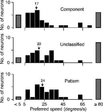
Distribution of preferred speed for component cells (top panel), unclassified cells (middle panel) and pattern cells (bottom panel). Arrows show the mean of the distributions for neurons with preferred speed between 5 and 80 deg s⁻¹. Mean speed is 17.4 deg s⁻¹ (median 12.8, SD 18.1, n = 41) for component cells, 19.8 deg s⁻¹ (median 16.6, SD 13.8, n = 34) for unclassified cells and 24.2 deg s⁻¹ (median 22.2, SD 14.4, n = 40) for pattern cells.

Motion opponency and gain controls

Most models of motion integration suggest that its emergence requires a motion-opponent stage and additional suppressive mechanisms (Wilson et al. 1992; Simoncelli & Heeger, 1998; Rust et al. 2006). A direction index (DI) was used to quantify motion opponency in each neuron, as follows:

(5)

wherer_pref is the response (after subtracting the spontaneous rate) to the stimulus moving in the preferred direction, andr_anti-pref is the response to the opposite direction. Most cells, irrespective of classification, had a DI greater than one for both gratings and dot fields, indicating that over all cell classes the discharge falls below the spontaneous rate during presentation of anti-preferred motion (Snowden et al. 1991). The mean DIs for component cells were 0.94 (median 1.01, SD 0.31) and 1.04 (median 1.01, SD 0.30, n = 43) for gratings and dot fields, respectively. For pattern cells, these were a mean of 1.31 (median 1.02, SD 1.83) and 1.02 (median 1.01, SD 0.07, n = 42), and for unclassified cells they were 1.52 (median 1.02, SD 3.64) and 0.98 (median 1.03, SD 0.22, n = 41). These results show that pattern and component cells are not distinguished by the presence or absence of motion opponency, though we note that this measure cannot quantify opponency that is concealed by spike threshold.

A general indicator of the presence of contrast gain controls is the shape of the contrast response function. We therefore measured the contrast response of 108 neurons to a drifting grating of optimal spatial and temporal frequency and optimal size. To characterize the responses, we found the best-fitting predictions of a Naka–Rushton function (eqn (4); see Methods). From these fits, we extracted two measures that capture the contrast sensitivity: the semi-saturation constant, c₅₀, and the slope of the curve atc₅₀ (nR_max/4c₅₀). Thec₅₀ characterizes the range of contrasts over which the neuron responds differentially; stronger gain controls will lead to saturation of response at lower contrast levels, and therefore lower values ofc₅₀. The slope captures the rate of change of response (in impulses per second per unit contrast) over the dynamic range of the neuron under study. In this analysis, we allowed neurons that did not respond above 10 impulses s⁻¹ but were nevertheless captured by the Naka–Rushton function (6 neurons in which the response was too variable were excluded).

Figure 11A shows the distribution ofc₅₀ values for component, unclassified and pattern cells. For neurons where the response at high contrast saturates little or not at all, c₅₀ is high and poorly constrained; the grey bars show those neurons withc₅₀ above 0.5. There was no difference in thec₅₀ values between component cells and pattern cells (P = 0.70). Figure 11B shows the distributions of our estimate of contrast sensitivity (slope) for component, unclassified and pattern cells. The distributions overlap substantially, and there is no difference in the average slope (P = 0.48).

Figure 11. Distributions of contrast sensitivity of neurons in area MT obtained using drifting gratings.

AandB, distributions for component cells (top panel), unclassified cells (middle panel) and pattern cells (bottom panel).A, distributions of the semi-saturation constant of the Naka–Rushton function, c₅₀. Arrows show the mean for neurons with ac₅₀ below 0.5. Meanc₅₀ is 0.16 (median 0.15, SD 0.10, n = 36) for component cells, 0.11 (median 0.10, SD 0.08, n = 32) for unclassified cells and 0.15 (median 0.11, SD 0.11, n = 34) for pattern cells.B, distributions of the slope atc₅₀. Conventions as inA. Mean slope is 265 impulses s⁻¹ (unit contrast)⁻¹ (median 119, SD 396, n = 36) for component cells, 330 impulses s⁻¹ (unit contrast)⁻¹ (median 175, SD 358, n = 32) for unclassified cells and 275 impulses s⁻¹ (unit contrast)⁻¹ (median 113, SD 365, n = 34) for pattern cells.

Several models of motion integration require tuned suppression (Rust et al. 2006; Tsui et al. 2010); one source of this may be suppressive surrounds, which in V1 and MT cells are often tuned for the direction of motion of a moving stimulus (Allman et al. 1985). We therefore measured the strength of surround suppression in each of the three classes of MT neurons. In most marmoset MT neurons, the response diminished as a grating patch was increased from its optimal size to the largest we could generate (diameter 20–40 deg; Fig. 9C). We characterized this suppression as the percentage reduction in response at the largest size, such that 0% indicates no suppression and 100% complete suppression. Pattern cells showed significantly more suppression than component cells (P< 0.05). On average, the suppression index for component cells was 40% (SD 30%, n = 26), for pattern cells 60% (SD 32%, n = 24) and for unclassified cells 54% (SD 33%, n = 30).

Discussion

We have identified neurons in the middle temporal area of the marmoset where direction tuning is preserved in the face of substantial changes in the orientation content of moving patterns. The motion integration performed by these neurons is indistinguishable from that performed by ‘pattern cells’ identified in area MT of macaques using the same methods. Our observations therefore show that pattern motion sensitivity is a property of neurons in area MT that is conserved across New and Old World primate lineages, consistent with the idea that this an important stage in motion analysis. As in the Old World primates, we also observed cells that responded independently to the separate spatiotemporal elements of complex visual stimuli, resembling ‘component cells’ described in macaques, as well as cells with motion integration properties intermediate to the pattern and component classes. There were no clear qualitative differences in the other functional properties of neurons in each cell class, but there were quantitative differences. In the following discussion, we briefly compare the properties of pattern cells and component cells in macaques and marmosets. We then consider how present models of motion integration address the quantitative differences in their receptive field properties.

Pattern direction sensitivity in New and Old World primates

Neurons are pattern motion sensitive when their directional tuning is largely invariant to changes in the spatial structure of a moving surface. We established that invariance here by quantitatively comparing the response to a drifting grating, which has a single orientation, with the response to a drifting plaid, which has two orientations, a technique that has been widely applied to neurons in area MT of the macaque. On the basis of the partial correlation metrics, the proportion of pattern (19%) and component cells (36%) in our sample from the middle temporal region of marmosets is similar to that reported in macaques (22–28% pattern cells and 23–52% component cells; Movshon et al. 1985; Priebe et al. 2003; Smith et al. 2005; Rust et al. 2006). Furthermore, in our sample, as in macaques, the distribution of the difference in partial correlations (z_c– z_p) is unimodal and biased towards the component classification (Rust et al. 2006), the classification of pattern cells took longer to arise than that of component cells, and in each cell class the time course and trajectory of classification were very similar to those observed in macaques (Smith et al. 2005).

This is in accord with previous work showing that the following functional properties of area MT in New and Old World primates are similar: the preponderance of directionally selective neurons, the large size of receptive fields relative to those in area V1 (Gattass & Gross, 1981; Felleman & Kaas, 1984), the presence of neurons that are selective for the speed of a drifting grating rather than its spatial and temporal frequency (Perrone & Thiele, 2001; Lui et al. 2007), the prevalence of strong suppressive surrounds (Allman et al. 1985; Tanaka et al. 1986), a first-order retinotopic organization (Allman & Kaas, 1971; Weller & Kaas, 1983) and a columnar organization for motion direction (Albright, 1984; Diogo et al. 2003). There is also strong anatomical homology between area MT/V5 of New and Old World primates, in that it is densely myelinated (Allman & Kaas, 1971; Van Essen et al. 1981) and receives major inputs from V1 (Rockland, 1989; Rosa et al. 1993).

In marmosets, area MT lies on the dorsolateral surface of the cortex, so our vertical electrode penetrations travelled tangentially through area MT. Our penetrations were targeted to begin within area MT, so our sample is drawn primarily from neurons in the upper and middle layers. We observed both pattern and component cells throughout the full cortical depth but do not have enough measurements to determine whether encounter frequency differs between layers. In macaques, there is some indication that pattern cells are more likely to be encountered in layers II, III and V, and component cells in layers IV and VI (Movshonet al, 1985; Okamoto et al. 1999). The histogram of pattern index reported here (Fig. 3) is very similar to that reported for macaques (Rust et al. 2006), but we do not know whether either distribution depends on how the cortical layers were sampled.

Some neurons in area V1 of marmosets show unimodal direction tuning curves for plaids (Tinsley et al. 2003; similar observations have been made in macaques by Guo et al. 2004). Aspects of the tuning curves of these cells are similar to those we observed in pattern cells in area MT (relatively broad grating direction tuning curves and a preference for lower spatial frequencies), but none are pattern cells as defined by the standard classification methods used here and elsewhere. These V1 neurons could form an intermediate or parallel pathway in motion analysis by signalling the motion of local features of the plaid, such as its intersections (Derrington & Badcock, 1992; Tinsley et al. 2003).

Sensitivity to speed

As in other studies, the neurons in our sample were tuned for a wide range of speeds (Baker et al. 1981; Priebe et al. 2003). Our data provide some evidence for neurons with ‘high-pass’ tuning for speed (Baker et al. 1981), preferring 80 deg s⁻¹ or above (the highest speed we measured). Other neurons preferred 5 deg s⁻¹ or less and might therefore show ‘low-pass’ tuning. Examples of low- and high-pass tuned neurons were found in all three cell classes, but low-pass tuning curves were more commonly found in component cells (1 pattern, 5 component and 2 unclassified cells) and high-pass tuning curves were more common among pattern cells (8 pattern, 6 component and 8 unclassified cells). Among neurons in which we could reliably estimate preferred speed (preferring 5–80 deg s⁻¹), pattern cells also preferred slightly higher speeds to component cells. The preference of pattern cells for higher speeds seems to reflect their spatial frequency tuning; all neurons in area MT preferred similar temporal frequencies, but pattern cells resolved somewhat lower spatial frequencies than component cells. This preference for lower spatial frequencies remained when we compared neurons with receptive fields at similar eccentricities (data not shown).

Relationship to models of pattern direction sensitivity

There are two broad classes of models for the generation of pattern direction sensitivity. In one, it is provided by a feature-sensitive motion channel, which travels in parallel to the signals of spatiotemporal filters that provide a measure of motion energy (Derrington & Badcock, 1992; Wilson et al. 1992); in the other, it is provided by appropriately combining the spatiotemporal filters and endowing inhibitory or suppressive mechanisms (Simoncelli & Heeger, 1998; Rust et al. 2006; Tsui et al. 2010). Our observations may help constrain these models.

The spontaneous discharge of both pattern and component cells was suppressed by motion in the anti-preferred direction, suggesting that motion opponency is present in both cell classes. Other work suggests stronger opponency in pattern cells than component cells (Rust et al. 2006); the metric we used does not allow robust estimates of the strength of opponency, and our observations may not be inconsistent with this. Surround suppression was stronger in pattern cells than component cells. This may be consistent with models of motion integration in which direction-selective suppression is important in the generation of pattern-like responses; these models generally equate this tuned suppression with surround suppression acting at a site before signal combination in pattern cells (Rust et al. 2006; Tsui et al. 2010). While greater surround suppression in pattern cells may reflect strong suppression in the inputs to them, it may also be useful for other aspects of motion analysis. The suppressive surrounds of MT neurons are thought to be important for figure–ground segregation and for disambiguating the retinal motion caused by object motion from that caused by eye and head motion (Born & Bradley, 2005). The signals of pattern cells may be particularly important in these processes.

The directional bandwidth of component cells was broader for a moving dot field than for a moving grating. This is expected if a component cell is a spatiotemporal filter that is selective for motion along an axis that is perpendicular to the preferred orientation of the filter. This idea is most easily understood in the Fourier domain, where the receptive field of a component cell can be thought of as a pair of blobs that encompass a narrow band of orientations, spatial and temporal frequencies, and are displaced symmetrically about the origin (Adelson & Bergen, 1985; Simoncelli & Heeger, 1998). A drifting grating has a single orientation, spatial frequency and temporal frequency, so its representation in Fourier space is very small. A dot field, however, contains power distributed across multiple orientations, spatial and temporal frequencies; its representation in Fourier space is a plane passing through the origin. The bandwidth of component cell response is provided by convolution of the receptive field and the stimulus; bandwidth is therefore broader for stimuli that have a large Fourier representation, such as dot fields.

The direction tuning of pattern cells was more tolerant of the stimulus used to measure it. In the model of Simoncelli & Heeger (1998), pattern cells obtain excitatory input from mechanisms aligned along a plane in Fourier space and inhibitory input from other parts of that space. If pattern cells did not gather inhibitory input appropriately, their directional bandwidth would be broader than that of component cells, reflecting the broad distribution of excitatory inputs in Fourier space; without inhibition, we also expect that the directional bandwidth of pattern cells would, like component cells, depend on the stimulus used to measure it. This is not the case, however, because the broad inhibitory input narrows the directional bandwidth of pattern cells and makes the direction tuning curve relatively stable against variation in the orientation content of a moving surface. This is why directional bandwidth for gratings and dot fields is so similar in pattern-cells.

A substantial fraction of neurons that responded poorly or not at all to gratings, but robustly to plaids and dot fields; in our experiments, about 12% of neurons in area MT (22 of 185 cells). Despite being insensitive to gratings of high contrast (0.5) when presented alone, these neurons were responsive to plaids made of component gratings of contrasts less than 0.15. The directional preferences and bandwidths of these neurons for plaids and dot fields are similar, and no greater than that of other pattern cells. It is therefore parsimonious to class these neurons as pattern cells, because they show stable and unimodal direction tuning for those stimuli to which they do respond. Similar behaviour has been observed in a subset of neurons in macaque MT (J. A. Movshon, personal communication). The model of Simoncelli & Heeger (1998) provides a simple explanation for this type of behaviour. If these neurons draw relatively weak excitatory input from a wide range of Fourier space, then a grating, which has a narrow Fourier representation, may provide too little drive for the neuron to spike; sufficient excitatory drive may only arise for moving surfaces that have a larger Fourier representation, including plaids and dot fields.

Glossary

Abbreviations

CV

circular variance

DI

direction index

MT

middle temporal

Author contributions

This work was conducted in the laboratory of S.G.S. at the University of Sydney. S.S.S. and C.T. contributed equally. S.S.S., C.T. and S.G.S. provided conception and design of the experiments, analysis and interpretation of data, and drafted the manuscript. J.A.B. provided the histology. All authors helped in data collection and discussion of the results, and approve the final version of the manuscript.

References

- Adelson EH, Bergen JR. Spatiotemporal energy models for the perception of motion. J Opt Soc Am A. 1985;2:284–299. doi: 10.1364/josaa.2.000284. [DOI] [PubMed] [Google Scholar]
- Albright TD. Direction and orientation selectivity of neurons in visual area MT of the macaque. J Neurophysiol. 1984;52:1106–1130. doi: 10.1152/jn.1984.52.6.1106. [DOI] [PubMed] [Google Scholar]
- Allman J, Miezin F, McGuinness E. Direction- and velocity-specific responses from beyond the classical receptive field in the middle temporal visual area (MT) Perception. 1985;14:105–126. doi: 10.1068/p140105. [DOI] [PubMed] [Google Scholar]
- Allman JM, Kaas JH. A representation of the visual field in the caudal third of the middle tempral gyrus of the owl monkey (Aotus trivirgatus) Brain Res. 1971;31:85–105. doi: 10.1016/0006-8993(71)90635-4. [DOI] [PubMed] [Google Scholar]
- Baker JF, Petersen SE, Newsome WT, Allman JM. Visual response properties of neurons in four extrastriate visual areas of the owl monkey (Aotus trivirgatus): a quantitative comparison of medial, dorsomedial, dorsolateral, and middle temporal areas. J Neurophysiol. 1981;45:397–416. doi: 10.1152/jn.1981.45.3.397. [DOI] [PubMed] [Google Scholar]
- Born RT, Bradley DC. Structure and function of visual area MT. Ann Rev Neurosci. 2005;28:157–189. doi: 10.1146/annurev.neuro.26.041002.131052. [DOI] [PubMed] [Google Scholar]
- Bourne JA, Warner CE, Upton DJ, Rosa MG. Chemoarchitecture of the middle temporal visual area in the marmoset monkey (Callithrix jacchus): laminar distribution of calcium-binding proteins (calbindin, parvalbumin) and nonphosphorylated neurofilament. J Comp Neurol. 2007;500:832–849. doi: 10.1002/cne.21190. [DOI] [PubMed] [Google Scholar]
- Bredfeldt CE, Ringach DL. Dynamics of spatial frequency tuning in macaque V1. J Neurosci. 2002;22:1976–1984. doi: 10.1523/JNEUROSCI.22-05-01976.2002. [DOI] [PMC free article] [PubMed] [Google Scholar]
- Britten KH, Shadlen MN, Newsome WT, Movshon JA. The analysis of visual motion: a comparison of neuronal and psychophysical performance. J Neurosci. 1992;12:4745–4765. doi: 10.1523/JNEUROSCI.12-12-04745.1992. [DOI] [PMC free article] [PubMed] [Google Scholar]
- Camp AJ, Tailby C, Solomon SG. Adaptable mechanisms that regulate the contrast response of neurons in the primate lateral geniculate nucleus. J Neurosci. 2009;29:5009–5021. doi: 10.1523/JNEUROSCI.0219-09.2009. [DOI] [PMC free article] [PubMed] [Google Scholar]
- Carandini M, Heeger D, Movshon JA. Linearity and normalization in simple cells of the macaque primary visual cortex. J Neurosci. 1997;17:8621–8644. doi: 10.1523/JNEUROSCI.17-21-08621.1997. [DOI] [PMC free article] [PubMed] [Google Scholar]
- Cavanaugh JR, Bair W, Movshon JA. Nature and interaction of signals from the receptive field center and surround in macaque V1 neurons. J Neurophysiol. 2002;88:2530–2546. doi: 10.1152/jn.00692.2001. [DOI] [PubMed] [Google Scholar]
- Dakin SC, Mareschal I, Bex PJ. Local and global limitations on direction integration assessed using equivalent noise analysis. Vision Res. 2005;45:3027–3049. doi: 10.1016/j.visres.2005.07.037. [DOI] [PubMed] [Google Scholar]
- Derrington AM, Badcock DR. Two-stage analysis of the motion of 2-dimensional patterns, what is the first stage? Vision Res. 1992;32:691–698. doi: 10.1016/0042-6989(92)90185-l. [DOI] [PubMed] [Google Scholar]
- Derrington AM, Lennie P. Spatial and temporal contrast sensitivities of neurones in lateral geniculate nucleus of macaque. J Physiol. 1984;357:219–240. doi: 10.1113/jphysiol.1984.sp015498. [DOI] [PMC free article] [PubMed] [Google Scholar]
- Diogo AC, Soares JG, Koulakov A, Albright TD, Gattass R. Electrophysiological imaging of functional architecture in the cortical middle temporal visual area ofCebus apellamonkey. J Neurosci. 2003;23:3881–3898. doi: 10.1523/JNEUROSCI.23-09-03881.2003. [DOI] [PMC free article] [PubMed] [Google Scholar]
- Drummond GB. Reporting ethical matters inThe Journal of Physiology: standards and advice. J Physiol. 2009;587:713–719. doi: 10.1113/jphysiol.2008.167387. [DOI] [PMC free article] [PubMed] [Google Scholar]
- Dubner R, Zeki SM. Response properties and receptive fields of cells in an anatomically defined region of the superior temporal sulcus in the monkey. Brain Res. 1971;35:528–532. doi: 10.1016/0006-8993(71)90494-x. [DOI] [PubMed] [Google Scholar]
- Enroth-Cugell C, Robson JG. The contrast sensitivity of retinal ganglion cells of the cat. J Physiol. 1966;187:517–552. doi: 10.1113/jphysiol.1966.sp008107. [DOI] [PMC free article] [PubMed] [Google Scholar]
- Felleman DJ, Kaas JH. Receptive-field properties of neurons in middle temporal visual area (MT) of owl monkeys. J Neurophysiol. 1984;52:488–513. doi: 10.1152/jn.1984.52.3.488. [DOI] [PubMed] [Google Scholar]
- Gallyas F. Silver staining of myelin by means of physical development. Neurol Res. 1979;1:203–209. doi: 10.1080/01616412.1979.11739553. [DOI] [PubMed] [Google Scholar]
- Gattass R, Gross CG. Visual topography of striate projection zone (MT) in posterior superior temporal sulcus of the macaque. J Neurophysiol. 1981;46:621–638. doi: 10.1152/jn.1981.46.3.621. [DOI] [PubMed] [Google Scholar]
- Glazko GV, Nei M. Estimation of divergence times for major lineages of primate species. Mol Biol Evol. 2003;20:424–434. doi: 10.1093/molbev/msg050. [DOI] [PubMed] [Google Scholar]
- Guo K, Benson PJ, Blakemore C. Pattern motion is present in V1 of awake but not anaesthetized monkeys. Eur J Neurosci. 2004;19:1055–1066. doi: 10.1111/j.1460-9568.2004.03212.x. [DOI] [PubMed] [Google Scholar]
- Hubel DH, Wiesel TN. Receptive fields and functional architecture of monkey striate cortex. J Physiol. 1968;195:215–243. doi: 10.1113/jphysiol.1968.sp008455. [DOI] [PMC free article] [PubMed] [Google Scholar]
- Lui LL, Bourne JA, Rosa MG. Spatial and temporal frequency selectivity of neurons in the middle temporal visual area of new world monkeys (Callithrix jacchus) Eur J Neurosci. 2007;25:1780–1792. doi: 10.1111/j.1460-9568.2007.05453.x. [DOI] [PubMed] [Google Scholar]
- Mardia KV. Statistics of Directional Data. London and New York: Academic Press; 1972. [Google Scholar]
- Mazer JA, Vinje WE, McDermott J, Schiller PH, Gallant JL. Spatial frequency and orientation tuning dynamics in area V1. Proc Natl Acad Sci USA. 2002;99:1645–1650. doi: 10.1073/pnas.022638499. [DOI] [PMC free article] [PubMed] [Google Scholar]
- Movshon J, Adelson E, Gizzi M, Newsome W. The analysis of moving visual patterns. In: Chagas C, Gattass R, Gross C, editors. Pattern Recognition Mechanisms. Vol. 54. Rome: Vatican Press; 1985. pp. 117–151. (Pontificiae Academiae Scientiarum Scripta Varia) [Google Scholar]
- Movshon JA, Newsome WT. Visual response properties of striate cortical neurons projecting to area MT in macaque monkeys. J Neurosci. 1996;16:7733–7741. doi: 10.1523/JNEUROSCI.16-23-07733.1996. [DOI] [PMC free article] [PubMed] [Google Scholar]
- Newsome WT, Pare EB. A selective impairment of motion perception following lesions of the middle temporal visual area (MT) J Neurosci. 1988;8:2201–2211. doi: 10.1523/JNEUROSCI.08-06-02201.1988. [DOI] [PMC free article] [PubMed] [Google Scholar]
- Okamoto H, Kawakami S, Saito H, Hida E, Odajima K, Tamanoi D, Ohno H. MT neurons in the macaque exhibited two types of bimodal direction tuning as predicted by a model for visual motion detection. Vision Res. 1999;39:3465–3479. doi: 10.1016/s0042-6989(99)00073-5. [DOI] [PubMed] [Google Scholar]
- Pack CC, Berezovskii VK, Born RT. Dynamic properties of neurons in cortical area MT in alert and anaesthetized macaque monkeys. Nature. 2001;414:905–908. doi: 10.1038/414905a. [DOI] [PubMed] [Google Scholar]
- Pack CC, Born RT. Temporal dynamics of a neural solution to the aperture problem in visual area MT of macaque brain. Nature. 2001;409:1040–1042. doi: 10.1038/35059085. [DOI] [PubMed] [Google Scholar]
- Perrone JA, Thiele A. Speed skills: measuring the visual speed analyzing properties of primate MT neurons. Nat Neurosci. 2001;4:526–532. doi: 10.1038/87480. [DOI] [PubMed] [Google Scholar]
- Priebe NJ, Cassanello CR, Lisberger SG. The neural representation of speed in macaque area MT/V5. J Neurosci. 2003;23:5650–5661. doi: 10.1523/JNEUROSCI.23-13-05650.2003. [DOI] [PMC free article] [PubMed] [Google Scholar]
- Ringach DL, Hawken MJ, Shapley R. Dynamics of orientation tuning in macaque primary visual cortex. Nature. 1997;387:281–284. doi: 10.1038/387281a0. [DOI] [PubMed] [Google Scholar]
- Ringach DL, Shapley RM, Hawken MJ. Orientation selectivity in macaque V1: diversity and laminar dependence. J Neurosci. 2002;22:5639–5651. doi: 10.1523/JNEUROSCI.22-13-05639.2002. [DOI] [PMC free article] [PubMed] [Google Scholar]
- Rockland KS. Bistratified distribution of terminal arbors of individual axons projecting from area V1 to middle temporal area (MT) in the macaque monkey. Vis Neurosci. 1989;3:155–170. doi: 10.1017/s0952523800004466. [DOI] [PubMed] [Google Scholar]
- Rosa MG, Elston GN. Visuotopic organisation and neuronal response selectivity for direction of motion in visual areas of the caudal temporal lobe of the marmoset monkey (Callithrix jacchus): middle temporal area, middle temporal crescent, and surrounding cortex. J Comp Neurol. 1998;393:505–527. [PubMed] [Google Scholar]
- Rosa MG, Soares JG, Fiorani M, Jr, Gattass R. Cortical afferents of visual area MT in the Cebus monkey: possible homologies between New and Old World monkeys. Vis Neurosci. 1993;10:827–855. doi: 10.1017/s0952523800006064. [DOI] [PubMed] [Google Scholar]
- Rust NC, Mante V, Simoncelli EP, Movshon JA. How MT cells analyze the motion of visual patterns. Nat Neurosci. 2006;9:1421–1431. doi: 10.1038/nn1786. [DOI] [PubMed] [Google Scholar]
- Schrago CG, Russo CA. Timing the origin of New World monkeys. Mol Biol Evol. 2003;20:1620–1625. doi: 10.1093/molbev/msg172. [DOI] [PubMed] [Google Scholar]
- Sclar G, Maunsell JH, Lennie P. Coding of image contrast in central visual pathways of the macaque monkey. Vision Res. 1990;30:1–10. doi: 10.1016/0042-6989(90)90123-3. [DOI] [PubMed] [Google Scholar]
- Simoncelli EP, Heeger DJ. A model of neuronal responses in visual area MT. Vision Res. 1998;38:743–761. doi: 10.1016/s0042-6989(97)00183-1. [DOI] [PubMed] [Google Scholar]
- Smith MA, Majaj NJ, Movshon JA. Dynamics of motion signaling by neurons in macaque area MT. Nat Neurosci. 2005;8:220–228. doi: 10.1038/nn1382. [DOI] [PubMed] [Google Scholar]
- Snowden RJ, Treue S, Erickson RG, Andersen RA. The response of area MT and V1 neurons to transparent motion. J Neurosci. 1991;11:2768–2785. doi: 10.1523/JNEUROSCI.11-09-02768.1991. [DOI] [PMC free article] [PubMed] [Google Scholar]
- Tanaka K, Hikosaka K, Saito H, Yukie M, Fukada Y, Iwai E. Analysis of local and wide-field movements in the superior temporal visual areas of the macaque monkey. J Neurosci. 1986;6:134–144. doi: 10.1523/JNEUROSCI.06-01-00134.1986. [DOI] [PMC free article] [PubMed] [Google Scholar]
- Tinsley CJ, Webb BS, Barraclough NE, Vincent CJ, Parker A, Derrington AM. The nature of V1 neural responses to 2D moving patterns depends on receptive-field structure in the marmoset monkey. J Neurophysiol. 2003;90:930–937. doi: 10.1152/jn.00708.2002. [DOI] [PubMed] [Google Scholar]
- Tsui JM, Hunter JN, Born RT, Pack CC. The role of V1 surround suppression in MT motion integration. J Neurophysiol. 2010;103:3123–3138. doi: 10.1152/jn.00654.2009. [DOI] [PMC free article] [PubMed] [Google Scholar]
- Van Essen DC, Maunsell JH, Bixby JL. The middle temporal visual area in the macaque: myeloarchitecture, connections, functional properties and topographic organization. J Comp Neurol. 1981;199:293–326. doi: 10.1002/cne.901990302. [DOI] [PubMed] [Google Scholar]
- Weller RE, Kaas JH. Retinotopic patterns of connections of area 17 with visual areas V-II and MT in macaque monkeys. J Comp Neurol. 1983;220:253–279. doi: 10.1002/cne.902200302. [DOI] [PubMed] [Google Scholar]
- Wilson HR, Ferrera VP, Yo C. A psychophysically motivated model for two-dimensional motion perception. Vis Neurosci. 1992;9:79–97. doi: 10.1017/s0952523800006386. [DOI] [PubMed] [Google Scholar]