Abstract
Mutations in proteins introduce structural changes and influence biological activity: the specific effects depend on the location of the mutation. The simple method proposed in the present paper is based on a two-step model of in silico protein folding. The structure of the first intermediate is assumed to be determined solely by backbone conformation. The structure of the second one is assumed to be determined by the presence of a hydrophobic center. The comparable structural analysis of the set of mutants is performed to identify the mutant-induced structural changes. The changes of the hydrophobic core organization measured by the divergence entropy allows quantitative comparison estimating the relative structural changes upon mutation. The set of antifreeze proteins, which appeared to represent the hydrophobic core structure accordant with “fuzzy oil drop” model was selected for analysis.
Keywords: Antifreeze, Hydrophobicity, Intermediates, Mutants, Protein structure
Introduction
The mutation is a phenomenon observed in living cells. It is considered the main feature of evolution, modifying the structure of proteins, as well as their biological activity.
The modification of protein structure aimed at generating proteins with the desired biological function is currently a very popular issue.
The consequences of point mutations are reported in context of unfolding process [1, 2]. Temperature-jump induced transition state of ubiquitin in unfolding dynamic in WT and mutant forms of this downhill protein revealed the existence of the intermediate state in thermal unfolding of this protein [3–5]. The influence of the particular mutations on the unfolding process was examined for titin revealing that the I27 mutation demonstrates the opposite effect on protein stability in respect to Y9P [2]. The decreased pressure and temperature stability, the crystal structure of bovine pancreatic ribonuclease A variants V47A, V54A, V57A, I81A, I106A, and V108A was detected experimentally revealing the individual response to mutations [6].
The data base oriented on the collection of mutants form has been organized to integrate the structures changed upon mutation (http://bioinformatics.eas.asu.edu/sprouts.html) [7]. Linearly forced elastic network model (LFENM) to characterize the mutational effects on structure appeared the general tool for the recognition of the observed pattern of structural divergence revealing that the normal modes dominate structural changes [8]. I-Mutant2.0 is a support vector machine (SVM)-based tool for the automatic prediction of protein stability changes upon single point mutations. I-Mutant2.0 can be used both as a classifier for predicting the sign of the protein stability change upon mutation and as a regression estimator for predicting the related ΔΔG values. The web interface allows the selection of a predictive mode that depends on the availability of the protein structure and/or sequence [9]. The cross-validated tests of a computational classifier, a support vector machine (SVM) was applied to classify the highly informative features of the best predictability of the functional annotation of the nucleotide sequence was presented in [10, 11]. The folding process influenced by mutation is the object of analysis [12, 13].
The set (the largest one found in PDB) of proteins representing different forms of the proteins belonging to antifreeze proteins is the object of analysis in this work. The attempt is undertaken to present the general model for quantitative and qualitative measurements of the consequences of the mutations. The structural changes are analyzed in respect to the model of folding process in silico. The two-step model treating the folding process as mediated by two intermediates (between unfolded state and the native one) is applied for comparable structural analysis [14, 15]. The structure of the first intermediate called early stage (ES) is assumed to be generated solely according to backbone conformation [16]. The traces of the ES intermediate characteristics is measured in the structures of proteins under consideration. The late stage (LS) intermediate is assumed to be generated as the effect of the influence of external force field of the hydrophobic character expressed by three-dimensional Gauss function representing the structure of hydrophobic core [17]. The accordance of the proteins structure with the hydrophobic core (the highest hydrophobicity density in the center of the protein and decreased with the increase of distance versus the center of the molecule body reaching values zero on the surface) and its changes are used to express the structural/functional changes. The biological activity seems to be affected by the changes of hydrophobic core structure.
Materials and methods
Two-step protein folding process
The protein folding process was recognized experimentally as multi-step process with unknown number of intermediates [14, 15]. The model presented in this work assumes two-step process:
 |
where : U – unfolded, ES – early stage, LS – late stage and N – native structural form.
Early stage model
This model assumes the dominant role of backbone, the conformation of which is expressed by two geometric parameters [15, 16]. The first one is the V-angle – the dihedral angle between two sequential peptide bond planes, the value of which is close to 0 deg for helical forms and close to 180 degs for extended and β-like structures. The second one, which seems to be determined by the first one, is the radius of curvature R of the polypeptide fragment (pentapeptide), which is small for helical structures and large for β-structural forms. The relation between these two parameters, which may apparently be expressed using a second degree polynomial,
 |
1 |
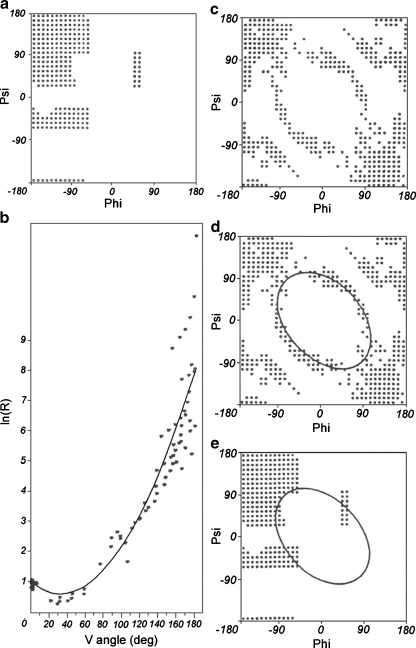
determines the optimal path on the Ramachandran map considered the complete conformational space. The elliptical path on the Phi-Psi map links the locations of all secondary structures. This path is assumed to represent the limited conformational sub-space available for the backbone in the ES step of the folding process. The agreement between the model and the protein is estimated by calculating the average distance (D average) between the projected value of the radius of curvature and the one observed one for the appropriate V-angle value as it appears for particular residue in the polypeptide chain. The graphic interpretation of the ES model is given in Fig. 1.
Fig. 1.
The ES model definition. (a) the Ramachandran map with low energy area distinguished (b) the relation between V-angle (dihedral angle between two sequential peptide bond planes) and R – radius of curvature (in logarithmic scale to avoid large values for β-structural forms) as calculated for structures belonging to low energy fragments on Ramachandran map (shown in a) together with the approximation function (2nd degree polynomial). (c) the Ramachandran map with points representing the structures accordant with the approximation function shown in b). (d) the ellipse path assumed to represent the limited conformational sub-space for early-stage intermediate. (e) the ellipse path linking all secondary structures area
Late stage model
The tertiary structure of the protein in the LS step of the protein folding process as assumed to be reached during the generation of the hydrophobic core with a simultaneous optimization of all other non-bonding interactions (electrostatic, vdW and torsional potential). The presence of an external force field is expressed via the three-dimensional Gauss function [17]. Model extends the original one introduced by Kauzman [18]. The force field simulates the hydrophobic core of the “fuzzy oil drop” model with the highest concentration of hydrophobicity in the center of the ellipsoid with its decrease depending on the distance from the center of the ellipsoid and the concentration reaching zero on the surface of the “drop”, according to the Gauss function:
 |
2 |
where  are the coordinates of the geometric center of the molecule (usually located in the origin of the coordinate system). This is why these values can be considered equal to zero. The size of the molecule is expressed by the triple σx, σy, σz, which is calculated for each molecule individually provided that the orientation of the molecule with the longest possible inter-effective atoms distance is determined according to the appropriate coordinate system axis. The σ values are calculated as 1/3 of the longest distance between two effective atoms calculated along each axis. The value of the Gauss function at any point of protein body is treated as the idealized hydrophobic density defining the hydrophobic core.
The idealized hydrophobicity at any point of the “fuzzy oil drop” can be calculated according to the Gauss function for the molecule located with its geometric center as the origin of the coordinate system. On the other hand, the empirical hydrophobicity distribution is calculated according to the function presented by Levitt [19].
 |
3 |
where N expresses the number of amino acids in the protein (number of grid points),  expresses the hydrophobicity of the ith residue according to the accepted hydrophobicity scale (the Aboderin scale was applied in this work [20]), r
ij expresses the distance between the i-th and j-th interacting residues, and c expresses the cutoff distance, which according to the original paper [19] is assumed to be 9 Å. The values of
  are standardized by dividing them by the coefficient
  , which is the sum of all hydrophobicities attributed to grid points.
Hydrophobicity distribution in the molecule under consideration appeared to be highly consistent with the idealized one. However, the irregularities observed in many proteins appeared to be target-oriented and related to active sites, such as ligand binding sites or enzymatic active sites.
Kullback-Leibler information entropy
The accordance between the idealized and the observed hydrophobicity distribution is measured according to the Kullback-Leibler relative (divergence) entropy [21], which quantifies the distance between two distributions. The distance between the observed and the theoretical (O/T) distribution was calculated. This value can be estimated only with respect to other solutions. The random distribution of hydrophobicity represented the border case for which the distance (O/R) was calculated. The relation O/T < O/R was taken as evidence for a non-random distribution close to theoretical one.
 |
4 |
where: D KL – distance entropy, p – probability of a particular observed event, p 0 – probability in reference distribution. The index “i” denotes a particular amino acid. N denotes the number of amino acids in the polypeptide chain.
Results
The structural analysis of the mutants is performed in respect to the ES and LS structural characteristics using the VR model and “fuzzy oil drop” model with the distance entropy applied to quantitative measurements of the structural differences between two structures under consideration.
Structural analysis of proteins under consideration
A structural analysis of proteins under consideration with respect to the ES and LS is presented in Table 1.
Table 1.
The ES and LS characteristics of proteins under consideration. The position of mutations is given in the second column, followed by the value of D (distance), which is a measure of the accordance with the adopted model of ES intermediate. The D average expresses the mean distance between the projected and observed values of parameters that describe the structure of ES intermediate. The proteins with D average values below 1.0 are considered consistent with the ES model. The protein of the relation O/T < O/R is interpreted as accordant with LS model O/T denotes the Kullback-Leibler entropy calculated for the observed (O) distribution of hydrophobicity density and theoretical one (T) treated as the target distribution in comparison with the O/R expressing the distance between observed one and random (R) treated as the target distribution. Chains A were taken for analysis in NMR technique determining the protein structure. The values given in bold denote the case of accordance with appropriate model
| PDB - ID | Mutation | D average | O/T | O/L |
|---|---|---|---|---|
| 1AME | P64A, P65A | 1.214 | 0.058 | 0.066 |
| 2AME | P64A, P65A, N14Q | 1.174 | 0.062 | 0.072 |
| 3AME | P64A, P65A, Q9T, Q44T | 1.102 | 0.055 | 0.060 |
| 4AME | P64A, P65A, T18A | 1.164 | 0.061 | 0.066 |
| 6AME | P64A, P65A, M21A | 1.202 | 0.059 | 0.069 |
| 7AME | P64A, P65A, T15A | 1.354 | 0.058 | 0.067 |
| 8AME | P64A, P65A, N14S, A16H | 1.251 | 0.059 | 0.066 |
| 9AME | P64A, P65A, S42G | 1.403 | 0.060 | 0.068 |
| 1MSI | P64A, P65A | 1.190 | 0.065 | 0.066 |
| 2MSI | A16M | 1.251 | 0.080 | 0.062 |
| 3MSI | A16H | 1.334 | 0.077 | 0.059 |
| 4MSI | A16T | 1.396 | 0.068 | 0.061 |
| 5MSI | A16C | 1.318 | 0.071 | 0.061 |
| 6MSI | A16R | 1.303 | 0.067 | 0.057 |
| 7MSI | A16Y | 1.294 | 0.066 | 0.060 |
| 8MSI | P64A, P65A, N14S, Q44T | 1.192 | 0.056 | 0.062 |
| 9MSI | P64A, P65A, T18N | 1.238 | 0.054 | 0.062 |
| 1MSJ | P64A, P65A, T15V | 1.237 | 0.060 | 0.068 |
| 2MSJ | P64A, P65A, N46S | 1.163 | 0.058 | 0.064 |
| 1JAB | P64A, P65A, T18A | 1.153 | 0.058 | 0.067 |
| 1JIA | P64A, P65A, K61I | 1.213 | 0.060 | 0.064 |
| 1B7I | P64A, P65A, K61R | 1.275 | 0.055 | 0.063 |
| 1B7J | P64A, P65A, V20A | 1.273 | 0.057 | 0.067 |
| 1B7K | P64A, P65A, R47H | 1.315 | 0.055 | 0.066 |
| 1KDE | INS(M0) P64A, P65A, INS(K66, D67, E68, L69) | 1.113 | 0.061 | 0.091 |
| 1KDF | INS(M0) P64A, P65A, INS(K66, D67, E68, L69) | 0.989 | 0.059 | 0.076 |
| 2SPG | T15S | 1.381 | 0.060 | 0.067 |
| 1J5B | T(2,13,24,35)V A(7,29)K, A(11,33)E | 0.192 | 0.349 | 0.072 |
Applicability of the ES model
According to the ES model, structure is generated according to backbone preferences in terms of the V-angle and R-radius of curvature. This is why the values of V-angle and R-radius of curvature (in logarithmic units) as they appear in the crystal structures of proteins under consideration were analyzed versus the idealized curve. The D distance between the projected and observed values of parameters was calculated. It was arbitrarily assumed that proteins with average D below 1 exhibit a structure consistent with the model. However, in view of the availability of the final (LS stage) structures, a D average value above 1 does not imply that the model is inadequate. A low value of D suggests that the structural elements characteristic of the ES structural form have been preserved to a large degree in native (LS structure). All helical fragments are present in both the ES and the LS. That is why low values of D average may suggest a large participation of secondary structures of the helical type.
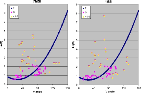
Two proteins representing extreme cases (large and low D values) are shown as examples in Fig. 2. The distribution of the observed values (V, ln(R)) in comparison to the idealized approximation curve is shown in Fig. 2.
Fig. 2.
The ES model applicability to 7MSI and 1MSI – proteins of lower and higher (respectively) discordance with the assumed model although both of them are treated as representing the structure not accordant with the ES model (Daverage above 1.). The dark blue symbols – theoretical dependence between V-angle and Ln(R), pink squares – observed parameters and yellow triangles – the residues of the higher than 1.0 unit difference between expected and observed values of ln(R) for particular V-angle
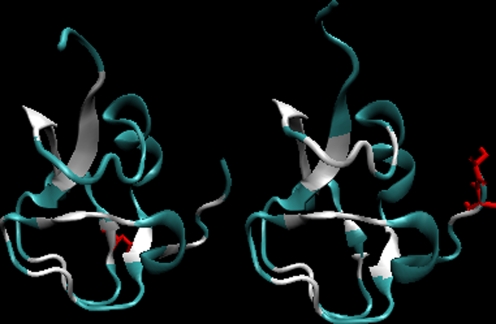
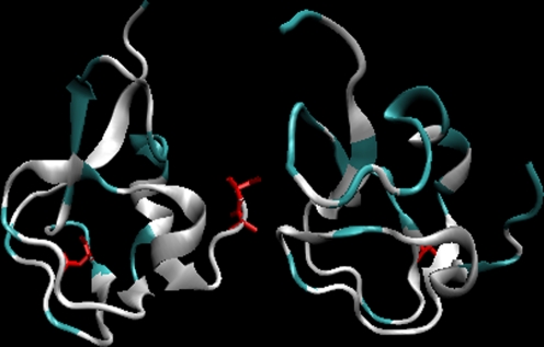
The 3-D structures with residues with D average above 1 are marked in red in this picture in order to visualize the character of the structural motif which is not consistent with the adopted model (Fig. 3).
Fig. 3.
The 3-D presentation of the 7MSI (left) and 1MSI (right) proteins differing their lower and higher (respectively) accordance with the LS model. The fragments marked in white – residues of difference higher than 1.0 unit shown in Fig. 1 as yellow triangles. The residues shown in red – mutations versus the wild type
The accordance of the crystal structure with the ES model is not typically expected. On the other hand, the crystal structure is usually consistent with the LS model, the ES to LS transition is the change of optimal backbone conformation toward the presence of a hydrophobic core. Thus, it is obvious that ES characteristics may be lost in the LS intermediate, although this is not always the case. 1J5B is the only example among the discussed antifreeze proteins (type I). Its structure is entirely helical, and appears to be highly consistent with the ES model. The distribution of hydrophobicity in this molecule is much closer to the random distribution than to the Gaussian one.
Applicability of the LS model
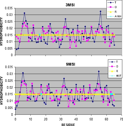
The LS model assumes that hydrophobicity distribution in the protein molecule is consistent with the idealized one, expressed by the three-dimensional Gauss function. The profile showing the hydrophobic interactions collected by effective atoms of each residue as the effect of interactions with other amino acids is shown in Fig. 4.
Fig. 4.
The hydrophobic density profile for 3MSI and 9MSI showing the idealized and observed distributions. The proteins were selected to show the lowest and the highest respectively accordance between the idealized (T) and observed (O) hydrophobicity distribution. The yellow line shows the random distribution (R). The residues mutated versus the wild type are shown by cyan circles
The 3-D presentation of protein molecules with residues (marked in white) with strongest hydrophobic interactions (responsible for the generation of the hydrophobic core) in two proteins selected to represent the best and the worst accordance with the model under consideration is shown in Fig. 5.
Fig. 5.
3-D presentation of 3MSI (left) and 9MSI (right) with the residues of hydrophobicity density differing more than 0.004 versus the expected one given in white. The residues shown in red – the mutated residues
The Kullback-Leibler distance entropy
The accordance between the observed and the idealized hydrophobic density distributions was expressed quantitatively using the Kullback-Leibler distance entropy (as shown in Materials and methods). The values measuring the distance between the observed and idealized (O/T) and the observed and the random (O/R) distributions are given in Table 1. The analysis of these values suggests that the structural changes do not influence the status of the structure (accordance with the idealized model is preserved). Some proteins undergo changes that result in structure no longer consistent with the adopted model, which suggests that the mutations destroy the hydrophobic core responsible for stabilizing the molecule.
A particular mutation in position 16 in 2MSI to 7MSI in respect to 1MSI appeared to affect the hydrophobic core to such a large extent that it lost its initial structure and became inconsistent with the idealized core structure.
Substituting Pro in positions 64 and 65 with Ala, which is absent in the other investigated proteins and their mutants, suggests that prolines play a critical role as far as hydrophobic core generation is concerned.
The investigated molecules are classified in Table 2 depending on accordance with ES and LS models.
Table 2.
Protein classification with respect to the criteria describing/defining the early stage (ES) and late stage (LS) intermediates
| ES model | |||
|---|---|---|---|
| Consistent | Non-consistent | ||
| LS model | Consistent | 1KDF | 1AME, 2AME, 3AME, 4AME, 6AME, 7AME, 8AME, 9AME, 1KDE, 1MSI, 8MSI, 9MSI, 1MSJ, 2MSJ, 2SPG, 1JIA, 1JAB, 1B7I, 1B7J, 1B7K |
| Non-consistent | 1J5B (I) | 2MSI, 3MSI, 4MSI, 5MSI | |
The majority of the proteins under consideration are very similar (both in terms of sequence and structure), there is only one (1KDF – minimized averaged NMR structure) that satisfies the conditions of both models (ES and LS). This may suggest that the initial ES intermediate was not destroyed in the transition to LS.
The accordance with the LS model is the strongest one in 1KDE structure. The structural fluctuation of dynamic forms seems to be limited by the stabilization imposed by the hydrophobic core (in accordance with the three-dimensional Gauss function).
On the other hand, its four mutants (2MSI, 3MSI, 4MSI, 5MSI) are examples in which mutation prevented the formation of hydrophobic core, which is present in all other structural forms of other mutants of this protein.
Structural differences in pair-wise comparison
A comparison of the intensity of structural changes upon mutation in relation to other proteins of the same group is shown in Table 3. Such a ranking allows contrastive analysis, even more significantly so in this case due to identical (or similar) polypeptide chain length.
Table 3.
Pair-wise comparison of selected mutants (AMI). The values under the diagonal – the RMS-D measurements: the values above the diagonal present the D KL distance entropy between two proteins (according to the column and row headers)
| D KL | |||||||||
|---|---|---|---|---|---|---|---|---|---|
| AMI1 | AMI2 | AMI3 | AMI4 | AMI6 | AMI7 | AMI8 | AMI9 | ||
| RMS-D | AMI1 | 0.294 | 0.196 | 0.201 | 0.250 | 0.315 | 0.294 | 0.265 | |
| AMI2 | 0.080 | 0.267 | 0.200 | 0.204 | 0.150 | 0.142 | 0.178 | ||
| AMI3 | 0.078 | 0.128 | 0.162 | 0.208 | 0.292 | 0.276 | 0.227 | ||
| AMI4 | 0.049 | 0.095 | 0.074 | 0.162 | 0.237 | 0.213 | 0.168 | ||
| AMI6 | 0.082 | 0.046 | 0.122 | 0.093 | 0.240 | 0.244 | 0.199 | ||
| AMI7 | 0.056 | 0.088 | 0.088 | 0.058 | 0.084 | 0.147 | 0.226 | ||
| AMI8 | 0.056 | 0.090 | 0.096 | 0.066 | 0.084 | 0.051 | 0.198 | ||
| AMI9 | 0.054 | 0.099 | 0.082 | 0.055 | 0.098 | 0.062 | 0.073 | ||
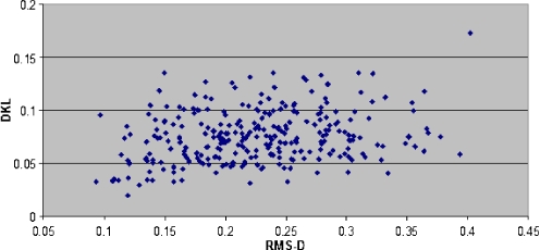
The LS model based comparative structural analysis was performed using the Kullback-Leibler divergence entropy treating one of the compared proteins as the target. The values received on the basis of these calculations were compared with traditionally used similarity scale expressed by RMS-D values. The appropriate values for selected mutants (group AMI) are given in Table 3.
The correction coefficient for D KL versus RMS-D as calculated using STATISTICA program is equal 0.2268 with p < 0.0001. The graphic presentation of this relation is shown in Fig. 6.
Fig. 6.
The relation between traditional similarity measurements expressed as RMS-D values and D KL measurements. The correlation coefficient calculated is equal to 0.2268 with the statistical significance on the level p < 0.0001
Conclusions
The molecules presented in this paper are examples of proteins with structure which seems to satisfy the adopted model of “fuzzy oil drop”. When folding, these molecules satisfy all the conditions defined by non-bonding interactions with simultaneous hydrophobic core formation. Hydrophobic residues located in the central part of the molecule and exposure of hydrophilic residues on the surface are the main tenets of the “oil drop” model introduced by Kauzmann [18]. The Kullback-Leibler entropy [21], which is a measure of the distance between the target distribution (idealized one) and the one observed in a particular molecule revealed good accordance of the observed hydrophobicity distribution with the idealized one.
The Kullback-Leibler entropy calculated for different mutants seems to quantitatively express the scale of structural differences in terms of the hydrophobic core structure.
The selected proteins are examples supporting the reliability of the “fuzzy-oil-drop” model. This model reproduces/imitates the mechanism of protein folding. The modification of the “fuzzy oil drop” model for proteins that are not consistent with this model is under consideration.
The loss of the accordance with the ES model in the LS step of protein folding is obvious, although some proteins with highly preserved secondary structures also exhibit this accordance in their late stage structural form.
It is difficult to verify the applicability of the presented model with respect to biological activity of the proteins under consideration. Their biological function requires high solubility, but no specific interactions understood as necessary formation of binding sites. The antifreeze proteins interact non-specifically and their role is to neutralize water’s tendency to be highly organized. The exposure of poorly hydrophobic (i.e., hydrophilic) residues on the protein surface very likely ensures such an effect.
The application of the presented model to the proteins with well-defined active sites may also reveal its ability to locate them. When used for mutants it may estimate the influence of mutation on the potential loss of biological activity [22]. The position of mutation and its relation to the location of residues engaged in biological function may easily be visualized when the  profile is presented (
 expresses the difference between expected and observed hydrophobicity revealing the residues of significant difference between observation and the model). Such an analysis was presented in [22].
The influence of mutation on the structure and, subsequently, on biological activity was defined using the hydrophobic density distribution.
When hydrophobicity distribution in the protein molecule is consistent with the idealized one, the protein molecule exhibits high solubility, but no specific biological activity. It had been assumed in the past that such proteins with no biological function do not exist. However, the antifreeze proteins appeared to satisfy the above-mentioned conditions. That is why proteins from this group were selected as examples to visualize different forms of the accordance between the assumed model and the real structure in antifreeze proteins.
The pair-wise differences for mutants appeared of much higher magnitude in terms of the relation between the idealized and observed hydrophobicity distributions.
The opposite situation is observed in the group of peroxidases, where the pair-wise comparison reveals far smaller differences.
This paper was focused on good applicability of the Kullback-Leibler entropy as a measure of distance between two distributions.
This method is very simple and it seems to be a suitable tool for automatic analysis of large amounts of data (structures of mutants and/or structures of proteins with equal numbers of amino acids in polypeptide chains).
The protein 3BDN was taken to estimate the applicability to the larger proteins (above 200 amino acids) [23].
The applicability of Kullback-Leibler entropy for the set of proteins belonging to the antifreeze proteins revealed the high accordance of the structure characteristics of this group of proteins with the “fuzzy oil drop” model. It suggests that the hydrophobic core in proteins under consideration represents the structure (hydrophobic density distribution) of three-dimensional Gauss function. The consequence of this observation is that the presence of external force field in folding process simulation may be treated as the heuristic model for protein folding simulation. The other group of proteins were also recognized as proteins of structure in accordance with “fuzzy oil drop” model. They are: fast folding proteins, cold shock proteins and some proteins in the form of homodimers (currently under consideration). The protein of the structure assumed to represent the early stage step of folding process and its native structural form appeared to be well accordant with both ES and LS mode respectively [24]. The “fuzzy oil drop” model is able to explain the structural differentiation of two homologous proteins of significantly different structure (change of α-helix to the β-structural form). Although all proteins listed as accordant with the “fuzzy oil drop” model are of the category “easy predictable” (according to CASP classification [25]) the meaning of the presented model is its general character. The introduction of external force field and the accordance of structures of some proteins with the model suggests the significant role of the environment for folding process.
Acknowledgments
This work was financially supported by Jagiellonian University – Medical College - Grant No K/ZDS/001531.
Open Access
This article is distributed under the terms of the Creative Commons Attribution Noncommercial License which permits any noncommercial use, distribution, and reproduction in any medium, provided the original author(s) and source are credited.
References
- 1.Hari SB, Byeon C, Lavinder JJ, Magliery T. Protein Sci. 2010;19:670–679. doi: 10.1002/pro.342. [DOI] [PMC free article] [PubMed] [Google Scholar]
- 2.Yagawa K, Yamano K, Oguro T, Maeda M, Sato T, Momose T, Kawano S, Endo T. Protein Sci. 2010;19:693–702. doi: 10.1002/pro.346. [DOI] [PMC free article] [PubMed] [Google Scholar]
- 3.Chung HS, Shandiz A, Sosnick TR, Tokmakoff A. Biochemistry. 2008;47:13870–1387. doi: 10.1021/bi801603e. [DOI] [PMC free article] [PubMed] [Google Scholar]
- 4.Sapra KT, Balasubramanian GP, Labudde D, Bowie JU, Muller DJ. J Mol Biol. 2007;376:1076–1090. doi: 10.1016/j.jmb.2007.12.027. [DOI] [PMC free article] [PubMed] [Google Scholar]
- 5.Couñago R, Wilson CJ, Peña MI, Wittung-Stafshede P, Shamoo Y. Protein Eng Des Sel. 2008;21:19–27. doi: 10.1093/protein/gzm072. [DOI] [PubMed] [Google Scholar]
- 6.Kurpiewska K, Font J, Ribó M, Vilanova M, Lewiński K. Proteins. 2009;77:658–669. doi: 10.1002/prot.22480. [DOI] [PubMed] [Google Scholar]
- 7.Lonquety M, Lacroix Z, Papandreou N, Chomilier J, Lonquety M, Lacroix Z, Papandreou Z, Chomilier J. Nucleic Acids Res. 2004;37:D374–D379. doi: 10.1093/nar/gkn704. [DOI] [PMC free article] [PubMed] [Google Scholar]
- 8.Fernández M, Caballero J, Fernández L, Abreu JI, Acosta G. Proteins. 2008;70:167–175. doi: 10.1002/prot.21524. [DOI] [PubMed] [Google Scholar]
- 9.Capriotti E, Fariselli P, Casadio R. Nucleic Acids Res. 2005;33:W306–W310. doi: 10.1093/nar/gki375. [DOI] [PMC free article] [PubMed] [Google Scholar]
- 10.Karchin R, Kelly L, Sali A. Pac Symp Biocomput. 2005;2005:397–408. doi: 10.1142/9789812702456_0038. [DOI] [PubMed] [Google Scholar]
- 11.Fernández L, Caballero J, Abreu JI, Fernández M. Proteins. 2007;67:834–852. doi: 10.1002/prot.21349. [DOI] [PubMed] [Google Scholar]
- 12.Hoekstra HE, Coyne JA. Evolution. 2007;61:995–1016. doi: 10.1111/j.1558-5646.2007.00105.x. [DOI] [PubMed] [Google Scholar]
- 13.Christ D, Winter G. Proc Natl Acad Sci USA. 2003;100:13202–13206. doi: 10.1073/pnas.2134365100. [DOI] [PMC free article] [PubMed] [Google Scholar]
- 14.Roterman I, Brylinski M, Konieczny L, Jurkowski W. In: Recent advances in structural biology. de Brevern AG, editor. Trivandrum: Research Signpost; 2007. [Google Scholar]
- 15.Roterman I (2009) Structure-function relation in proteins. Transworld Research Network T.C. 37/661(2), Fort P.O. Trivandrum, Kerala, India
- 16.Roterman I. J Theor Biol. 1995;77:283–288. doi: 10.1006/jtbi.1995.0245. [DOI] [PubMed] [Google Scholar]
- 17.Konieczny L, Brylinski M, Roterman I. In Silico Biol. 2006;6:15–22. [PubMed] [Google Scholar]
- 18.Kauzmann W. Adv Protein Chem. 1959;14:1–63. doi: 10.1016/S0065-3233(08)60608-7. [DOI] [PubMed] [Google Scholar]
- 19.Levitt M. J Mol Biol. 1976;104:59–107. doi: 10.1016/0022-2836(76)90004-8. [DOI] [PubMed] [Google Scholar]
- 20.Aboderin A. Int J Biochem. 1971;2:537–544. doi: 10.1016/0020-711X(71)90023-1. [DOI] [Google Scholar]
- 21.Nalewajski RF. Information theory of molecular systems. Amsterdam: Elsevier; 2006. [Google Scholar]
- 22.Prymula K, Sałapa K, Roterman I. J Mol Model. 2010;16:1269–1282. doi: 10.1007/s00894-009-0639-2. [DOI] [PubMed] [Google Scholar]
- 23.Stayrook SE, Jaru-Ampornpan P, Ni J, Hochschild A, Lewis M. Nature. 2008;452:1022–1025. doi: 10.1038/nature06831. [DOI] [PubMed] [Google Scholar]
- 24.Religa TL, Markson JS, Mayor U, Freund SM, Fersht AR. Nature. 2005;37:1053–1056. doi: 10.1038/nature04054. [DOI] [PubMed] [Google Scholar]
- 25.Orengo CA, Bray JE, Hubbard T, LoConte L, Sillitoe I. Proteins Suppl. 1999;3:149–170. doi: 10.1002/(SICI)1097-0134(1999)37:3+<149::AID-PROT20>3.0.CO;2-H. [DOI] [PubMed] [Google Scholar]


