

Abstract
Direct infusions into brain parenchyma of biological therapeutics for serious brain diseases have been, and are being, considered. However, individual brains, as well as distinct cytoarchitectural regions within brains, vary in their response to fluid flow and pressure. Further, the tissue responds dynamically to these stimuli, requiring a nonlinear treatment of equations that would describe fluid flow and drug transport in brain. We here report in detail on an individual–specific model and a comparison of its prediction with simulations for living porcine brains. Two critical features we introduced into our model — absent from previous ones, but requirements for any useful simulation — are the infusion-induced interstitial expansion and the backflow. These are significant determinants of the flow. Another feature of our treatment is the use of cross–property relations to obtain individual–specific parameters that are coefficients in the equations. The quantitative results are at least encouraging, showing a high fraction of overlap between the computed and measured volumes of distribution of a tracer molecule, and are potentially clinically useful. Several improvements are called for; principally a treatment of the interstitial expansion more fundamentally based on poroelasticity, and a better delineation of the diffusion tensor of a particle confined to the interstitial spaces.
1. Introduction
The blood–brain barrier (BBB) has been a core obstacle in getting otherwise promising therapies into the central nervous system, even for small molecules [30]. Many methods for overcoming this barrier have been proposed and tried. One of these is the subject of this paper: the direct insertion of a catheter into the brain parenchyma followed by pressure-driven infusion of a solution containing the therapy. The use of this was pioneered by researchers at the NIH [27], and called by them convection–enhanced delivery (CED). It has been almost two decades since this method was proposed and explored, and yet it still has not found its way to clinical practice, though there is a very large number of papers that report on its performance, and advocate its use. The NIH group which pioneered the method, has been prolific in this area [24], [26], [9], [25], [12]. Almost a decade ago, we proposed a method that could be used to predict the distribution of infusate delivered thus in an individual brain [34], i.e., specific to the anatomy and physiology of the brain of the individual. The motivation was that, owing to the large spatial heterogeneity of a brain, and the large variation amongst different brains even in a single species, it would be useful to have such a simulation to plan the placement of catheters, and delivery of the infusate.
This paper has one principal purpose: to report in detail upon our first individual-specific simulation. Accordingly, apart from this Introduction and the Conclusions, the paper is divided into two major sections: (a) one that describes the model and methods used and (b) the following one that compares it quantitatively with in-vivo data obtained in a pig brain. Prior work in each of the areas required to develop and implement our model is discussed at the end of each of the respective sections. The Conclusions point out improvements to be aimed for in both the data collection and the model. The actual protocol used and a descriptive exposition of some of the results obtained from the experiments has already appeared in [6] and so we shall be quite brief on this.
2. Interstitial transport model
In this section we describe first (i) the equations that define the model, next the (ii) the in-vivo imaging or other assumptions we use to fix these parameters in the equations, and finally (iii) the methods we use to solve the equations.
2.1. Equations
We use a standard mathematical framework for drug distribution in CED, as for example in [27]. In this, the drug concentration, c(x, t) has to be solved for as a function of spatial distribution in brain parenchyma (x) and time t. The equation for its rate of change with time is approximated as a sum of (i) diffusion, (ii) changes due to bulk flow driven by convection and (iii) losses due to movement out of parenchyma and to metabolism. These three mechanisms correspond to the three terms on the right hand side of equation (1):
| (1) |
ϕ is the volume fraction of the interstitial spaces to which the moving particle is restricted, and ϕc is the concentration of the particle in question (drug, or, in this study, the MR contrast agent) measured per unit volume of tissue. The pseudo-velocity v denotes the volume of fluid per unit time traversing a unit area in tissue situated normal to the direction of the vector v. Due to the fact that we can associate a vector normal to an area element in three dimensions, this velocity may be considered a vector, more properly a co-vector in mathematical terminology.
 is the diffusion tensor of the particle restricted to the tortuous interstitium outside of the cells. k is a linear approximation of the rate constant of loss of drug through a volume distribution of sinks to account for both the irreversible metabolism losses and disappearance through capillaries. (We can lump these two contributions together as long as we linearize.) ϕ is the fraction of volume occupied by the interstitium, assumed to be a connected space. We assume diffusion obeys Fick's law (see [41] for discussion of greater depth on this point).
To specify equation (1) precisely, we need to know ϕ, v,
, k as functions of x. (As will be seen we will simplify the problem so that they are not functions of time, i.e., they refer to the steady state.) The solvent fluid velocity v is computed via Darcy's law,
| (2) |
which, together with fluid (non)conservation within the volume:
| (3) |
(the symbol such as ≕ above means that the quantity facing the colon is defined to be the quantity facing the equals sign) gives, by substituting (2) in (3):
| (4) |
In these equations, p is interstitial pressure relative to the background interstitial pressure (the Starling pressure, see [28]), Lp is the capillary hydraulic conductivity governing the rate of net flow of water across capillary membranes and
is the capillary area per unit tissue volume.
 is the extracellular hydraulic conductivity tensor of tissue. The three sets of equations (1),(2),(4) form a closed system to solve for the concentration if we know the boundary conditions and also the scalar parameters ϕ, k, α, and the tensor ones
and
. We emphasize that all these quantities until further notice are fields, i.e., are, in general, inhomogenous with different values in different portions of brain.
is the extracellular hydraulic conductivity tensor of tissue. The three sets of equations (1),(2),(4) form a closed system to solve for the concentration if we know the boundary conditions and also the scalar parameters ϕ, k, α, and the tensor ones
and
. We emphasize that all these quantities until further notice are fields, i.e., are, in general, inhomogenous with different values in different portions of brain.
Inevitably, before describing how we obtain these scalar and tensor fields for an individual, we need to reduce the equations still further to obtain for a tractable set to solve. We carefully discuss the assumptions already inherent in the equations, and the phenomena we cannot neglect. These allow us to offer truncations to reduce these to the steady state so we can proceed with a simpler theory.
2.1.1. Assumptions
Many possible complications have been neglected that may pertain to active therapeutic molecules. The principal ones are (i) equation (1) neglects chemical kinetics which would result in a nonlinearity in the final term on the right. In this stage of investigation, it is more important to see how far a drug molecule can travel than to get its concentration exactly right, so we assume that the concentration is high enough that the second or higher order kinetics of chemical reactions may be neglected. The tracer used in our studies of course has no chemical reactions during infusion so this assumption is perfectly good for the results here. (ii) The routes for particle transport have been assumed to be within the interstitial space so that axonal transport [11], [18] or physical adsorption [7] at the interface between tissue and extracellular space are both neglected. (iii) v is an effective velocity of advection of the particle by the fluid. In the numerical simulations reported on in this paper, we set this to be the velocity of the fluid (solvent) that is infused, and so use the same symbol for both. Our assumption that the solute is freely advected with the fluid is less likely to be true for large or charged particles, or those much more dense than the fluid. Often the advective velocity is written as the the fluid velocity multiplied by a number less than one, called the retardation factor. However, the molecule tracked here is small (less than 5 nm in diameter), and the interstitial widths are reported to be at least 10 times larger than that [48] so there is no strong reason to doubt full advection. Of course, comparing the measured and computed distributions does offer an indirect check of this assumption. (iv) Although our simulations allow for hydrodynamic dispersion, which is a correction from the averaged Darcy flow to account for the tortuous interstitial pathways (see [4]), the results reported below do not include this, for simplicity.
Continuing, equation (3) assumes (v) there is no variation in resting pressure (here set to zero) within brain tissue in the absence of infusion, (vi) there is no endogenous flow in the absence of infusion, and (vii) that the plasma proteins don't make their way into the interstitium. Note that these assumptions don't need to hold exactly but only that the neglected phenomena result in negligible impact within the spatiotemporal scales of the experiment. For example, we know that even when there is no infusion (so that we assume p = 0), there is still production of interstitial fluid coming from the capillaries and absorbed in the ventricles and boundaries of the cerebrospinal fluid (CSF). However, the rate of this endogenous flow is slow enough (< 0.1μ L / min / gm [1]) that we here neglect the correction it would require for the resting interstitial pressure in brain. Equally though, our assumptions would not be correct for a significantly disrupted BBB, such as is present in a brain with an active tumor. There is evidence that the introduction of a catheter itself causes such significant disruption in its vicinity [20], a phenomenon we do not explicitly include in the simulations we will report upon here. Finally, (viii) we assume here that the infusate has been treated to have the same effective viscosity as the interstitial fluid with no immiscibility or viscous fingering effects, and that the fluid is Newtonian [16]. Also, (viii) any osmolarity or oncotic effects due to the infusate [8] are neglected. We shall always assume that the solution infused is iso-osmolar with the fluid in the interstitial space. Finally, (ix), bubbles are banned! If the infusion procedure allows ready formation of air bubbles in tissue, their size and presence will be unpredictable, along with how they affect the fluid flow. It is assumed that the device, system, and protocol prevent this from happening.
2.1.2. Brain edema, deformation and poroelasticity
Having satisfied ourselves that the equations we have written down may be a good enough set to describe infusate distributions we must confront the fact that the brain is far from a rigid porous medium: not only is it visibly and literally palpably pulsatile with the heartbeat, it has long been known that it is edematous under various disease and trauma conditions. These arise out of the interaction of fluid flow and the elasticity of the tissue which means also that the general framework to model these is time-dependent poroelasticity, more generally, visco-poro-elasticity. This results, in general, with quantities such as the fluid pressure or interstitial fraction becoming both time-dependent and coupled to the degrees of freedom of the solid tissue framework. Poroelasticity itself is treated in a number of texts [52], [10], and in the context of the brain, for hydrocephalus (see e.g., [42], [43], [46] for a small sampling). Our approach to this problem is in steps. In this paper, we shall describe the phenomena by a steady state model (avoiding the complication of dealing with time dependence) and further describing only the fluid degrees of freedom, and not those of the porous solid frame (thus avoiding coupled fluid–solid interaction). Obviously, this truncation of the poroelastic theory is an approximation that is only as good as the results it generates. However, this reduction is well motivated: what is most pertinent to the experiments used in this paper are two important effects that we highlight: (i) infusion–induced edema and (ii) backflow along the outer surface of the catheter. We now describe these.
2.1.2.1. Interstitial expansion and determination of ϕ
Expansion of the interstitial space can be very significant [6], [53], which in turn implies significant changes in hydraulic conductivity (factors of 10 and more). To predict this expansion from infusion– generated edema somewhat rigorously we would have to resort to poroelasticity theory. We are immediately faced with a dilemma. While we must account for differences in expandability in different cytoarchitectural regions (white versus gray matter), we also expect that the expansion will, in general, be anisotropic. For example the major white matter tracts spread apart very readily, but are not elongated. This requires us to introduce tensors into the constitutive relations; for example in a linear approximation, the strain (second rank tensor), which indicates how the porous tissue frame expands, will depend on the fluid pressure through a second rank tensor as well. We want to severely restrict the growth of parameters in the model! In the experiments reported on here, the infusions were directly into the white matter of the internal capsule, and the expansion remained highly localized to the white matter, with little observed change in gray matter regions. Further, we assume for the moment that the initial lateral spread of the fibers happens as if the fibers were simply suspended in fluid, consistent with the easy expandability. This then saturates at an upper value (see below) of the interstitial volume fraction, presumably when the cross–linking of the fibers becomes taut. We estimate this interstitial fraction expansion everywhere, as if the infusion covered the entire brain. This will be incorrect where there is no infusate, but there will be no infusion simulation at these locations anyway. For our purposes, namely to replace the complexity of dynamic poroelasticity with a quasistatic change of interstitial fraction and subsequent rigid porous medium behavior, we feel this is a good starting point. Thus, the interstitial fraction change corresponds to a correction for edema covering the entire brain. The estimation is done as follows, at every voxel in the imaging volume.
1. We assign the resting interstitial volume fraction to be 0.2 throughout the brain following [45].
2. We then estimate the fraction of unexpanded white matter fWM contained in the voxel. We have done this in an ad hoc fashion, using the fractional anisotropy F A of the diffusion tensor computed in a standard way [3], and then setting
| (5) |
which yields a white matter fraction of 0.5 when FA = FAmax/2. On either side of this value, fWM heads asymptotically towards 0 or 1. The parameter s determines the steepness of the approach. We have used s = 20, and FAmax = 0.45. The simulation results are not very sensitive to these parameters: their only function is to have a steep yet smooth dependence of the white matter fraction to the fractional anisotropy.
3. Finally, we modify the local interstitial fraction by changing the unexpanded white matter to the maximum expanded interstitial fraction value, ϕmax and interpolating linearly between the original and the maximum fraction allowed:
| (6) |
We use ϕmax = 0.45 in pigs simply because we obtained the best results with this value: this is further discussed in the Results section. (For simulations in humans, we use a larger value of 0.6 for this quantity.) We emphasize that our discussion on edema has been confined to ‘benign’ edema: the conditions that pertain when the intracerebral pressure begins to rise dangerously – important as these are in the management of brain cancer – are outside the scope of the present work. So, in our simulations the pressure in the CSF regions remains at the pre-infusion values, and is considered the fiducial pressure, set to zero. We note that in the approximation used here, the expansion depends on neither the fluid pressure increase nor on the actual increment of fluid content in the representative volume, as it should in a more proper treatment. We should also point out that since reducing the diffusion weighted signals to form a symmetric tensor means that directional fibers are indistinguishable within a voxel from crossing fibers, the genu of the corpus callosum also appears with high fractional anisotropy. Hence in our model, it will appear incorrectly as easily expandable. The reason that the genu does not expand easily has to do with the fibers crossing within it providing a tighter junction. While more sophisticated imaging methods such as diffusion spectrum imaging (DSI) can distinguish these crossings from the anisotropy of parallel fibers, DTI does not. If the infusion does not cross the midline, this will not cause a problem. However, if it does cross the midline, our model predicts expansion and higher conductivity within the genu, thereby altering the flow patterns within and beyond it. We shall later see a potential example of this in Figure 8. We are currently exploring a more fundamental approach using incremental poroelastic constitutive relations, which will also keep the white matter fraction from reaching too close to unity. The simulations reported here have used the above fitting procedure. The problem with a fuller poroelasticity model is that the number of parameters increases considerably, with the attendant problems of ascertaining their values in a living animal or human, and dependent on pathologies and individual variations.
Figure 8.
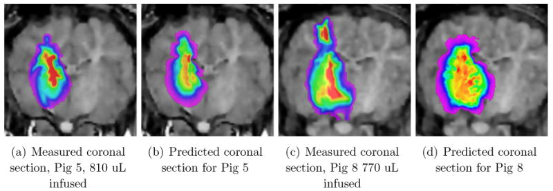
Distribution of infusate in a particular coronal section, for Pigs 5 and 8. The coronal section contains the catheter. Pig 5 is shown after 810 μL have been infused, while Pig 8 is shown after 770 μL of infusion. The distribution is significantly “fatter” in Pig 8, in this section, despite the smaller infused amount. Also, there seems to be a re-appearance of a higher concentration of infusate at the top of the brain in the measured distribution, absent in the predicted. This is discussed in the text.
The interstitial expansion modifies all the computations principally by requiring us to predict the changed hydraulic conductivity K that pertains. Our approach to hydraulic conductivity is via a cross-property relation, thus our treatment of
is addressed in the second subsection 2.2.
2.1.2.2. Backflow
Backflow is the result of competition between the water flow which proceeds best by pushing the tissue away so as to clear a channel between tissue and catheter, and the elasticity (shear modulus) of the tissue which pushes back and tries to close up to the catheter. We have extended a fundamental paper in this area [28] from the NIH, to obtain the extent of backflow, and the pressure and flow-rate variations along the catheter [33]. We quote below from our own work, which should be consulted for the derivation, to display the equations that determine steady state backflow that pertain to the single end–port type of catheter we have used in the porcine experiments. Let z be the distance along the catheter, with z starting at 0 at the catheter tip and increasing back along the catheter axis. Define Q(z) to be the flow rate in a tissue– free region adjacent to the catheter, and p(z) the corresponding pressure, both being defined essentially at the outer diameter of the catheter, rc, since the tissue–free region is extremely narrow. Let κ (z) and G (z) be similarly defined scalar (i.e., isotropic but usually inhomogeneous) tissue hydraulic conductivity and shear modulus, respectively. (For κ (z) we employ the trace of
, remembering to use the modification required by the interstitial expansion noted above.) Further let L denote a characteristic distance at which the pressure decreases to its resting value in the absence of infusion, roughly the distance of the outer limit of brain tissue from the catheter. Then define the hydraulic resistance as
| (7) |
Further define
| (8a) |
| (8b) |
| (8c) |
Then the equations in the backflow region are:
| (9a) |
| (9b) |
We need to solve the pair, with given R(z),G (z), and hence with given c (z). These equations have the characteristic that the pressure p and flow rate Q along the catheter are non zero only for a finite distance Z which is called the backflow length. The problem is a two-point boundary value problem: the first boundary value is the flow rate at the catheter tip z = 0 and is given by the protocol for the pump given. The second is given implicitly: Q (or p) must be zero at some finite value Z. The equations may be solved quite easily by a numerical method known as “shooting” (see practically any book on numerical methods in differential equations, e.g., [32]). The result is that we can obtain a pressure distribution at the outer edge of the catheter, which then becomes a boundary condition to impose on a static porous medium. The conditions for this and other approximations to be valid are developed in our work on backflow [33], which also gives details omitted here. Such approximations, along with the analogous simplification of the interstitial expansion issue discussed below, enormously simplifies the problem from the full flow in a poroelastic medium to a more tractable and time– efficient calculation.
2.1.3. Boundary conditions
We note that since we have reduced the problem to a steady state flow of fluid, and advection of the solute therein, only boundary (and not initial) conditions on the two fundamental scalar partial differential equations (1), (4) are relevant for us, even though there is time dependence in the solute concentration. We will reduce all boundary conditions to the Dirichlet form as now described. We assume that the flow results ‘immediately’ in backflow. The backflow pressure computed as described above then provides a boundary condition at the surface of the catheter for equation (4). Similarly, for the concentration equation (1), we set the concentration in this backflow region to be the solute concentration provided by the pump and known in advance. These are the boundary conditions for the fluid pressure and solute concentration equations, respectively, at the catheter (or more precisely the backflow) surface.
The other relevant surfaces in our problem are the pial-CSF barrier, the ventricular-CSF, and the surfaces of any resection cavities from prior surgeries. For the moment, we completely neglect fluid velocity in the CSF. The pressure here is therefore is simply set to the background pressure, taken to be zero. We also set the concentration of the drug or other tracer molecules to zero as well, thus effectively ceasing to track molecules that enter the ventricular CSF. This zero boundary condition for the concentration is particularly needed for the sulcal CSF boundaries, as we now discuss. The pia is only loosely attached to the cortex, and thus allows a very thin layer of fluid between cortex and pia which may serve as a fast flow path tangent to the cortical surfaces and carry away the molecule to distant regions. If we had sufficient resolution in our imaging — and sufficient time for our computation — we would endow the sub–pial, supra–cortical layer with high tangential diffusion, and implement a no-flux boundary condition on the pia to account for low or zero normal flux of the solute there. At the present time, imaging does not allow us to distinguish the sub-pial layer in question, and we have currently simply implemented a Dirichlet condition of zero for the concentration at the pial boundary. Anything else may result in a diffusion or transport across a sulcal boundary directly into the neighboring gyrus, which would be quite incorrect. We therefore tolerate the smaller inconsistency that results and expect to return to this question and implement the improved boundary conditions mentioned.
2.1.4. Comparison with prior work
The equations we have written down for both the concentration of the solute and for the fluid velocity are completely standard. However, solving them with prior given values of the parameters, and using the catheter tip as the source, would result in entirely misleading distributions. Both backflow and interstitial expansion are critical in determining the infusate distribution, and have been neglected in previous work. We were the first to point out the importance of backflow in solving for the distribution of the infusate, and to introduce it as a boundary condition to the problem. Prior to our work, backflow and distribution of infusate had been treated separately [28], [40]. Crucially, we point out the importance of the interstitial expansion and that it is a central determinant of the flow patterns. Although early work on edema in brain tumors [36] indicated this, it has been customary to attribute the well known preferred flow along the white matter tracts during infusions, and in brain cancer, to an enhanced conductivity to flow of white matter along the lines of the fiber tracts (see e.g., the article [40] just cited), i.e., as being due to an anisotropy in the hydraulic conductivity. In our work, and the approach here, we claim that it is the expansion of the major white matter tracts that dominates why flow is preferred in these tracts. Indeed, the dramatically higher conductivity in white matter upon expansion is considerably less anisotropic than before the expansion. The experimental evidence for these assertions is provided in [6]. Admittedly, our model, just described, of this expansion is both ad-hoc and primitive, but the expansion is central to the results we obtain. Backflow is also important: to compute the distribution of infusate as if the source were a small sphere centered on the catheter tip would be quite misleading, particularly in large classes of infusions where in fact a better approximation would be to treat the source as a cylinder of length equal to that of the backflow. Thus, the interstitial expansion and introduction of backflow into the model are contributions we have made. Clearly, an improved model for the interstitial expansion is called for. We hope to report on that in the future.
2.2. Image-derived parameter estimation
We are finally ready to discuss the parameter estimation problem for a predictive model. We remind ourselves of the list of these (see text following equation (4)). In that list, all except the shear modulus G need to be known throughout the inhomogeneous parenchyma, while G needs to be known only along the catheter track. As emphasized, in addition to the challenge of obtaining these in a patient–specific way, we face another in predicting their changed values. We have already postulated that these settle down to their changed values “instantly” so that we do not have to deal with time-dependent parameters in the equations. Our equations do make sense with a time-dependent velocity for example, but we have not examined the need for such refinements yet. We describe our methods to derive the parameters in this section: the precise imaging protocol used in the experiments actually conducted are listed in the following section on Experimental Procedure.
2.2.1. Hydraulic conductivity in interstitial space
The hydraulic conductivity is not a tensor that is directly measurable by magnetic resonance imaging. We recall that
describes interstitial flow, and is strictly a porous medium concept: it becomes infinity (meaningless) for a pure fluid medium with no boundaries. We make a basic assumption: the extracellular space, in isolation, i.e., without boundaries is itself a porous medium, allowing for a sensible, finite isotropic hydraulic conductivity denoted kE. Put another way, the extracellular medium itself, with no cells present, behaves like a colloid or gel, with impermeable macromolecular obstacles, and for which we may postulate an effective, finite, Darcy permeability or hydraulic conductivity. Then (see details on the cluster expansion formalism in [50], [49]), we can deduce the following in the limit where the size of the particle (here water) is much smaller than the obstacle sizes:
| (10) |
where
W E is the diffusion tensor of water molecules in the interstitial spaces (i.e., treating the cells as impermeable obstacles). Analogous to kE, dW E is the diffusivity of water within an infinite medium composed of the extracellular suspension, and is also assumed to be isotropic. In other words, the extracellular hydraulic conductivity tensor, which is the only hydraulic conductivity of relevance, is a scaled version of the diffusion tensor, with a single scale, by our assumptions on the homogeneity of the extracellular fluid. (We are aware that this is disputable: again we make this assumption for simplicity and tractability of our model.)
Unfortunately,
W E is also essentially unobtainable from MRI by any method likely to be realized in a clinical situation, as detailed in [3]. There are model–based techniques [47], [29], [2], that seek to obtain this along with other parameters. However, all these methods not only involve many hours in a magnet (unacceptable clinically), but also involve control of another parameter (the so-called diffusion time) in the image acquisition protocol that clinical magnets tend not to allow to the operator. We carefully examined whether we could obtain the extracellular diffusivity from control of only the so-called b–value, and both from the equations for the MR signals (see e.g., [47]), and from examining the signal profiles obtained from a range of these values, we have concluded that it is currently impossible. We therefore simply scale the diffusion tensor values themselves. In other words, we simply assume that the eigenvector directions of the diffusion tensor obtained from MR are also those of the hydraulic conductivity tensor. We hope to return to this problem with some model–based estimates at a later date.
Modification due to interstitial expansion
As mentioned, it is essential to predict a changed hydraulic conductivity due to interstitial expansion. So, according to the above approach, we need to predict a changed extracellular diffusion tensor. We recall that we have only a volumetric quantity ϕ that has changed as a result of infusion (as compared with a tensor strain). Yet, the impact on the diffusion tensor depends on tensor aspects of the cytoarchitecture as well. We approximate this as follows. We assume transverse isotropy: in fact we check that this holds to a good approximation (the eigenvalues of the diffusion tensor are either all about the same – full isotropy – or the two smaller eigenvalues are the same). Then we assume that the largest eigenvalue of the diffusion tensor scales like while the two smaller ones scale like , where fW M was defined in Equation (5). If we are in a region of fully directional white matter, then these eigenvalues behave like those for diffusion parallel and perpendicular to (respectively) an array of cylindrical obstacles (see [49]). If on the other hand fW M = 0, then the diffusivity is that of fluid particles in an array of spherical obstacles. We interpolate between these simple limits to describe the behavior of the diffusion, and hence also the hydraulic conductivity, tensor. (The reason for the factor of ϕ shown separately above is essentially a difference in the semantic conventions used in the community of MR imaging and that of the physicists; see [49] for details. So, for example, in diffusively isotropic tissue, the conductivity is also isotropic and proportional to ϕ3/2, according to our model. The changed ϕ due to infusion is determined as described earlier. It is perhaps worthwhile to point out that it would be inconsistent for us to use a model for the hydraulic conductivity of a medium consisting of fluid flow past such cylindrical or spherical obstacles as we did for the diffusion tensor. The reason has been described above: we are operating with a once-scaled up model for hydraulic conductivity: the medium in the extracellular space is assumed to be not pure fluid, but one with obstacles occupying a non-zero fraction of the volume.
Diffusion tensor for molecules,
, diffusing within the interstitium
In exactly the same way, consider extracellular diffusion of a molecule described by the tensor
M. Again, in the limit that its size is much smaller than the sizes of the cells and axonal fibers, it too obeys
| (11) |
a quite simple cross property relation. This relation would be quite suspect for large particles such as viruses in tissue, or even for small molecules in gels where the polymeric obstacles are quite small. In such cases, we need additonal factors due to increased hindrance of the larger molecules [31]. However, for the comparison here, the molecule in question is small and has a radius smaller than 3 nm, contrasted with the micron scale of the obstacles. We may therefore begin with using the simple relation given, and if need be, we can correct for the additional hindrance effects which have been studied extensively in the literature. In fact dE is often part of the pharmacokinetic investigation of the drug, or easily estimated from data obtained during the investigation of the drug by the pharmaceutical company, and is essentially the diffusion coefficient of the particle in water.
2.2.2. Remaining parameters: a priori estimates
There are several other parameters that remain. In particular, it would be nice to directly obtain the shear modulus perhaps by an ultrasonic procedure, but for now, we simply fit it, on the average, to the backflow. We do not fit it to each animal; we use only the single value shown in Table 1 for all the animals. Also, in an intact brain, we do not expect significant variation in either the capillary permeability or the loss of the Gd tracer across the capillaries. We have therefore fixed a single number for these. The scale factor for the hydraulic conductivity is obtained by our measured (and isotropic) gray matter diffusivity and the corresponding gray matter conductivity quoted in [27]. The table lists all the remaining parameters and the values we have used, together with their provenance.
Table 1.
Table of a priori parameter values used in the simulation. All others are obtained from individual–specific imaging as described in the text.
| Parameter | Meaning | Value | Remarks |
|---|---|---|---|
| G | tissue shear modulus | 2000 dynes / cm2 | average fit to backflow, see text |
| α2 | capillary permeability-area product per unit volume | 3.56 × 10⁻¹⁰ cm2 / dynes – sec | from [27] |
| k | degradation rate of tracer molecule | 4 × 10⁻⁵ sec−1 | average from measurements |
| K0 | scale factor for diffusivity → conductivity | 360 | from measured diffusivity and [27] |
| ϕ0 | pre-infusion interstitial volume fraction | 0.2 | from [44], [45] |
| η | viscosity of solvent (water) | 0.007gm/cm – sec | body temperature value |
Conclusion 1
We have now assembled the equations: first we solve (4), then calculate (2), which is then substituted into (1) the solution to which will yield the concentration of an infused solute. We have also discussed the assumptions used to obtain a reduced set of steady-state equations for just the fluid flow parameters obtained either via imaging or from the literature.
2.2.3. Comparison with prior work
We were the first to propose a method that would be patient–specific and predictive (see Introduction), and hence which would require imaging on the individual to obtain the parameter fields used in the equations. Although peripheral to the purpose of this paper, which is to compare the model with data, we introduced the quantification of MR tracer [6] that allows obtaining the concentration of the tracer. (We used the method for T1 mapping previously described by [14] to this end.) Cross property relations to infer electrical conductivity from diffusion MRI was introduced in [50]; however, the authors neglect to observe that the diffusion tensor obtained from MRI is emphatically not the effective diffusion tensor that is needed for exploiting the cross property relation. Cross property relations were introduced by Torquato and co-workers, see [49]. Their methods for pure fluids are not applicable to the brain, and our method cannot be used for pure fluids. We have extended the application of cross property relations to obtaining hydraulic conductivity in porous media. This does not follow automatically, but rather rests on further considerations explained above.
2.3. Numerical methods
For the numerical solutions, we use a random walk representation for the solution to both the parabolic equation (1) for the concentration, and the elliptic equation (4) for the pressure. We use the formulas given in [17]: we describe the method in words, and then give the translation of parameters from the formulas given in [17] to those we use. First, we discuss the concentration profile. Let x and t be the position coordinate and time, respectively, within the tissue, at which we desire the concentration of the infusate described by the solution to (1). The simulation runs as follows. Each sample of the random process we exploit is a path that begins at the position x at the origin of time. In a time step Δt, the path is traversed with a drift velocity v* and a diffusivity
*. (We will define shortly what the values of these starred variables are.) In other words, let Δx be the vector defining the next point on the path. If we choose coordinate axes along the principal directions (say X̂, Ŷ, Ẑ) of the diffusion tensor, then the X̂ –component of Δx is a sample of a Gaussian random variable with a mean equal to
and a variance equal to dX̂Δt, dX̂ being the principal value of D* at the spatial point x belonging to the principal direction in question. Similarly, for the other components of Δx. In addition, we evaluate the degradation which is just the number exp (–k*Δt): obviously we need only to track the time if k is not spatially varying. (There are many computational methods we employ to speed up the calculations but we omit description of these due to lack of space, and describe only the needed transformations.) The path is then continued in successive time steps until the first of two events happens: (i) the time t at which the solution is desired has elapsed or (ii) a boundary is reached. If the time has elapsed, we add, to a counter or bin, the initial value which must be given to us, at the point the particle has reached. If no infusate is present at our initial time, this value is zero. On the other hand if we are restarting the simulation from a previously selected time point, it will be the value computed at the end of that simulation. If the sample path reaches the boundary we add the boundary value of the concentration to our counter. We then multiply the sum by the product of the degradation factors (or just the exponential of the sum of the exponents mentioned). The mathematics then proves that the desired solution is simply the average in our counter over the trials (i.e., we divide the cumulated value by the number of trials). It remains to define the starred terms. Rewriting eqn.(1) to have the form required by the probabilistic representation in the cited text, we find
| (12) |
Of course, we need to know the velocity field v to get the concentration. We describe the computation of this next, although it needs to be performed first. We have already described how to obtain the remaining terms on the right hand side, due consideration being given to the infusion-induced expansion.
To obtain the Darcy velocity v, we currently compute the pressure and then differentiate, using Darcy's law (2). The elliptic equation (4) for the pressure requires a modification in the procedure just described, since it is time–independent. Now the random walk proceeds for as long as it takes to terminate either at the inner boundary (catheter) where the boundary value is given by the solution to the backflow equations, or at an outer boundary (CSF surface) where it is zero (or otherwise prescribed). In practice, since we have a strictly positive degradation rate k* (see below) the value that it the particle will pick up at the boundary will be effectively zero if the path takes too long. It is essential that the particle reach the boundary with probability one, which is certainly the case for us. So, for the numerical method, we kill the particle with no accumulation in the value it acquires if it travels for a time long enough to satisfy our numerical accuracy requirements without reaching either boundary. Otherwise, we cumulate the boundary values and average as above. The starred variables are obtained by rewriting the pressure equation to be of the form provided in the mathematical literature, and turn out to be:
| (13) |
2.3.1. Comparison with prior work
Simulating the distribution of a drug has a venerable history. Numerical simulations in CED were pioneered in [35], although these were two–dimensional. The first three dimensional approach (as far as we are aware!) was in [51]. These studies were not of CED, but rather of polymeric drug delivery. The intravascular delivery of a drug for hepatoma and subsequent distribution in the tumor was studied in [19]. All these as well as recent studies ([23], [22], but these were subsequent to our early reports referenced in the Introduction) have all used finite element methods. Our approach to the solutions of the differential equations is perhaps unique in the biomedical simulation of transport. We were led to using the probabilistic representation of the solutions first by our examination of finite difference methods which can be very lengthy owing to the need to satisfy the von-Neumann criterion [32] for stability of the solution. We rejected finite element methods both due to our lack of expertise in the methods, and due to the fact that we wanted a more fully parallel and volume–based approach to the solution. Finite element methods are of course the mainstay of most simulation work that calculates drug transport in the interstitium, usually with parameters that are fitted to the obtained data. The probabilistic approach has several attractive features: it is easily and automatically parallel; it produces a rough result “immediately” that can be refined over time as more particles are simulated; if we desire the solution only at particular points in the brain, we may compute only there: this is stark contrast to the finite element method where the solution space is as large as the space containing the boundaries in question. The run time for our method depends on very many factors: we just remark that a 3–day infusion (which is customary in brain cancer patients) run on a BrainLAB(AG) surgical workstation which utilizes 50 sample paths per location in brain where the solution is computed, takes a few (between 2 and 3) minutes. As expected, the computation of the velocity field takes the bulk of the time.
Finally, we should mention that we have developed image processing, superior to methods available in the literature, to extract the narrower internal subarachnoid boundaries of the sulci from a 3D MR image acquisition. This sulcal delineation, described briefly in [15], helps to create a map of CSF boundaries of higher quality used in the simulation.
2.4. Summary
All of the algorithms described above – including MRI image processing to obtain parameters, the backflow model, and stochastic simulations to solve pressure and concentration equations – have been implemented in the C++ programming language and integrated into a single software application. The application requires a diffusion tensor field, as well as information about the catheter, infusate, flow rate, and so forth. Additional field maps can optionally be input, such as a segmentation of the CSF, maps of interstitial fraction and of hydraulic conductivity. We have here used our segmentation of the CSF mentioned [15]. When such a segmentation is not provided, the algorithm will estimate the quantities directly from the diffusion tensor field, and will therefore be correspondingly cruder in spatial resolution. BrainLAB AG offers a commercialized version of our algorithms along with the segmentation method as part of iPlanFlow™.
The simulation procedure steps through the following computations. First, the expansion of the extracellular space is estimated from the diffusion tensor field, as described in Section 2.1.2.1, yielding a scalar field representing expanded interstitial fraction. This expansion is used to estimate the hydraulic conductivity tensor field (Section 2.2.1). The backflow model described in Section 2.1.2.2 is then used to compute the pressure along the catheter shaft in the backflow region. The pressure everywhere is then computed via the random walk method (Section 2.3). From pressure and hydraulic conductivity, the fluid velocity is computed directly (equation (2)). Finally, a second random walk implementation computes the interstitial concentrations using the expanded diffusion tensor and the velocity. If a bulk concentration is desired, the interstitial concentration must be multiplied by the estimated interstitial fraction.
3. Results
We describe first the experimental procedure. Since the animal protocol and the imaging has been detailed before [6], we will be brief here and mention only the most salient points needed to understand the presentation of the results. Then we compare our simulations with in-vivo data.
3.1. Experimental procedure
The simulations were tested using data acquired from our study of intraparenchymal infusions of gadodiamide (Gd) solution in pigs. A total of eight pigs were infused with Omniscan™ Gd diluted 1 : 200 in phosphate–buffered saline (PBS) solution isotonic to interstitial fluid, through a catheter inserted into the white matter of the internal capsule. Gd is a small molecule with a molecular weight of 574. Imaging adequate for simulation and validation was obtained from all but the first animal. Diffusion Tensor Imaging (DTI) was obtained before the start of each infusion, and repeated immediately after the infusion stopped. The diffusion tensor was constructed by using six gradient directions from each of three different b-value scans (b = 250,500, and 750 sec/mm2: see e.g., [3] for an exposition of DTI). The Gd concentration in the tissue was monitored as described in [6]: first, the variable nutation method [13] is used to obtain T1 maps from a set of 3D Spoiled Gradient Recalled Echo (SPGR) images taken at at least two different flip angles. Baseline T1 maps were obtained just before the start of infusion, and at approximately 20 minute intervals thereafter. Then, changes in T1 are used to estimate Gd concentration C using the relation Δ(1/T1) = r1C, where r1 is the T1 relaxivity of the Gd compound (approximately 4.0 l/mmol-sec for Gd under the conditions of our experiment: see [6] for details and sources of errors in the estimates). Infusion flow rates varied across the course of these experiments. In general, a moderate flow rate of 2.5–3.0 μ L / min was established and maintained for at least 30 minutes, and sometimes much longer. After this period, the flow was increased to 5.0 μ L / min and maintained until significant leakage into the CSF was observed. In two cases (numbers 4 and 5), flow was ramped up from very low starting values (0.5 – 1.0 μ L / min) rather than starting at the moderate rate. Only about 20μl were infused in this initial period, and we ignore this ramp-up in our analysis, treating the volume as if it had been infused at the initial moderate rate. (The reason for this initial slow flow had to do with some concern about occlusions of the catheter causing problems with the infusion: it would take us too far afield to discuss such issues here.) Thus, essentially two different infusion flow rates were used in most of the animals. A change in flow rate can have non-obvious impact on the distribution, because the backflow distance and the pressure along the catheter (the pressure boundary condition) can be significantly altered. We therefore model this situation as two separate successive infusion simulations. So the second, 5.0 μ L / min, simulation is performed with the infusate concentration at the end of the 2.5 μ L / min flow becoming an initial condition for the concentration in the second pass. Thus, when we quote simulation results, it should be understood that the appropriate flow rates and durations have been used, as just described. Readers interested in more of the experimental details are referred to [6].
3.2. Comparison with in-vivo data
We discuss how the simulations matched the measured results separately for backflow, overlap volumes, and the shapes of the distributions.
3.2.1. Backflow
Table 2 summarizes the backflow, comparing measured and simulated values. The backflow model appears to have matched the experimental results well in most cases. An unusually large backflow was observed in Pig 3, reaching the brain surface. The simulation follows this trend, but stops a few millimeters short. The backflow model is not specifically designed to handle the circumstance of backflow reaching CSF. (The reason for this is simplicity: if we were to allow for boundaries at various distances from the catheter according to the direction chosen, the backflow model would become more costly in simulation time, etc., and we would prefer to postpone such expense until absolutely necessary.) Pig 6 has an unusually small backflow, which also occurs in the simulation, though the match is not perfect. Thus, even without any variation allowed for the shear modulus, either along the tissue contiguous with the outer surface of the catheter or across animals, the measured variations in the diffusivity allow us to reproduce the individual variations in the backflow, within the limits noted.
Table 2.
Backflow distance and total Gd distribution (Simulation vs. Measured).
| Backflow (cm) | Initial Flow Rate | ||
|---|---|---|---|
| Simulation | Measured | Pig Number | Flow rate (μ L / min) |
| 1.03 | 1.0 | 2 | 3.0 |
| 1.26 | 2.0 | 3 | 3.0 |
| 0.91 | 1.0 | 4 | 2.5 |
| 0.90 | 0.9 | 5 | 2.5 |
| 0.78 | 0.6 | 6 | 2.5 |
| 0.94 | 1.0 | 7 | 2.5 |
| 0.82 | 0.8 | 8 | 2.5 |
3.2.2. Distribution of tracer: measured versus simulated
There is a large amount of data in our experiments: three dimensional distributions of measured and simulated concentrations for all the pigs. To summarize the data, we use a figure of merit to describe the goodness of the fit between theory and measurement. We first discuss this figure of merit, and then select just one plane section of the distributions from just the best and the worst data (in terms of the goodness of fit) to illustrate how these simulations have performed in describing the actual distributions of the Gd. Although the displayed images are constrained to be in the flat plane of a screen or paper, all figures of merit are computed from the full three-dimensional distributions. We recall also that the infused concentration of Gd was 2.5 mM / L (for all pigs).
3.2.2.1. Figures of merit
The purpose of a drug infusion is to target some cells, at preferred concentration levels, to heal or kill these, and to minimize collateral damage to others. So we need a figure of merit more suited to this purpose than the agreement in actual spatial distribution, which is not perhaps the real comparison of interest. The total durations and amounts of the infusions varied, and so to present the data as far as possible in a way that normalizes for these variations, we display figures of merit for the simulations as a fraction, using conventional volume of distribution measures. More precisely, define
 to be the set of voxels where the concentration of the molecule (tracer in this case) exceeds a certain fraction (here 2.5%) of the infused concentration, and similarly
 for the corresponding set of voxels for the measured concentration. The 2.5% level is chosen because our concentration measurements become too noisy and unreliable below this level [6]. We define the following basic figure of merit
| (14) |
where ‖ denotes the cardinality of the set (the number of voxels) contained within the bars. In addition to this, denoted as the overlap volume percentage in blue in the charts in Figures 1 and 2, we also display the fractions for the voxels in
∪
that are either false positives (regions indicated as being reached by the infusate in the simulation but not in the measurements) or false negatives, in red and in green, respectively. In Figure 1 we display these for times that are towards the middle of the infusions, as noted in the caption, while in Figure 2 we display these at the end of the infusions. The volumes infused are noted at the bottom of the bar charts in each case. It is clear that Pig 7 has the best agreement by this criterion, and Pig 4 the worst. We shall discuss these two in more detail below, but first, we pause to explain the two different FOM's. The MR data itself has a resolution of 1 mm, and in fact the DTI data has an out of plane resolution of only 3 mm. Let us therefore examine a more relaxed goodness of fit, where we claim a pair of voxels, respectively from simulation and measurement, to be overlapping as long as they remain near neighbors, meaning that the distance between them is not greater than 1 mm. These are the relaxed concordances displayed in the right hand graph of each pair, while the exact concordances are displayed in the graphs on the left. The figure of merit increases greatly when we use this blurring effect, which indicates that indeed our errors in simulation are not large. More precisely, the voxels reached in the simulation are indeed quite close (within a mm) to the voxels actually reached by the infusate as indicated by the imaging. We feel encouraged by this.
Figure 1.
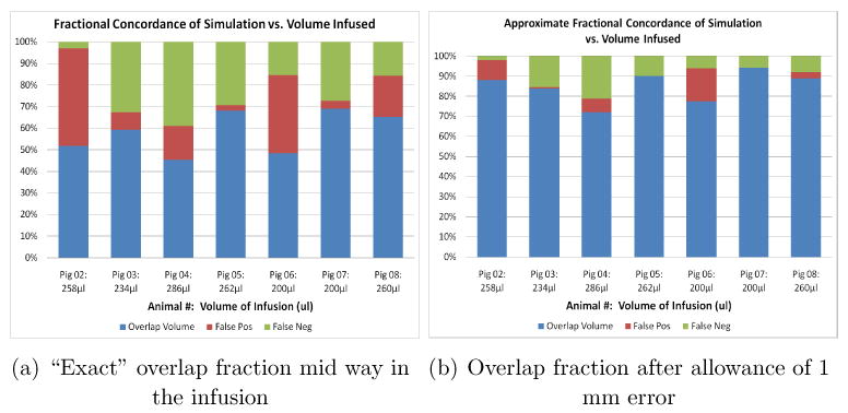
Two figures of merit (FOM) for comparing predicted distributions of tracer with the measured, for all the animals used. The total infused volumes in each case are noted at the bottom of the bars, and corresponds to roughly half way through the infusion process. The left hand graph FOM computes the number of voxels that have been filled by the tracer above the threshold concentration (see text) according to both the prediction and the measurement, as a fraction of the number in union of both predicted and measured voxels reached. The right hand graph shows the same numbers but allowance is now made to declare overlap even if the voxels are separated by one voxel width. The color code is explained in the text.
Figure 2.

Concordances computed exactly as for the previous graph, but now at the end of the infusion. Both FOM's, the exact and the relaxed, are shown.
It may be asked if raising the threshold will substantially worsen the overlap percentage. That the agreement cannot improve is obvious, since we are moving towards a more stringent comparison. We shall address this question by examining what happens in the two extreme cases, as measured by the above FOM, in the subsection below. To examine the goodness of fit of the the actual distributions, the correlation or root mean square deviation between the simulated and measured distributions is the usual measure used. We expect larger errors here, since this depends on a 1–1 correspondence of values, with noisy values in the margins of the infusion contributing significantly. We emphasize that there is a more important reason why this is less significant. After all, in short infusions, where there is little loss of tracer through the capillaries, and ignoring the diffusion in the outer margins, the concentration in the tissue is essentially a reflection of the interstitial volume fraction. In fact, the idealized picture of CED that is often presented describes the infusate as having a flat profile of concentration, meaning that the interstitial concentration is that in the infusate. Thus, if the volumes of distribution have been estimated well, errors in concentration estimation are essentially errors in interstitial expansion estimation. In other words, if we could compare the interstitial concentrations (which cannot be measured by MR imaging) then these would be much better (assuming the above FOM has come out well). We display the errors in our prediction of the tissue concentration, since that's what we can measure, in Figure (3), where the displayed error RMSE for each pig is defined by
Figure 3.

The RMS error in the predictions for all the animals, computed as specified in the text. The infused concentration is 2.5 mM/L for comparison.
| (15) |
Most of the errors are right around 10% of the infused concentration. We caution that there are errors in the measured valued as well. We have found that in many places the match is very good, and that the places where the match is not particularly so do contribute substantially to the error. We feel that the main value of measuring the concentrations is to understand the changes in interstitial volumes, which do greatly affect the distribution — see also the Conclusions — but which do not directly address the clinical issue of getting the appropriate dose to the region.
3.2.2.2. Spatial distribution profiles
We now examine the spatial distributions in the extreme cases mentioned. First, just for a reference to indicate the quality of our images, we show some coronal slices of the MRI for Pig 7. The quality of imaging is comparable for all animals, so it is sufficient to show it for one. In Figures 4 (a), (b), and (c) we show, respectively, a T1 weighted (SPGR with a 35° flip angle) image, the trace of the diffusion tensor and the fractional anisotropy map, all prior to the infusion. However, the catheter location can be seen in Figure 4 (a). Finally, in (d), we show the T1 weighted image obtained by the same pulse sequence as for (a), but after 105 minutes of infusion, with 440 μ L of fluid infused. After this time point, the Gd begins to leak out the top of the brain, and the infusion was discontinued.
Figure 4.

Some MR imaging on Pig 7 showing catheter placement (extreme left), sample DTI images to gauge the quality of the acquisition (middle two), and (rightmost) the T1-weighted image at the end of the infusion showing the enhancement due to the tracer.
The best case
Pig 7 was the “best case” behavior, as noted. The measured and simulated concentrations are shown in Figure 5, along with the SPGR image of Figure 4(a) in the background. Although all data is obtained in three dimensions, only plane sections are shown here. The color maps range from 2.5% to 50% of the infused concentration (2.5 mM / L). Figure 4(d) displays the overlap volumes: the image displays red as the volume (or, rather, area) of overlap, the measured distribution outside the overlap volume is green (false negative), and blue as the simulated distribution outside the overlap (false positive). We remark, in passing, that a comparison of 4(d) and of Figure 5(a) shows how difficult it is to read any nuances related to the profile of the spatial concentration from a contrast enhanced image. Conventional “volume of distribution” measures are of course based simply on the contrast enhanced image at a single flip angle. Other canonical sections, e.g., the sagittal show similar behavior so we have omitted these displays.
Figure 5.

Sample measured and predicted distributions in an coronal slice of Pig 7 at the end (105 minutes, 865 μL infused): measured and predicted distributions are color coded. The overlap volumes on the extreme right are colored as described in the text.
The worst case
There is of course more to discuss for the case where the fit was worst, namely Pig 4 shown in Figures 6 and 7. The data shown were taken at 96 minutes of infusion, and we show both coronal and sagittal views in this case. The color codes for the distribution volumes in the two left images are the same as for Pig 7, and so is the color code for the concentrations obtained by the simulation in the two rightmost images. The background in these images are the higher flip angle T1 weighted images taken at that time. The main discrepancies between the simulated vs measured are (i) that the Gd started leaking through the CSF along ventricles and subarachnoid from early in the infusion: as mentioned currently the simulation does not track leaked infusate; (ii) the simulation had longer backflow, and thus more distribution toward the superior side. This too may have arisen from the CSF. The catheter is at the edge of, or into, the edge of the ventricle. The actual backflow stops there, but the simulation goes back beyond the ventricle. The sagittal view is helpful to visualize the loss along CSF. (The quality of the DTI can be inferred from those shown for the Pig 7 slices and so we do not display these.)
Figure 6.

Sample measured and predicted distributions in an coronal slice of Pig 4 after 691 μL of infusion following the same pattern and color coding as the previous figure for Pig 7.
Figure 7.

Sample measured and predicted distributions in a sagittal slice of Pig 4 at the same time as for the displayed coronal slice of the previous figure.
It seems clear that two major sources of discrepancy between the computed and measured concentrations are (i) mis-estimation of interstitial volume changes, and (ii) disregarding losses into CSF spaces. The total Gd measurements demonstrated that a significant amount of the tracer was lost, increasing with the infusion time. There are two major paths for this loss. We have assumed the loss through the capillaries to be uniform across the tissue, and indeed across the animals. In addition, there is loss directly into the CSF spaces, both ventricles and brain surfaces, which will vary according to the infusion and the individual. Loss into CSF tends to disperse and dilute rapidly, making it difficult to track in the MR imaging. In the simulation model, CSF is treated as a sink for molecules entering, and are thus lost from the simulation, and not counted. There is thus a tendency to larger total Gd in the measured value, where some of the tracer in the CSF is measurable. These discrepancies then are greater in animals such as Pig 4 where these losses are particularly acute. We will be modifying the image analysis so that we do not count the measured Gd that has entered into the CSF. (This depends on our CSF segmentation, mentioned in Section 2.4.) As mentioned the overlap figures of merit show relatively good matches. We now examine raising the threshold used to examine the overlap fractions. Table 3 shows the result fo the two exemplars. As we see Pig 7 shows “graceful” degradation with raising the threshold. Pig 4 at mid-infusion also shows a modest change when the threshold is changed. However, the final concordances are significantly worse at the higher threshold, offering evidence again for the effect of the CSF losses. In all cases, the spatial profiles produced by the simulations tend to be smoother, rounder, and less sharply defined than those measured as just discussed. This is not surprising, given the limited resolution of the diffusion tensor imaging upon which the simulations are based, and our smooth estimation of the interstitial volume changes. We are currently working on these two limitations, as discussed briefly in the Conclusions.
Table 3.
Concordances with varying thresholds. See text for explanation.
| Exact @ 10% | Exact @2.5% | Relaxed@10% | Relaxed @2.5% | ||
|---|---|---|---|---|---|
| Pig 4 | Mid-term | 36.5% | 45% | 66% | 69% |
| Final | 30% | 49% | 59% | 75% | |
| Pig 7 | Mid-term | 63% | 69% | 93% | 93% |
| Final | 64% | 74% | 89% | 95% |
Finally, we should mention that there is variation in the distributions even though the placement of the catheter was within a mm or two of the same anatomical target in all the animals. For example, in Figure 8 we display coronal sections containing the line of the catheter for two pigs, at roughly corresponding points in the infusion, as the caption indicates. Even with the smaller amount infused, the shape of the distributions is different. These variations occur throughout the infusions examined. It is also interesting to note is the discrepancy in Figure 8 between the measured (c) and predicted (d) distributions for Pig 8. There seems to be a “neck” in the observed distribution, where the concentration of the tracer was too low to be displayed. It is possible that this is an effect of our model assumption which expands the interstitial spaces monotonically with the fractional anisotropy of the DTI. The neck is just above, and contiguous with, a region where the white matter fibers are impinging upon the gray, and have high anisotropy (and so expand, according to our model, and accommodate tracer). However, the ultrastructure of their organization may be perhaps be such that these fibers are crossed and taut, and do not allow much fluid to accumulate, so that the tracer in fact traverses this to fill the region above. This explanation is frankly speculative and awaits further work to be tested. Yet another mechanism of fluid distribution that we have not accounted for is perivascular flow. It is well known that major blood vessels, particularly arteries, seem to delineate high conductivity pathways within the interstitium for pressure–driven fluid flow [21]. The “hook” in Figure 8(a) on the upper left of the image may be an example of this. Currently, we are also imaging the blood vessels with non-invasive MR angiography, so we can remedy this omission in future studies in a way that can be applicable to humans.
3.3. Determinants of flow
The infusions reported upon here, as is customary in clinical infusions, were performed at specified flow rates. Thus at the end of a given time period, the volume of water we have infused will occupy the same volume in the interstitium (since water may be considered incompressible for our purposes). Thus, the principal determinants of the distribution of any marker of fluid are the backflow and the interstitial expansion, along with their interplay. In other words, the scale that sets the hydraulic conductivity is not particularly relevant in determining the distribution. It is true that changing the scale would result in a change of the pressure, but the latter simply enforces the constraint of the compressibility equation and does not determine the distribution. The expansion and the backflow are in intimate interplay. In the white matter infusions we performed, the interstitial expansion is considerable, and the initial front from which the fluid expands into tissue is set by the length of backflow which is affected by this expansion. One observation we noted is that the interstitial expansion based on observation of changes of T2 signal in white matter during infusion in human patients led us to a higher number for the maximum fraction of interstitial space (0.6), in comparison with the one we used to get the best fit for the porcine models (0.45). We arrived at this by varying the maximum value and observing the resulting distributions. We hesitate to ascribe a definite reason for this. It is known that the number density of cells overall in the cortex is lower in humans than in other higher mammals ([5], Table 232), while the fraction of these that are glial cells is considerably higher in the human than in the pig (∼ 1.4 : 1 according to Table 267 of the reference). Perhaps the more compact regions of porcine white matter may not allow as great an expansion at the typical rates of infusion.
The values quoted for the capillary hydraulic permeability are low enough not to matter. More precisely, the characteristic decay length , where K is a characteristic tissue hydraulic conductivity, is about 7 cm, by which time the 1/r behavior of an incompressible fluid has already dropped the pressure by more than the factor of e from the exponential dependence. So, varying the capillary permeabilities in a range within these small values will not affect the results. Finally, the degradation rate of the molecule of course can very significantly affect its distribution. That is why small molecules that easily penetrate even an intact blood brain barrier will not spread far in a CED infusion. However, our principal conclusion is that getting the backflow and the expanded, infusion-induced interstitial volume fraction is the important factor in describing the spread of the fluid which carries the drug or marker molecule. The distribution of the molecule itself can depend on its degradation rate and perhaps other factors particularly as its size approaches that of the interstitial widths (such as for viruses). Other conduits for flow such as the perivascular spaces also remain to be predicted.
3.4. Comparison with prior work
The key innovations in comparison to other simulations and models have already been discussed in Section 2.3.1: the backflow and the expansion are two of our contributions to the basic modeling in this field. Further, our approach was, as far as we know, the first individual-specific approach proposed and implemented. (The need for this is discussed in the last paragraph of this section.) This means in particular, that simulations should not be adjusted according to the individuals within a species or group, but that any variability be accounted for from data actually obtained from that individual. Previous computational models are in roughly two categories. One consists of entirely model–based calculations. What we mean is that these are computational results used to illustrate phenomena, but not compared directly with an experimental test. The excellent, first three–dimensional, computation of [51] is an example of this kind. There a model is used to suggest delivery routes for a drug (also a goal of our simulation) but the predicted quantitative data is not subjected to any experimental test. Rather, the parameters in the model are varied to construct “what if” scenarios. Certainly, this is a very valuable use of models, and Rakesh Jain and his co-workers have been investigating tumors, and drug delivery for tumors, for over two decades. Our simulations of course are also used this way [37], but then are similar to others in this category of modeling, apart from the novelties mentioned in the first sentence above. We include in this category the computations where either the parameter values used throughout are obtained from a judicious selection of the literature, or fitted to one particular dataset, and so of course, are not individual–specific. This approach also has been used extremely widely, e.g., [40], [39], and usually the comparison with data has been purely qualitative, as in examining the rough shape of an infusion. Our work, as far as we are aware, is the first quantitative examination of a computational model compared with a series of infusions.
The second category of computations is where a serious attempt is made to be individual–specific. There are essentially two ways in which such a simulation may be performed. One is the way we have approached it. The other is an atlas–based approach where statistics is collected over a number of infusions and a segmented brain is endowed with appropriate cytoarchitecture–specific parameters. One may call this essentially a system identification method of constructing a model. In fact, we included such an approach in our first description of simulations for planning drug discovery [34] and other people have also taken up such methods [22]. There are two problems with this approach. One is its very generality: the number of parameters needed to fit the data can be very large depending on how finely the brain (or other cytoarchitecture) is segmented, and how finely the interstitial expansion as a function of the location of the pressure source and fluid content is described. In fact, despite the many proposals, we are unaware of any studies that have even displayed the results and compared them with several infusions as we have. Another is that such models can and do miss the physics concerned. For example, endowing white matter with a high conductivity along the fiber tracks, will, it is true, result in more fluid flowing in those directions. But, as we have pointed out, this contradicts experimental results that show that edematous white matter in fact is hardly more anisotropic than gray: it is the expansion of the fluid–filled interstitium that results in the greater flow. It is important that a model not only fit data, but also that it is consistent with the physics of the infusion process, including expansion and backflow. However, an atlas–based approach, when the anatomy is warped well to fit the atlas, can indeed be another approach to an individual–specific model.
Finally, we mention that individual–specificity is a need whenever there is significant anatomic and physiological variation in the determinants of flow. (We of course pre-suppose that a minimal dose of therapeutic is desired within a designated target region, and constraints imposed on the efflux outside of this region.) Diseased tissue states where the extent and the physiological correlates of the disease are very variable are candidates for testing the utility of planning the infusions. Intraparenchymal therapeutic infusions for brain cancer [38], prostatic disease, and other solid tissue tumors are examples. In such cases, a physician cannot assess placement and flow rates for catheters by simply looking at an MR image, or even by having the computer plan according to a purely geometric approach where the catheter is placed sufficiently far from sulci and so on [37]. We hope to compare our simulations in such a case with a more generic model which takes into account only white and gray matter, say, to directly assess the importance of the specificity of our approach.
4. Conclusions
Our approach to an individual–specific prediction of infusions in intact brains is, we believe, very encouraging as the results above show, but faces some significant challenges. The first is that, key to the use of cross–property relations allowing us to infer a hydraulic conductivity from a diffusion tensor for example, is the ability to extract a purely extracellular diffusivity. This is not feasible as far as we can see under currently available clinical and non-invasive conditions on individual brains as discussed. The second challenge is that expansion of the interstitial spaces under the influence of both positive pressure and fluid content increase during infusion must be estimated, along with its consequences for the hydraulic conductivity — which rises very steeply with fluid content — and other parameters. Our scheme clearly depends on neither, being simply a gross cytoarchitectural estimate. As mentioned, this may not be too bad for the major white matter tracts, but will be inadequate for gray matter responses to fluid infusons. We are currently working with improved models for these nonlinear poroelastic effects that are also implementable in easily available hardware.
There is a large number of other improvements that may be made to the model as well as to the computation. Chief amongst these are the direct simulation of the fluid velocity field, incorporation of blood vessel conduits for flow (the perivascular spaces), improvement of the boundary conditions at the CSF spaces as mentioned in the text, and (computationally) exploiting massive parallelism from the graphics processors currently available. We are working on these improvements as well, which are more straightforward and offer fewer challenges than the two key issues mentioned above. We expect to report on all these in the future.
Acknowledgments
The research described in this paper was supported in part by grant number R44-NS043105-03 of the National Institutes of Health of the U. S. A. The experiments were conducted by Drs. Zhijian Chen, Dr. Panos Fatouros, and others at the Virginia Commonwealth University. These experimental results have been published separately [6]. The research was also supported by BrainLAB AG which has a direct commercial interest in the software so developed. We acknowledge very helpful comments from Dr. Inmaculada Rodriguez Ponce of BrainLAB AG. We are also grateful to two anonymous referees whose comments and suggestions, in succession, significantly altered and improved the presentation.
References
- 1.Abbott N Joan. Evidence for bulk flow of brain interstitial fluid: significance for physiology and pathology. Neurochemistry International. 2004;45:545–552. doi: 10.1016/j.neuint.2003.11.006. [DOI] [PubMed] [Google Scholar]
- 2.Alexander Daniel C, Hubbard Penny L, Hall Matt G, Moore Elizabeth A, Ptito Maurice, Parker Geoff J M, Dyrby Tim B. Orientationally invariant indices of axon diameter and density from diffusion MRI. Neuroimage. 2010;52:1374–1389. doi: 10.1016/j.neuroimage.2010.05.043. [DOI] [PubMed] [Google Scholar]
- 3.Basser Peter J, Jones Derek K. Diffusion tensor MRI: theory, experimental design and data analysis – a technical review. NMR in Biomedicine. 2002;15:456–467. doi: 10.1002/nbm.783. [DOI] [PubMed] [Google Scholar]
- 4.Bear J. Dynamics of Fluids in Porous Media. Dover. 1988 [Google Scholar]
- 5.Blinkov Samuil M, Glezer Il'ya I. The Human Brain In Figures And Tables. In: Haigh Basil., translator. Basic Books Incorporated. Plenum Press; 1981. [Google Scholar]
- 6.Brady Martin, Raghavan Raghu, Chen Zhi jian, Broaddus William C. Quantifying fluid infusions and tissue expansion in brain. IEEE Transactions on Biomedical Engineering. 2011 doi: 10.1109/TBME.2011.2128869. in press. [DOI] [PubMed] [Google Scholar]
- 7.Bruch LW, Zaremba Eugene, Cole Milton W. Physical Adsorption: Forces and Phenomena. 1997 [Google Scholar]
- 8.Chen Kevin C, Nicholson Charles. Changes in brain cell shape create residual extracellular space volume and explain tortuosity behavior during osmotic challenge. Proceedings of the National Academy of Sciences, USA. 2000;97:8306–8311. doi: 10.1073/pnas.150338197. [DOI] [PMC free article] [PubMed] [Google Scholar]
- 9.Chen MY, Lonser RR, Morrison PF, Governale LS, Oldfield EH. Variables affecting convection-enhanced delivery in the striatum: a systematic examination of rate of infusion, cannula size, infusate concentration, and tissue-cannula sealing time. Journal of Neurosurgery. 1999;90:315–320. doi: 10.3171/jns.1999.90.2.0315. [DOI] [PubMed] [Google Scholar]
- 10.Coussy Olivier. Poromechanics. John Wiley and sons. 2004 [Google Scholar]
- 11.Craciun Gheorge, Brown Anthony, Friedman Avner. A dynamical system model of neurofilament transport in axons. Journal of Theoretical Biology. 2005;237:316–322. doi: 10.1016/j.jtbi.2005.04.018. [DOI] [PMC free article] [PubMed] [Google Scholar]
- 12.Croteau D, Walbridge S, Morrison PF, Butman JA, Vormeyer AO, Johnson D, Oldfield EH, Lonser RR. Real time, in vivo imaging of convective distribution of a low molecular weight tracer. Journal of Neurosurgery. 2005;102:90–107. doi: 10.3171/jns.2005.102.1.0090. [DOI] [PubMed] [Google Scholar]
- 13.Deoni SCL, Peters TM, Rutt BK. Determination of optimal angles for variable nutation proton magnetic spin-lattice, T1, and spin-spin T2, relaxation times measurement. Magnetic Resonance in Medicine. 2004;51:194–199. doi: 10.1002/mrm.10661. [DOI] [PubMed] [Google Scholar]
- 14.Deoni SCL, Rutt BK, Peters TM. Rapid combined T1 and T2 mapping using gradient recalled acquisition in the steady-state. Magnetic Resonance in Medicine. 2003;49:515–526. doi: 10.1002/mrm.10407. [DOI] [PubMed] [Google Scholar]
- 15.Ding Dale, Kanaly Charles W, Brady Martin L, Mittermeyer Stephan, Raghavan Raghu, Sampson John H. Convection-enhanced delivery to the brain. Drug Delivery to the Central Nervous System. 2010:291–318. [Google Scholar]
- 16.Fan Xijun, Phan-Thien Nhan, Wu Ng Teng Yong Xuhong, Xu Diao. Microchannel flow of a macromolecular suspension. Physics of Fluids. 2003;15:11–21. [Google Scholar]
- 17.Freidlin Mark. Functional Integration and Partial Differential Equations. Princeton University Press; 1985. [Google Scholar]
- 18.Friedman Avner, Craciun Gheorge. A model of intracellular transport of particles in an axon. Journal of Mathematical Biology. 2005;51:217–246. doi: 10.1007/s00285-004-0285-3. [DOI] [PubMed] [Google Scholar]
- 19.Goh Yin Min Felicia, Kong Hwai Loong, Wang Chi Hwa. Simulation of the delivery of doxorubicin to hepatoma. Pharmaceutical Research. 2001;18:761–770. doi: 10.1023/a:1011076110317. [DOI] [PubMed] [Google Scholar]
- 20.Groothuis Dennis R, Ward Sherman, Schlageter Kurt E, Itskovich Andrea C, Schwerin Susan C, Allen Cathleen v, Dills Cynthia, Levy Robert M. Changes in blood-brain permeability associated with the insertion of brain cannulas and microdialysis probes. Brain Research. 1998;803:218–230. doi: 10.1016/s0006-8993(98)00572-1. [DOI] [PubMed] [Google Scholar]
- 21.Hadaczek Piotr, Yamashita Yoji, Mirek Hanna, Tamas Laszlo, Bohn Martha C, Noble Charles, Park John W, Bankiewicz Krystof. The “perivascular pump” driven by arterial pulsation is a powerful mechanism for distribution of therapeutic molecules within the brain. Molecular Therapy. 2006;14:69–78. doi: 10.1016/j.ymthe.2006.02.018. [DOI] [PMC free article] [PubMed] [Google Scholar]
- 22.Linninger AA, Somayaji MR, Zhang Libin, Hariharan MS, Penn RD. Rigorous mathematical modeling techniques for optimal delivery of macromolecules to the brain. IEEE Transactions on Biomedical Engineering. 2008;55:2303–2313. doi: 10.1109/TBME.2008.923920. [DOI] [PubMed] [Google Scholar]
- 23.Linninger Andreas A, Somayaji Mahadevabharath R, Mekarski Megan, Zhang Libin. Prediction of convection-enhanced delivery to the human brain. Journal of Theoretical Biology. 2008;250:125–138. doi: 10.1016/j.jtbi.2007.09.009. [DOI] [PubMed] [Google Scholar]
- 24.Lonser RR, Gogate N, Wood JD, Morrison PF, Oldfield EH. Direct convective delivery of macromolecules to the peripheral nerves. Journal of Neurosurgery. 1998;89:610–615. doi: 10.3171/jns.1998.89.4.0610. [DOI] [PubMed] [Google Scholar]
- 25.Lonser RR, Walbridge S, Garmestani K, Butman JA, Walters HA, Vortmeyer AO, Brechbiel MW, Morrison PF, Oldfield EH. Successful and safe perfusion of the primate brainstem with a macromolecule: in vivo magnetic resonance imaging of macromolecular distribution during infusion. Journal of Neurosurgery. 2002;97:905–913. doi: 10.3171/jns.2002.97.4.0905. [DOI] [PubMed] [Google Scholar]
- 26.Lonser RR, Weil RJ, Morrison PF, Governale LS, Oldfield EH. Direct convective delivery of macromolecules to the spinal cord. Journal of Neurosurgery. 1998;89:616–622. doi: 10.3171/jns.1998.89.4.0616. [DOI] [PubMed] [Google Scholar]
- 27.Morrison PF, Laske DW, Bobo H, Oldfield EH, Dedrick RL. High flow microinfusion: tissue penetration and pharmacodynamics. American Journal of Physiology: Regulatory, Integrative, and Comparative Physiology. 1994;266:R292–R305. doi: 10.1152/ajpregu.1994.266.1.R292. [DOI] [PubMed] [Google Scholar]
- 28.Morrison PF, Chen MY, Chadwick RS, Lonser RR, Oldfield EH. Focal delivery during direct infusion to brain : role of flow rate, catheter diameter, and tissue mechanics. American Journal of Physiology: Regulatory, Integrative, and Comparative Physiology. 1999;277:R1218–1229. doi: 10.1152/ajpregu.1999.277.4.R1218. [DOI] [PubMed] [Google Scholar]
- 29.Panagiotaki Eleftheria, Fonteijn Hubert, Siow Bernard, Hall Matt G, Price Anthony, Lythgoe Mark F, Alexander Daniel C. Two-compartment models of the diffusion MR signal in brain white matter. Proceedings of MICCAI. 2009;1:329–336. doi: 10.1007/978-3-642-04268-3_41. [DOI] [PubMed] [Google Scholar]
- 30.Pardridge William M. The blood-brain barrier: bottleneck in brain drug development. NeuroRx: the Journal of the American Society for Experimental Neurotherapeutics. 2005;2:3–14. doi: 10.1602/neurorx.2.1.3. [DOI] [PMC free article] [PubMed] [Google Scholar]
- 31.Pluen Alain, Netti Paolo A, Jain Rakesh, Berk David A. Diffusion of macromolecules in agarose gels: comparison of linear and globular configurations. Biophysical Journal. 1999;77:542–552. doi: 10.1016/S0006-3495(99)76911-0. [DOI] [PMC free article] [PubMed] [Google Scholar]
- 32.Press William H, Flannery Brian P, Teukolsky Saul A, Vetterling William T. Numerical Recipes in C: the Art of Scientific Computing. Cambridge University Press; 1992. [Google Scholar]
- 33.Raghavan Raghu, Mikaelian Samuel, Brady Martin, Chen Zhi Jian. Fluid infusions from catheters into elastic tissue I: azimuthally symmetric backflow in homogeneous media. Physics in Medicine and Biology. 2010;55:281–304. doi: 10.1088/0031-9155/55/1/017. [DOI] [PubMed] [Google Scholar]
- 34.Raghavan Raghu, Poston Timothy, Viswanathan Raju. A method and apparatus for targeting material delivery to tissue. United States Patent 6,549,803. 2003 April;(15)
- 35.Reisfeld B, Kalyanasundaram S, Leong K. A mathematical model of polymeric controlled drug release and transport in the brain. Journal of Controlled Release. 1995;36:199–207. [Google Scholar]
- 36.Reulen Hans J, Graham Robert, Spatz Maria, Katzo Igor. Role of pressure gradients and bulk flow in dynamics of vasogenic brain edema. Journal of Neurosurgery. 1977;46:24–35. doi: 10.3171/jns.1977.46.1.0024. [DOI] [PubMed] [Google Scholar]
- 37.Sampson JH, Archer GE, Pedain C, Wembacher-Schroder E, Westphal M, Kunwar S, Vogelbaum MA, Coan A, Herndon JE, Raghavan R, Brady ML, Reardon DA, Friedman AH, Friedman HS, Rodriguez-Ponce I, Chang S, Mittermeyer S, Croteau D, Puri R. Poor drug distribution as a possible explanation for the results of the PRECISE trial. Journal of Neurosurgery. 2010;113:301–309. doi: 10.3171/2009.11.JNS091052. [DOI] [PubMed] [Google Scholar]
- 38.Sampson John H, Raghavan Raghu, Brady Martin L, Provenzale James M, Herndon James E, Croteau David, Friedman Allan H, Reardon David A, Edward Coleman R, Wong Terence, Bigner Darell D, Pastan Ira, Rodriguez-Ponce Maria Inmaculada, Tanner Philipp, Puri Raj, Pedain Christoph. Clinical Utility of a Patient-specific Algorithm for Simulating Intracerebral Drug Infusions. Neuro-Oncology. 2007;9:343–353. doi: 10.1215/15228517-2007-007. [DOI] [PMC free article] [PubMed] [Google Scholar]
- 39.Sartinoranont M, Banerjee A, Lonser RR, Morrison PF. Direct interstitial infusion of NK1-targeted neurotoxin into the spinal cord: a computational model. American Journal of Physiology: Regulatory, Integrative, and Comparative Physiology. 2003;285:R243–R254. doi: 10.1152/ajpregu.00472.2002. [DOI] [PubMed] [Google Scholar]
- 40.A computational model of direct interstitial infusion of macromolecules into the spinal cord. Annals of Biomedical engineering. 2003;31:448–461. doi: 10.1114/1.1558032. [DOI] [PubMed] [Google Scholar]
- 41.Schnitzer Mark J. Theory of continuum random walks and application to chemotaxis. Physical Review E. 1993;48:2553–2568. doi: 10.1103/physreve.48.2553. [DOI] [PubMed] [Google Scholar]
- 42.Sivaloganathan S, Stastna M, Tenti G, Drake JM. Biomechanics of the brain: A theoretical and numerical study of Biot's equations of consolidation theory with deformation-dependent permeability. International Journal of Non-linear Mechanics. 2005;40:1149–1159. [Google Scholar]
- 43.Smith Joshua H, Humphrey Joseph AC. Interstitial transport and transvascular fluid exchange during infusion into brain and brain tissue. Journal of Microvascular Research. 2006;2:871–882. doi: 10.1016/j.mvr.2006.07.001. [DOI] [PubMed] [Google Scholar]
- 44.Sykova E, Svoboda J, Polak J, Chvatal A. Extracellular volume fraction and diffusion characteristics during progressive ischemia and terminal anoxia in the spinal cord of the rat. Journal of Cerebral Blood Flow and Metabolism. 1994;14:301–311. doi: 10.1038/jcbfm.1994.37. [DOI] [PubMed] [Google Scholar]
- 45.Sykova Eva, Mazel Tomas, Vargova Lydia, Vorisek Ivan, Prokopova-Kubinova Sarka. Extracellular space diffusion and pathological states. Progress in Brain Research. 2000;125:155–178. doi: 10.1016/S0079-6123(00)25008-5. [DOI] [PubMed] [Google Scholar]
- 46.Tenti G, Sivaloganathan S, Drake JM. The synchrony of arterial and CSF pulsations is not due to resonance. Pediatric Neurosurgery. 2002;37:221–222. doi: 10.1159/000065400. [DOI] [PubMed] [Google Scholar]
- 47.Thelwall P, Grant Samuel C, Stanisz Greg J, Blackband Stephen J. Human erythrocyte ghosts: exploring the origins of multiexponential water diffusion in a model biological tissue with magnetic resonance. Magnetic Resonance in Medicine. 2002;48:649–657. doi: 10.1002/mrm.10270. [DOI] [PubMed] [Google Scholar]
- 48.Thorne Robert G, Nicholson Charles. In vivo diffusion analysis with quantum dots and dextrans predicts the width of brain extracellular space. Proceedings of the National Academy of Sciences. 2006;103:5567–5572. doi: 10.1073/pnas.0509425103. [DOI] [PMC free article] [PubMed] [Google Scholar]
- 49.Torquato S. Random Heterogeneous Materials. Springer; 2000. [Google Scholar]
- 50.Tuch DS, Wedeen VJ, Dale AM, George JS, Belliveau JW. Conductivity tensor mapping of the human brain using diffusion tensor MRI. Proceedings of the National Academy of Sciences. 2001;98:11697–11701. doi: 10.1073/pnas.171473898. [DOI] [PMC free article] [PubMed] [Google Scholar]
- 51.Wang Chi Hwa, Li Jian. Three-dimensional simulation of IgG delivery to tumors. Chemical Engineering Science. 1998;53:3579–3600. [Google Scholar]
- 52.Wang Herb. Linear Theory of Poroelasticity. Princeton University Press; 2000. [Google Scholar]
- 53.Zhang Xiao Yu, Luck Jason, Dewhirst Mark W, Yuan Fan. Interstitial hydraulic conductivity in a fibrosarcoma. American Journal of Physiology Heart Circulation Physiology. 2000;279:H2726–H2734. doi: 10.1152/ajpheart.2000.279.6.H2726. [DOI] [PubMed] [Google Scholar]