Multi-scale Inference of Interaction Rules in Animal Groups Using Bayesian Model Selection

Abstract

Inference of interaction rules of animals moving in groups usually relies on an analysis of large scale system behaviour. Models are tuned through repeated simulation until they match the observed behaviour. More recent work has used the fine scale motions of animals to validate and fit the rules of interaction of animals in groups. Here, we use a Bayesian methodology to compare a variety of models to the collective motion of glass prawns (Paratya australiensis). We show that these exhibit a stereotypical ‘phase transition’, whereby an increase in density leads to the onset of collective motion in one direction. We fit models to this data, which range from: a mean-field model where all prawns interact globally; to a spatial Markovian model where prawns are self-propelled particles influenced only by the current positions and directions of their neighbours; up to non-Markovian models where prawns have ‘memory’ of previous interactions, integrating their experiences over time when deciding to change behaviour. We show that the mean-field model fits the large scale behaviour of the system, but does not capture fine scale rules of interaction, which are primarily mediated by physical contact. Conversely, the Markovian self-propelled particle model captures the fine scale rules of interaction but fails to reproduce global dynamics. The most sophisticated model, the non-Markovian model, provides a good match to the data at both the fine scale and in terms of reproducing global dynamics. We conclude that prawns' movements are influenced by not just the current direction of nearby conspecifics, but also those encountered in the recent past. Given the simplicity of prawns as a study system our research suggests that self-propelled particle models of collective motion should, if they are to be realistic at multiple biological scales, include memory of previous interactions and other non-Markovian effects.

Author Summary

The collective movement of animals in a group is an impressive phenomenon whereby large scale spatio-temporal patterns emerge from simple interactions between individuals. Theoretically, much of our understanding of animal group motion comes from models inspired by statistical physics. In these models, animals are treated as moving (self-propelled) particles that interact with each other according to simple rules. Recently, researchers have shown greater interest in using experimental data to verify which rules are actually implemented by a particular animal species. In our study, we present a rigorous selection between alternative models inspired by the literature for a system of glass prawns. We find that the classic theoretical models can accurately capture either the fine-scale behaviour or the large-scale collective patterns of movement of the prawns. However, none are able to reproduce both levels of description at the same time. To resolve this conflict we introduce a new class of models wherein prawns ‘remember’, their previous interactions, integrating their experiences over time when deciding to change behaviour. These outperform the traditional models in predicting when individual prawns will change their direction of motion and restore consistency between the fine-scale rules of interaction and the global behaviour of the group.

Introduction

The most striking features of the collective motion of animal groups are the large-scale patterns produced by flocks, schools and other groups. These patterns can extend over scales that exceed the interaction ranges of the individuals within the group [1]–[4]. For most flocking animals, the rules dictating the interactions between individuals, which ultimately generate the behaviour of the whole group, are still not known in any detail. Many ‘self-propelled’ particle models have been proposed for collective motion, each based on a relatively simple set of interaction rules between individuals moving in one, two or three dimensions [2], [5]–[8]. Typically these models implement a simple form of behavioural convergence, such as aligning the focal individual's velocity in the average direction of its neighbours or attraction towards the position of those neighbours. Generally such rules are explicitly kept as simple as possible while remaining realistic, with the aim of explaining as much as possible of collective motion from the simplest constituent parts.

Each of the models in the literature is capable of reproducing key aspects of the large-scale behaviour of one or more biological systems of interest. Together these models help explain what aspects of inter-individual interactions are most important for creating emergent patterns of coherent group motion. With this proliferation of putative interaction rules has come the recognition that some patterns of group behaviour are common to many models, and that different models can have large areas of overlapping behaviour depending on the choice of parameters [3]. Common patterns of collective behaviour are also observed empirically across a diverse range of animal and biological systems. For example, a form of phase transition from disorder to order has been described in species as diverse as fish [9], ants [10], locusts [11], down to cells [12] and bacteria [13]. In all these systems, as density of these species is increased there is a sudden transition from random disordered motion to ordered motion with the group collectively moving in the same direction. These studies indicate that a great deal can be understood about collective behaviour without reduction to the precise rules of interaction.

In many contexts however the rules of interaction are of more interest than the group behaviour they lead to. For example, when comparing the evolution of social behavior across different species, it is important to know if the same rules evolved independently in multiple instances, or whether each species evolved a different solution to the problem of behaving coherently as a group [1]. Recently researchers in the field have become interested in using tracking data from real systems on the fine scale to infer what precise rules of motion each individual uses and how they interact with the other individuals in the group [14]–[19]. This is an important trend in the field of collective motion as we move from a theoretical basis, centred around simulation studies, to a more data-driven approach.

The most frequent approach to inferring these rules has been to find correlations between important measurable aspects of the behaviour of a focal individual and its neighbours. For example, Ballerini et al. [14] looked at how a focal individual's neighbours were distributed in space relative to the position of the focal individual itself in a group of starlings. Significant anisotropy in the position of the -th nearest neighbour, averaged over all individuals, was regarded as evidence for an interaction between each bird and that neighbour. More recently Katz et al. [18] and Herbert-Read et al. [19] investigated how the change in velocity of each individual in groups of fish was correlated to the positions and velocities of the neighbouring fish surrounding the focal individual. This provides evidence not only for the existence of an interaction between neighbours but also estimates the rules that determine that interaction.

In these studies the rules of interaction are presented non-parametrically and cannot be immediately translated into a specific self-propelled particle model. Nor are these models validated in terms of the global schooling patterns produced by the fish. An alternative model-based approach that does fit self-propelled particle and similar models to data is proposed by Eriksson et al. [16] and Mann [17]. Under this approach, the recorded fine-scale movements of individuals are used to fit the parameters of, and select between, these models in terms of relative likelihood or quality-of-fit. This approach has the advantage of providing a parametric ‘best-fit’ model and can provide a quantitative estimate the relative probability of alternative hypotheses regarding interactions.

What all previous empirical studies have lacked is a simultaneous verification of a model at both the individual and collective level. Either fine scale individual-level behaviour is observed without explicit fitting of a model [18], [19] or global properties, such as direction switches [11], [20], speed distributions [21], [22] or group decision outcome [23] have been compared between model and data. Verification at multiple scales is the necessary next step now that inference based on fine-scale data is becoming the norm. Just as simulations of large-scale phenomena can appear consistent with observations of group behaviour without closely matching the local rules of interaction, so can fine-scale inferred rules be inconsistent with large-scale phenomena if these rules of inferred from too limited a set of possible models or from correlations between the wrong behavioural measurements. The closest that any study so far has come to finding consistency between scales has been Lukeman et al. [15]. In their study the local spatial distribution of neighbouring individuals in a group of scoter ducks was used to propose parametric rules of interaction, with some parameters measured from the fine-scale observables, but with others left free to be fitted using large-scale data. We suggest that if group behaviour emerges from individual interactions, then the form of these interactions should be inferable solely from fine-scale data without additional fitting at the large-scale. An inability to replicate the group behaviour using a selected model demonstrates that the model space has been insufficiently explored. When faced with alternative hypothesised interaction rules, model-based parametric inference provides the best means of quantitatively selecting between them.

In this paper we study the collective motion of small groups of the glass prawn, Paratya australiensis. Paratya australiensis is an atyid prawn which is widepsread throughout Australia [24]. Although typically found in large feeding aggregations, it does not appear to form social aggregations and has not been reported to exhibit collective behaviour patterns in the wild. We conduct a standard ‘phase transition’ experiment [9], [11], [12], studying how density affects collective alignment of the prawns. We complement this approach by using Bayesian inference to perform model selection based on empirical data at a detailed individual level. We select between models by calculating the probability of the fine scale motions using a Bayesian framework specifically to allow fair comparison between competing models of varying complexity. Comparison of the marginal likelihood, the probability of the data conditioned on the model, integrating over the uncertain parameter values, is a well developed and robust means of model selection that forms the core of the Bayesian methodology [25]–[28]. In adopting this approach, we reject the dichotomy of model inference based on either fine scale behaviour of the individuals or the motion of the group. Instead we use reproduction of the large scale dynamics through simulation as a necessary but not sufficient condition of the correct model.

Results

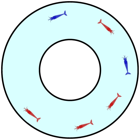
We study the positions and directions of co-moving prawns in a confined annular arena (See Methods and Materials and Figure 1). We tracked, using semi-automated software, the position of each prawn through the duration of the experiments. We pre-processed those raw tracking data by using a Hidden Markov Model to classify the movements of each prawn into a binary sequence of clockwise (CW) and anti-clockwise orientation (see Methods and Materials).

Figure 1. Schematic of the experimental setup.

Prawns moving within an annulus of 200 mm external diameter and 70 mm internal diameter. Red coloured prawns indicate a clockwise orientation, blue prawns a counter-clockwise orientation. In this instance the total number of prawns , number of clockwise-moving oriented prawns , the polarisation , and the excess polarisation .

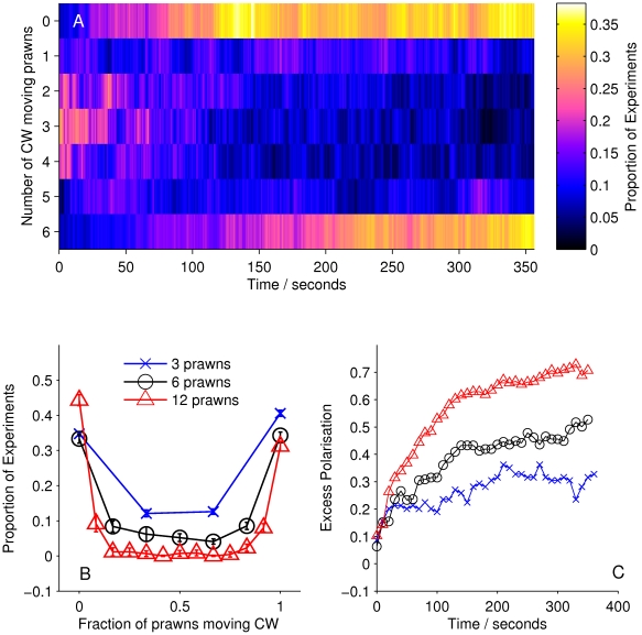
We then calculated the number of prawns travelling CW or anti-CW at each time step of each experiment involving three, six or twelve prawns. From this we calculated the average number of CW and anti-CW prawns at a given time across experiments. Figure 2A shows how the number of CW prawns, , changes over time, taken as a distribution over all trials with six prawns. There is a transition from an initially random configuration, with most trials having , to a final configuration where most experiments have either or . The final stable distribution is further shown in Figure 2B along with the final distribution for three and twelve prawn experiments. Steady state polarisation increases as a function of prawn number. The polarisation, can be defined as

(1)

The expected polarisation in randomly oriented groups varies with the number of individuals in the arena, being larger for smaller groups and obeying a binomial distribution. We adjust the measured polarisation by this expectation, , to obtain the excess polarisation, . Figure 2C shows this measure of polarisation over time for experiments with three, six and twelve prawns, confirming that the excess polarisation increases over time and is greater for larger groups.

Figure 2. Large-scale behaviour of the experimental system.

(A) The proportion of six-prawn experiments () with a given number of CW moving prawns over time. For each point in time we calculated the distribution over all trials of the number of CW prawns. This distribution is then plotted as a heat map. (B) The final distribution of experiments with number of CW moving prawns, for three-, six- and twelve-prawn experiments ( respectively). Error bars represent the mean and standard deviation for each proportion as calculated from the final ten seconds of the experiments. (C) The average polarisation of experiments with three, six and twelve prawns over time, adjusted by the expected polarisation of randomly oriented prawns.

At a group level we see that prawns tend to align over time, producing a polarised stable state, which is higher for larger group sizes. We define the reproduction of these global patterns as the global consistency condition of our model. We insist that any realistic model for the prawns' interactions must reproduce this large-scale behaviour.

Model selection

Next we investigated a series of interaction models as to their ability to reproduce the fine scale interactions of the prawns. We predict the probability, , that a focal prawn will change its orientation, given one of a number of potential models. The direction changes are determined by the data from the six-prawn treatment. This treatment provides the best balance between the number of data points, density of direction changes, clear large scale behaviour and tracking accuracy.

Each model specifies the probability that a focal prawn will change its direction in the next time step conditioned on the relative positions and directions of the other individuals in the arena. We use a logistic mapping to ensure probabilities remain between zero and one, so each model uses the relevant variables to determine a latent ‘turning-intensity’, , such that,

(2)

where is a function of the relative positions and directions of the other prawns, both now and potentially in the recent past, and the model parameters.

The models are, in increasing degree of complexity, as follows. Firstly to consider models that do not include zones-of-interaction – non-spatial models. We establish a baseline with a Null model. This simply posits that direction changes occur at random, at the rate established from the single prawn data, and the prawns do not interact in any way that changes this direction-changing probability. Therefore is given simply by a baseline constant, , which is determined by the rate of direction changing in single prawns.

(3)

We also consider two models where the interaction is independent of absolute spatial separation. The Mean Field (MF) model includes interactions between all prawns regardless of position, such that their relative directions alter the probability of changing direction. Since the number of prawns in the experiment is fixed, the probability for a direction change is influenced by the number of individuals moving in the opposite direction (negative prawns), . Each negative prawn increases the turning intensity by an amount ,

(4)

A Topological (T) model restricts these interactions to a limited number of nearest-neighbours, , the individuals closest to the focal prawn. The turning intensity is now influenced by the number of negative prawns, within the set of nearest-neighbours.

(5)

Secondly we consider a class of Spatial models (S1–S4). These models closely resemble the classic one-dimensional self-propelled particle models from the literature [5]. The focal prawn interacts with neighbours within a spatial zone-of-interaction, . The number and directions of individuals within this interaction zone determine the probability of changing direction. A number of further variations are possible; interactions can be limited to prawns ahead of the focal prawn and/or to prawns travelling in the opposite direction to the focal prawn. We consider four variations, indicated in Table 1. The general form for this model is given by,

(6)

where and are the number of negative and positive (travelling in the same direction) prawns within the interaction zone, and and parameterise the influence of each individual on the turning intensity. Interactions can occur with negative prawns only, , or with both negative and positive oriented prawns, . The spatial interaction zone is either a symmetrical area centred on the focal prawn, of width radians around the ring (spatial symmetric models in Table 1), or is only directed radians ahead of the focal prawn (spatial forward models).

Table 1. Model comparison.

Model	Interaction zone		/rads					KL/bits	/bits	Consistent?
Null	None	−7.5	N/A	N/A	N/A	N/A	N/A	10.2	−944	No
MF	Global	−7.5	N/A	N/A	0.51	N/A	N/A	0.6	−863	Yes
T	K nearest-neighbours	−7.5	N/A	3.4	0.72	N/A	N/A	2.0	−864	No
S1	Spatial, symmetric	−7.5		N/A	1.42	N/A	N/A	1.3	−847	No
S2	Spatial, forward	−7.5		N/A	1.71	N/A	N/A	7.2	−834	No
S3	Spatial, symmetric	−7.5		N/A	1.80	−0.01	N/A	2.0	−856	No
S4	Spatial, forward	−7.5		N/A	1.74	0.20	N/A	2.3	−859	No
D1	Spatial, symmetric	−7.5		N/A	1.62	N/A	0.47	0.7	−827	Yes
D2	Spatial, forward	−7.5		N/A	1.50	N/A	0.46	1.5	−830	No
D3	Spatial, symmetric	−7.5		N/A	1.44	0.23	0.87	0.4	−828	Yes
D4	Spatial, forward	−7.5		N/A	1.44	0.37	0.82	0.8	−830	Yes

The interaction zone structure of each model, along with the (mean a posteri ) inferred values of model parameters, an indicator for the model's consistency with the observed large scale behaviour of the real system, The KL divergence between experimental and model results indicating large-scale goodness-of-fit and the log marginal likelihood () of the model calculated from the fine scale dynamics (as shown in Figure 3). N/A indicates that the model does not include the indicated parameter. The interaction zone indicates whether prawns interact with others in a spatial zone around themselves, which may be oriented either forwards or symmetrically around their centre, or with their nearest-neighbours or globally with all other individuals. Reported parameters are: , the baseline direction-change intensity; , the interaction radius for spatial models; , the number of interacting nearest-neighbours for topological models; and , the strength of interaction with negative and positive prawns respectively; and , the decay factor determining how long interaction effects persist.

Visual inspection of the movements of the prawns suggests that interactions often follow a particular pattern. Two prawns, travelling in the opposite directions, collide. After the prawns have passed each other one of the prawns may subsequently decide to change direction. Self-propelled particle and other models of collective motion do not capture this type interaction. Such interactions are non-Markovian, i.e. the change in direction is not just the result of the environment now, but of the past environment as well. We proposed a third class of models (D1–D4), simple non-Markovian extensions of the basic spatial models, where each prawn would ‘remember’ the other individuals it encountered, with those memories fading at an unknown rate after the interaction was complete. As such the prawn would integrate those interactions over time, building up experiences which would alter its chance of changing direction. Mathematically this means that the turning intensity is now auto-regressive, depending on its own value at the previous time step as well as the current positions and directions of the neighbouring individuals. We introduce a decay parameter, , which determines how quickly the turning intensity returns to normal after an interaction with a neighbour has occurred. The same variations of interaction are allowed as for the spatial models, giving a general form for the non-Markovian turning intensity as,

(7)

where now indicates the turning intensity at time , which depends on the value of the turning intensity at the previous time step, . The number of prawns still in the interaction zone from time is indicated by , while the number of new arrivals in the interaction zone is given by . Hence raised (or lowered) turning intensities persist over time, with a duration controlled by the value of . After the focal prawn changes direction the turning intensity is reset to the baseline, , at the next time step.

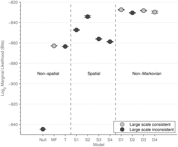
Table 1 specifies the interaction zone structure for each of eleven alternative models, grouped according to the description given above. For each model we calculate the marginal likelihood of the data, conditioned on the interaction model (see Methods and Materials). The marginal likelihood is the appropriate measure for performing model selection, especially between models of varying complexity. More complex models, by which we mean models with a larger number of free parameters, are penalised relative to simpler models when integrating over the parameter space, since less probability can be assigned to any particular parameter value a priori. The marginal likelihood indicates how likely a particular model is, rather than a model and an chosen optimal parameter value (see, for example, Mackay [29] Chapter 28 and other standard texts for discussions on this topic). The marginal likelihoods of each model are shown in Figure 3.

Figure 3. The marginal-likelihood of different models calculated from the fine scale dynamics.

Each marginal-likelihood is calculated by importance sampling. The figure shows the mean and standard error from 10 instances, each of 5000 samples. Grey markers indicate models that are consistent with the observed large scale behaviour of the system, black markers indicate those that are not. Consistency is determined by alignment of the prawns towards CW or anti-CW movement in simulations.

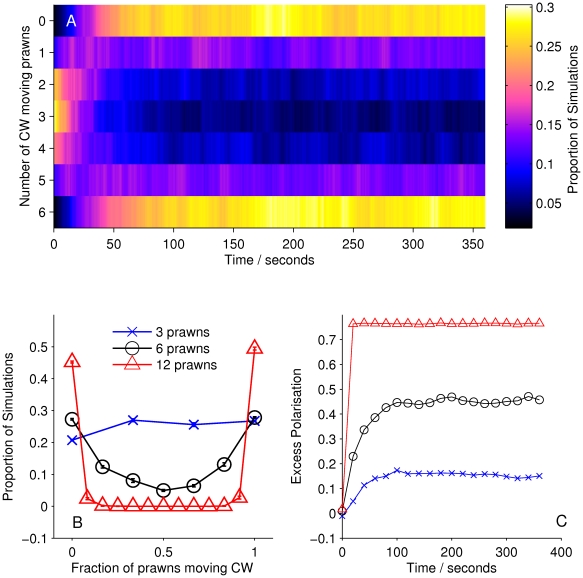
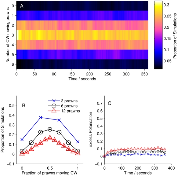
The Null model, in which prawns do not interact, performs significantly worse than the mean-field model. Figure 4 shows that the mean-field model fulfills our global consistency condition, reproducing an increase in polarization with time and prawn number. These results show that the prawns interactions involve matching their directions to that of others, producing alignment.

Figure 4. Simulation results for model MF.

(A) Proportion of six-prawn simulations () of mean-field model MF with a given number of prawns moving CW over time. (B) Final distribution of simulations by number of CW moving prawns for simulations with three, six and twelve prawns. Error bars represent the mean and standard deviation for each proportion as calculated from the final ten seconds of the simulations. (C) The average polarisation over time, adjusted by the expected polarisation of randomly oriented prawns, for simulations of three, six and twelve prawns. The KL divergence between the experimental and simulated results is 0.60 bits.

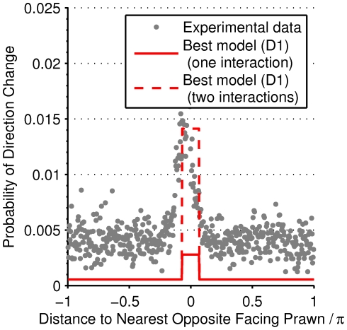
Are local spatial interactions important in reproducing observed direction changes? We note first that a topological interaction zone, where the focal prawn interacts with its nearest neighbours, has a marginal likelihood slightly lower than the mean field model. The topological model is ‘punished’ for having more parameters than the mean-field model. However, interactions between prawns are local. Figure 5 shows how the probability of changing direction depends on the position of the nearest opposite facing neighbour. An opposite facing neighbour within approximately radians ( average body lengths) of a focal prawn strongly increases the chance that the focal prawn will change direction.

Figure 5. Evidence for short-range interactions.

The empirical frequency of direction changing as a function of the distance to the nearest opposite facing prawn (grey markers) and the probability of changing direction when interacting with one (solid red line) or two (dashed red line) opposite facing prawns according to the optimal model (D1). The empirical data clearly shows the spatially localised interaction, which is confined to within approximately radians, one-half body length of the average prawn. The model predicts a consistently lower probability of changing direction than the observed frequency when accounting only for instantaneous interactions. This is compensated by the accumulation and persistence of interactions over time.

This observation is further reflected in the marginal likelihood of the spatial models (S1–S4) in Figure 3. These models all significantly outperform the Mean Field model. In all four of these models the inferred interaction zone is small, approximate or half of the average prawns body length (Table 1). Model S2 has the highest marginal likelihood of these models, indicating a forward-directed interaction zone both ahead of the focal prawn, with the prawn interacting only with individuals with an opposite orientation (Figure 5).

However, simulations of the spatial models using the inferred interaction parameters (mean a posteri estimate, see Table 1) reveal that these models are not globally consistent with the data. For example, Figure 6A shows the average number of prawns travelling CW over time in 100 simulated instances of model S2. Rather than a clear movement towards full alignment either CW or anti-CW we see only a weak drift away from the original random configuration, with most simulations retaining an equal mixture of CW and anti-CW moving prawns. This is in contrast to the mean-field model, which, though far less supported by the fine-scale data, does produce a good replication of the large scale behaviour (Figure 4). As a result of this inconsistency, we cannot accept any of the spatial models as the true interaction rule for the prawns.

Figure 6. Simulation results for model S2.

(A) Proportion of six-prawn simulations () of spatial model S2 with a given number of prawns moving CW over time, showing no change from the initial random configuration. (B) Final distribution of simulations by number of CW moving prawns for simulations with three, six and twelve prawns. Error bars represent the mean and standard deviation for each proportion as calculated from the final ten seconds of the simulations. (C) The average polarisation over time, adjusted by the expected polarisation of randomly oriented prawns, for simulations of three, six and twelve prawns. The KL divergence between the experimental and simulated results is 7.20 bits.

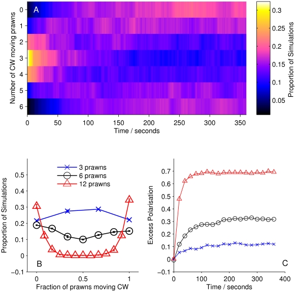
The models incorporating a non-Markovian delayed response together with a spatial interaction zone (models D1–D4) outperformed the Markovian spatial models (Figure 3) as well as the Mean Field model. Model D1 was the optimal model from those tested, indicating a symmetric short range interaction zone and interactions with only opposite oriented individuals (Table 1). Simulations of this model produce weak global consistency. Most six-prawn simulations have either five or six prawns moving in the same direction in the final state (Figure 7A). This alignment is weaker than seen in the real experiments but more consistent with the observed behaviour than any of the Markovian models. In the final distributions (Figure 7B) and mean polarisation plot (Figure 7C) we see the same increase in alignment with increasing group size as in the experimental data.

Figure 7. Simulation results for model D1.

(A) Proportion of six-prawn simulations () of non-Markovian model D1 with a given number of prawns moving CW over time, showing weak bifurcation to either a CW or an anti-CW polarised state, with most experiments ending with five or six prawns travelling in the same direction. (B) Final distribution of simulations by number of CW moving prawns for simulations with three, six and twelve prawns. Error bars represent the mean and standard deviation for each proportion as calculated from the final ten seconds of the simulations. (C) The average polarisation over time, adjusted by the expected polarisation of randomly oriented prawns, for simulations of three, six and twelve prawns. The KL divergence between the experimental and simulated results is 2.32 bits.

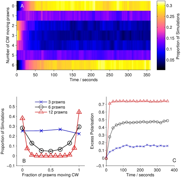
The difference in marginal likelihood between model D3 and model D1 is within the error of the sampling method, and therefore D3 should be considered as an alternative optimal model. Moreover, model D3 is globally more consistent with experiments when simulated. Figure 8A–C give the results of simulations from this model, showing a much stronger bifurcation in the prawn directions over time (Figure 8A), and more accurate scaling with group size (Figure 8B and C).

Figure 8. Simulation results for model D3.

(A) Proportion of six-prawn simulations () of non-Markovian model D3 with a given number of prawns moving CW over time, showing rapid bifurcation to either a CW or an anti-CW polarised state, with most experiments ending with six prawns travelling in the same direction. (B) Final distribution of simulations by number of CW moving prawns for simulations with three, six and twelve prawns. Error bars represent the mean and standard deviation for each proportion as calculated from the final ten seconds of the simulations. (C) The average polarisation over time, adjusted by the expected polarisation of randomly oriented prawns, for simulations of three, six and twelve prawns. The KL divergence between the experimental and simulated results is 1.46 bits.

For each model we report a measure of large-scale consistency with the experimental results, in terms of the final distribution of the proportion of CW-moving prawns. We use the Kullback-Leibler (KL) divergence [30] to measure the distance from the experimental distribution to the simulated distribution, summed over three, six and twelve prawns results (reported in Table 1 and Figures 4, 6, 7 and 8). This goodness-of-fit measure indicates that of the models discussed, the Mean Field model and non-Markovian model D3 are most consistent with the large-scale results, non-Markovian model D1 is somewhat less consistent and Markovian model S2 is very inconsistent.

Discussion

A number of physical [31]–[33], technological [34] and biological systems, including animals [9]–[11], [35], tissue cells [12], microorganisms [13], [36] are known to increase their collective order with density. Glass prawns are one additional example of such a system, which is particularly interesting since they are not known as gregarious or social species. By confining the prawns to a ring we facilitated their interactions and in doing so generated collective motion. This adds further support to the idea that collective motion is a universal phenomenon independent of the underlying interaction rules [3], [11], [37]. While we do not expect that prawns often find themselves confined in rings in a natural setting, they and other non-social animals do aggregate in response to environmental features such as food and shelter. Such environmental aggregations can, above a certain density, result in an apparently ‘social’ collective motion.

The true value of this study, however, is found not in the addition of one more species to this growing list, but in demonstrating a rigorous methodology for selecting an optimal and multi-scale consistent model for the interactions between individuals in a group. We have used a combination of techniques to identify the optimal model for our experiments: Bayesian model selection and validation against global properties. We applied Bayesian model selection to identify the model that best predicts the fine-scale interactions between prawns. This approach allows us to perform model selection in the presence of many competing hypotheses of varying complexity, while avoiding over fitting [17]. The selected models indicate that interactions between prawns are modulated primarily by the spatial separation of individuals and are localised to a very short perceptual range which is symmetric about the focal individual. This may indicate that physical contact rather than vision is the dominant mechanism, especially as the inferred size interaction zone (approximately radians) is consistent with the average body length of the prawns (approximately radians). Since in the optimal models the interaction zone is symmetric and the tracking algorithm detects a point approximately midway along the prawn's length, this suggests that the prawns may interact for as long as they remain in physical contact.

The other approach we have employed in validating our model is consistency with large-scale dynamics. Reproduction of the large-scale dynamics is frequently used to validate mathematical models of biological systems, but presents only a necessary and not a sufficient condition for model validation. Indeed, all of the models we have assessed in this work can, with the appropriate parameters, generate aligned motion consistent with experiment. The fact that our mean-field model reproduces global dynamics, but fails at a fine scale level is not particularly surprising. Mean-field models are not designed to reproduce spatially local dynamics [1]. More illuminating, however, is the failure of Markovian spatial models to the reproduce the polarisation seen in the empirical data. Models S1–S4 are variants of the standard one dimensional Vicsek self-propelled particle model [38], which has previously been validated against the global alignment patterns of marching locusts [11]. For the prawns, model parameter values which produce simulations consistent with global alignment patterns were not consistent with those inferred from fine scale observations. This inconsistency allowed us to reject standard self-propelled particle models as a good model of the data.

To identify a better model we first visually inspected the interactions between the prawns. These observations suggested a ‘memory effect’, whereby a prawn would remain influenced by individuals beyond the moment of interaction. The resulting models, D1–D4, are both consistent with the polarisation condition and superior at predicting the fine-scale interactions, providing strong evidence for non-Markovian dynamics within this system. More generally, we would expect other examples of animal motion to be non-Markovian, with individuals taking time to react to others, to complete their own actions and also potentially reacting through memory of past situations. In this context, it is important to consider the limitations of recent studies identifying rules of interaction of fish [18], [19]. These studies concentrated on quantifying local interactions, but do not try to reproduce global properties. It may be that non-Markovian and other effects are needed to produce these properties.

In what circumstances can we expect non-Markovian effects to play an important role in collective behaviour? Inference based on a Markovian model must account for behavioural changes of a focal individual in terms of their current environment. As such the crucial factor is how much the local environment changes between when the animal receives information and when it responds. Large changes in the local environment can be caused by long response times or by rapid movements of other animals relative to the focal individual. Where behavioural changes are strongly discontinuous, such as the binary one-dimensional movement in this study, non-Markovian effects may become especially important. This is because the focal individual may have to execute a number of small changes (such as stopping and turning through a several small angles) in order to register as having changed its direction of motion. Over the course of making many adjustments the environment can change dramatically from the moment that the change was initiated.

We have used qualitative replication of the large scale motion as a necessary condition for the correct model, and assigned zero probability to inconsistent models. A more subtle approach would be to give a weighting to global consistency. For example, D1 and D3 are both consistent at a global level and indistinguishable according to marginal-likelihood. As such, they should then be considered as equally viable alternative models for the real behaviour of the prawns. However, a visual inspection of global consistency favours D3 over D1 (see Figures 7 and 8). Future work could attempt to define a probability distribution over large scale outcomes, allowing fully probabilistic integration of both fine scale and large scale inference. A ‘distance’ between the summary statistics of large scale simulated behaviour and the same statistics extracted from experimental data, such as the KL divergence measure reported here, could be used to construct a Bayesian inference framework [39]. The research presented here provides a first step towards the use of multi-scale inference in the study of collective animal behaviour and in other multi-level complex systems.

Materials and Methods

Glass prawns (Paratya australiensis) were collected from Manly Dam, Sydney, Australia and transported back to aquaria facilities at the University of Sydney. They were held in 20 glass aquaria and fed green algae and fish food ad libitum. Prawns were housed for at least 2 days prior to experimentation. An annulus arena (200 mm external diameter, 70 mm internal diameter) was constructed from white plastic and filled to a depth of 25 mm with freshwater. The arena was visually isolated inside an opaque white box and filmed from above using a G10 Canon digital camera at a frame rate of 15 Hz. Data was subsequently down-sampled to 7.5 Hz by removing every second frame for computational efficiency. For each trial, we haphazardly selected one, three, six or twelve prawns and placed them in the arena. We filmed each trial for six minutes, after which we removed the prawns, emptied, and then refilled the arena with freshwater. Prawns were only used once on each day of trials. A schematic of this setup is shown in Figure 1.

Hidden Markov model

The frame-by-frame movements of the prawns are imperfect representations of the true orientation, since a prawn will often stop or even drift slightly backwards without physically turning around. A Hidden Markov Model (HMM) allows the underlying orientation of the prawns to be discovered from the noisy frame-by-frame movements by demanding a higher degree of ‘evidence’ for a direction change, in essence only identifying direction changes when the prawn makes a sustained movement in the new direction. This gives a better estimate of the true orientation than given by the instantaneous velocity alone.

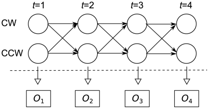
We constructed a two-state HMM [40] for the observed changes in position of the prawn, as shown in Figure 9. The two states represent clockwise (CW) or anti-clockwise (anti-CW) orientation. In a CW oriented state it is assumed that the prawn will normally move in CW direction over the course of one frame, but because the prawns movements are noisy it may move in the reverse direction over short time periods while remaining oriented CW. We model the distribution of these movements as a Gaussian distribution. We further assume a symmetrical model, such that the distribution of movements in the CW state is anti-symmetric to the distribution of movements in the anti-CW state. Thus a movement of zero is equally probable in either state. We use the Baum-Welch algorithm [40], [41] to learn the transition probability and the mean and standard deviation of the Gaussian observation probability distribution, using data from single-prawn experiments. We then apply this learnt model to identify the most probable state sequence for each of the prawns in the three-, six- and twelve-prawn experiments, using the Viterbi algorithm [40], [42].

Figure 9. Graphical description of a two-state Hidden Markov Model.

At any point in time the prawn is in a state of either CW or anti-CW orientation. The precise state is hidden but we make observations , the actual frame-by-frame movements of the prawn, which give information about the relative probabilities of the two states. We assume a fixed probability of transition between the states which is inferred from the data and allows for the persistence of orientation over time.

Calculation of marginal likelihoods

A given model, describes the probability of a change of direction for the focal prawn at time , conditioned on the current, and potentially past, positions of the other prawns, and and the parameters of the model . The likelihood for a given parameter set of the model is the probability of the data, , conditioned on the parameters and the model and is the product over both time steps and focal prawns of the probability for the observed outcome - either a change of direction or no change. Let equal one when prawn in experiment changes direction at time , and is zero otherwise, then,

(8)

where and indicate the number of experiments and the number of prawns in each experiment respectively. The marginal likelihood of the model is given by integration over the space, , of unknown parameters,

(9)

The prior distribution of the parameters, is chosen to represent the available knowledge about the parameters before the experiments and is split into independent parts. The prior for the same parameter over different models is the same to allow fair comparison.

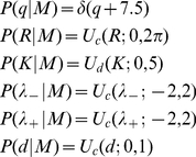(10)

where indicates a continuous uniform distribution, indicates a discrete uniform distribution and is the Dirac delta function. Numerical integration over the appropriate parameters was performed using importance sampling (see Mackay [29] Chapter 29), with 10,000 parameter samples generated from the prior parameter distribution. The importance sampling was repeated ten times for each model to improve estimates of the marginal likelihood and provide an estimate of the associated uncertainty.

References

- 1.Sumpter D. 2010. (2010) Collective Animal Behavior. Princeton University Press. URL http://www.collective-behavior.com/
- 2.Couzin ID, Krause J, James R, Ruxton GD, Franks NR. Collective memory and spatial sorting in animal groups. J Theor Biol. 2002;218:1–11. doi: 10.1006/jtbi.2002.3065. [DOI] [PubMed] [Google Scholar]
- 3.Vicsek T, Zafiris A. Collective motion. 2010. ArXiv arXiv:1010.5017v1.
- 4.Giardina I. Collective behavior in animal groups: theoretical models and empirical studies. HFSP J. 2008;2:205–219. doi: 10.2976/1.2961038. [DOI] [PMC free article] [PubMed] [Google Scholar]
- 5.Czirόk A, Barabási A, Vicsek T. Collective motion of self-propelled particles: Kinetic phase transition in one dimension. Phys Rev Lett. 1999;82:209–212. [Google Scholar]
- 6.Vicsek T, Czirόk A, Ben-Jacob E, Cohen I, Shochet O. Novel type of phase transition in a system of self-driven particles. Phys Rev Lett. 1995;75:1226–1229. doi: 10.1103/PhysRevLett.75.1226. [DOI] [PubMed] [Google Scholar]
- 7.Huth A, Wissel C. The simulation of the movement of fish schools. J Theor Biol. 1992;156:365–385. [Google Scholar]
- 8.Str̈ombom D. Collective motion from local attraction. J Theor Biol. 2011;283:145–151. doi: 10.1016/j.jtbi.2011.05.019. [DOI] [PubMed] [Google Scholar]
- 9.Becco C, Vandewalle N, Delcourt J, Poncin P. Experimental evidences of a structural and dynamical transition in fish school. Physica A. 2006;367:487–493. [Google Scholar]
- 10.Beekman M, Sumpter D, Ratnieks F. Phase transition between disordered and ordered foraging in pharaoh's ants. Proc Natl Acad Sci U S A. 2001;98:9703–9706. doi: 10.1073/pnas.161285298. [DOI] [PMC free article] [PubMed] [Google Scholar]
- 11.Buhl J, Sumpter D, Couzin I, Hale J, Despland E, et al. From disorder to order in marching locusts. Science. 2006;312:1402–1406. doi: 10.1126/science.1125142. [DOI] [PubMed] [Google Scholar]
- 12.Szabo B, Szollosi GJ, Gonci B, Juranyi Z, Selmeczi D, et al. Phase transition in the collective migration of tissue cells: Experiment and model. Phys Rev E. 2006;74:061908. doi: 10.1103/PhysRevE.74.061908. [DOI] [PubMed] [Google Scholar]
- 13.Sokolov A, Aranson IS, Kessler JO, Goldstein RE. Concentration dependence of the collective dynamics of swimming bacteria. Phys Rev Lett. 2007;98:158102. doi: 10.1103/PhysRevLett.98.158102. [DOI] [PubMed] [Google Scholar]
- 14.Ballerini M, Cabibbo N, Candelier R, Cavagna A, Cisbani E, et al. Interaction ruling animal collective behavior depends on topological rather than metric distance: Evidence from a field study. Proc Natl Acad Sci U S A. 2008;105:1232–1237. doi: 10.1073/pnas.0711437105. [DOI] [PMC free article] [PubMed] [Google Scholar]
- 15.Lukeman R, Li Y, Edelstein-Keshet L. Inferring individual rules from collective behavior. Proc Natl Acad Sci U S A. 2010;107:12576. doi: 10.1073/pnas.1001763107. [DOI] [PMC free article] [PubMed] [Google Scholar]
- 16.Eriksson A, Nilsson Jacobi M, Nyström J, Tunström K. Determining interaction rules in animal swarms. Behav Ecol. 2010;21:1106–1111. [Google Scholar]
- 17.Mann RP. Bayesian inference for identifying interaction rules in moving animal groups. PLoS ONE. 2011;6:e22827. doi: 10.1371/journal.pone.0022827. [DOI] [PMC free article] [PubMed] [Google Scholar]
- 18.Katz Y, Ioannou C, Tunstrom K, Huepe C, Couzin I. Inferring the structure and dynamics of interactions in schooling fish. Proc Natl Acad Sci U S A. 2011;108:18720–18725. doi: 10.1073/pnas.1107583108. [DOI] [PMC free article] [PubMed] [Google Scholar]
- 19.Herbert-Read JE, Perna A, Mann RP, Schaerf T, Sumpter DJT, et al. Inferring the rules of interaction of shoaling fish. Proc Natl Acad Sci U S A. 2011;108:18726–18731. doi: 10.1073/pnas.1109355108. [DOI] [PMC free article] [PubMed] [Google Scholar]
- 20.Yates C, Erban R, Escudero C, Couzin I, Buhl J, et al. Inherent noise can facilitate coherence in collective swarm motion. Proc Natl Acad Sci U S A. 2009;106:5464. doi: 10.1073/pnas.0811195106. [DOI] [PMC free article] [PubMed] [Google Scholar]
- 21.Bode N, Faria J, Franks D, Krause J, Wood A. How perceived threat increases synchronization in collectively moving animal groups. Proc Roy Soc B. 2010;277:3065. doi: 10.1098/rspb.2010.0855. [DOI] [PMC free article] [PubMed] [Google Scholar]
- 22.Hoare D, Couzin I, Godin J, Krause J. Context-dependent group size choice in fish. Anim Behav. 2004;67:155–164. [Google Scholar]
- 23.Sumpter D, Krause J, James R, Couzin I, Ward A. Consensus decision making by fish. Curr Biol. 2008;18:1773–1777. doi: 10.1016/j.cub.2008.09.064. [DOI] [PubMed] [Google Scholar]
- 24.Williams WD. Some aspects of the ecology of paratya australiensis. Aus J Mar Fresh Res. 1977;28 [Google Scholar]
- 25.Jeffreys H. Theory of Probability. Oxford University Press; 1939. [Google Scholar]
- 26.Berger J. Statistical decision theory and Bayesian analysis. Springer; 1985. [Google Scholar]
- 27.Jaynes E. Probability Theory. New York: Cambridge University Press; 2003. [Google Scholar]
- 28.Bernardo JM, Smith AFM. Bayesian Theory. Wiley; 2007. [Google Scholar]
- 29.MacKay DJC. Information Theory, Inference and Learning Algorithms. Cambridge University Press; 2003. [Google Scholar]
- 30.Kullback S, Leibler RA. On information and sufficiency. Ann Math Stat. 1951;22:79–86. [Google Scholar]
- 31.Bloustine J. Experimental investigations into interactions and collective behavior in protein/polymer mixtures and granular rods. [Ph.D. thesis] Boston (Massachusetts): Brandeis University; 2006. [Google Scholar]
- 32.Kudrolli A, Lumay G, Volfson D, Tsimring L. Swarming and swirling in self-propelled polar granular rods. Phys Rev Lett. 2008;100:58001. doi: 10.1103/PhysRevLett.100.058001. [DOI] [PubMed] [Google Scholar]
- 33.Ginelli F, Peruani F, Bär M, Chaté H. Large-scale collective properties of self-propelled rods. Phys Rev Lett. 2010;104:184502. doi: 10.1103/PhysRevLett.104.184502. [DOI] [PubMed] [Google Scholar]
- 34.Tarcai N, Viragh C, Abel D, Nagy M, Varkonyi PL, et al. Patterns, transitions and the role of leaders in the collective dynamics of a simple robotic flock. J Stat Mech-Theory E. 2011:P04010. [Google Scholar]
- 35.Buhl J, Sword GA, Clissold FJ, Simpson SJ. Group structure in locust migratory bands. Behav Ecol Sociobiol. 2011;65:265–273. [Google Scholar]
- 36.Wua Y, Kaiser AD, Jiang Y, Alber MS. Periodic reversal of direction allows myxobacteria to swarm. Proc Natl Acad Sci U S A. 2009;106:1222–1227. doi: 10.1073/pnas.0811662106. [DOI] [PMC free article] [PubMed] [Google Scholar]
- 37.Grunbaum D. Behavior - align in the sand. Science. 2006;312:1320–1322. doi: 10.1126/science.1127548. [DOI] [PubMed] [Google Scholar]
- 38.Czirok A, Barabasi A, Vicsek T. Collective motion of self-propelled particles: Kinetic phase transition in one dimension. Phys Rev Lett. 1999;82:209–212. [Google Scholar]
- 39.Toni T, Welch D, Strelkowa N, Ipsen A, Stumpf M. Approximate bayesian computation scheme for parameter inference and model selection in dynamical systems. J Roy Soc Interface. 2009;6:187. doi: 10.1098/rsif.2008.0172. [DOI] [PMC free article] [PubMed] [Google Scholar]
- 40.Rabiner L. A tutorial on hidden Markov models and selected applications in speech recognition. Readings in speech recognition. 1990;53:267–296. [Google Scholar]
- 41.Baum L, Petrie T, Soules G, Weiss N. A maximization technique occurring in the statistical analysis of probabilistic functions of markov chains. Ann Math Stat. 1970;41:164–171. [Google Scholar]
- 42.Viterbi A. Error bounds for convolutional codes and an asymptotically optimum decoding algorithm. IEEE T Inform Theory. 1967;13:260–269. [Google Scholar]