Abstract
Purpose
To characterize cardiac motion artifacts in the liver and assess the use of a post-processing method to mitigate these artifacts in repeat measurements.
Materials and methods
Three subjects underwent breathhold diffusion-weighted (DW) scans consisting of 25 repetitions for three b-values (0, 500, 1000 sec/mm2). Statistical maps computed from these repetitions were used to assess the distribution and behavior of cardiac motion artifacts in the liver. An objective post-processing method to reduce the artifacts were compared with radiologist-defined gold standards.
Results
Signal dropout is pronounced in areas proximal to the heart, such as the left lobe, but also present in the right lobe and in distal liver segments. The dropout worsens with b-value and leads to overestimation of the diffusivity. By reference to a radiologist-defined gold standard, a post-processing correction method is shown to reduce cardiac motion artifact.
Conclusion
Cardiac motion leads to significant artifacts in liver DW imaging; we propose a post-processing method that may be used to mitigate the artifact and is advantageous to standard signal averaging in acquisitions with multiple repetitions.
Keywords: diffusion-weighted MRI, liver, cardiac motion, artifact
Introduction
With continuing technical advances, diffusion-weighted (DW) magnetic resonance imaging (MRI) of the liver has become commonplace. A growing body of work has shown the potential of using diffusion parameters as biomarkers of diffuse liver disease (1–3). According to the current understanding of diffusion in the liver, the DW signal reflects perfusion (D*) and diffusion (D) components through an intravoxel incoherent motion model (4):
| [1] |
where S and S0 represent the signal intensity with and without the diffusion gradients, b (also referred to as b-value) is a measure of the area of the motion-sensitizing gradients, and perfusion fraction PF is the signal fraction of the intravascular component. Equation 1 is sometimes approximated as a monoexponential decay:
| [2] |
where the apparent diffusion coefficient (ADC) contains a mixture of the contributions from D* and D.
By measuring the parameters in the diffusion signal equations (Eqns. 1 and 2), it is possible to assess physical changes in organs. However, application of DW imaging to the liver thus far has produced somewhat inconsistent results, with one group reporting no significant difference in diffusion parameters between cirrhotic and normal livers (3), another group reporting that cirrhotic livers had decreased ADC and D* compared to normal livers but no difference in D values (1), and yet another group reporting that cirrhotic livers had decreased ADC, D* and D values compared to normal livers (2). These partly conflicting results are likely due to differences in experimental paradigms, such as selection of b-values, use of monoexponential (Eqn. 2) versus biexponential (Eqn.1) models (5), and methods used to account for the impact of physiological noise (i.e. respiratory and cardiac motion) on measurements. In order for DW imaging to be used reliably for clinical assessment of liver disease, it is critical to develop a methodology that yields reproducible results.
While respiratory motion is well known and has been addressed in prior studies (6–9), there is relatively less literature on the effects of cardiac motion. Diffusion gradients are designed to sensitize images to motion on a molecular and microscopic level, so minor bulk motion in the liver caused by cardiac motion can lead to anecdotal clinical observations of variable signal dropout in the left lobe proximal to the heart. A recent study demonstrated that cardiac motion artifacts are also present in the right liver lobe although to a lesser degree (10). Since the signal loss is proportionate to the motion sensitization, it leads to an artifactual decrease in the measured signal with b-value and hence an overestimation of diffusion parameters (ADC, D*, D). The link between cardiac motion and DW image artifacts was first established by using cardiac gating to show that images acquired in cardiac diastole had less motion artifacts than those acquired in systole (11). Prior studies sought to account for the effects of cardiac motion by cardiac gating, exclusion of the left liver lobe from measurements, or employing visual screening of the data. Cardiac gating is an imperfect solution to the problem of cardiac motion in DW imaging because the short acquisition window limits the number of slices and number of b-values. Exclusion of the left liver lobe (2,8,12) is obviously not ideal because it neglects the presence of disease in a large portion of the liver. Employing visual screening of data for artifacts prior to calculation of diffusion parameters (13) is subjective and is unlikely to be practical in a clinical setting. Thus, the development of an objective method to reduce the effects of cardiac motion would be helpful to improving liver diffusion examinations.
There are two purposes in this study: 1) To characterize the distribution and statistical behavior of cardiac motion artifacts in the liver, and 2) To assess the use of a post-processing method to mitigate cardiac motion artifacts in repeat measurements.
Materials and Methods
Experimental protocol
Three healthy adult subjects (1 female, 2 males, ages 30, 33, 66 years) participated in the study after giving informed consent. The MRI examinations were performed on a high-performance gradient (maximum gradient 40 mTm−1; maximum slew rate, 150 Tm−1s−1) 3T Twin-speed MRI scanner (GE Healthcare, Milwaukee, WI, USA) equipped with an eight-element body phased array coil. All subjects were scanned in supine position. A respiratory belt was applied to monitor the breathing cycle, and subjects were instructed to suspend respiration during the image acquisition. A dielectric pad was placed between the coil and the abdominal wall.
MRI sequences
Breathhold DW images were obtained using a customized DW spin-echo echo-planar-imaging (SE EPI) sequence (14). A pair of trapezoidal gradient pulses was applied along a single diffusion direction, which was the vector sum of the three physical gradients. We applied the following parameters for each breathhold DW scan: axial imaging plane, flip angle = 90°, TR = 1500ms, TE = 45ms, matrix size = 160 × 128 zero-padded to 256 × 256, slice thickness = 8–9mm, intersection gap = 9–10mm, number of slices 9–10, receive bandwidth = 1953 Hz/pixel, number of averages = 1, spectral-spatial water excitation, and parallel imaging factor = 2. Each scan consisted of 29 repetitions and lasted 42 seconds with all repetitions acquired in the same breathhold. The first 4 repetitions used b = 0 sec/mm2 to ensure constant gain settings between scans and ensure the magnetization was at steady state and were discarded. The remaining 25 repetitions used one of three designated b-values (0, 500, 1000 sec/mm2).
Data analysis
The 25 repeat measurements were intended to sample different phases of the cardiac cycle and to reflect the common practice of acquiring multiple repeats (averages) to improve signal-to-noise ratio and/or reduce artifacts. A post-processing method referred to in this study as the p-mean was used to combine repeat measurements:
| [3] |
where y is the p-mean, n is the number of samples, x is the pixel value and power is the exponent. When power > 1, higher pixel values are emphasized and introduces a small positive bias when the data has normally distributed error. However the assumption of normally distributed error is clearly violated in DW images, where data contains signal dropout from cardiac motion. Standard averaging (corresponding to a power=1), incorporates the signal dropout as a negative bias. The goal of using a different power is to avoid this potentially large negative bias at a cost of introducing a small positive bias when the artifact is absent.
Calculations and data analyses were performed using custom-written Matlab software (The MathWorks, Natick, MA, USA). Curve-fitting of DW parameters was performed using nonlinear least squares.
Cardiac motion artifact characterization
Statistical maps of the mean and standard deviation in each voxel were formed for the 25 consecutively acquired images for each b-value, subject, and slice. Circular regions-of-interest (ROIs), approximately 480 voxels, were drawn on the left and right liver lobes of a superior slice for each subject. Care was taken to position the ROIs away from liver edges and areas of partial voluming.
Image Quality Assessments
Images were formed by computing the per-voxel p-mean from the first ten consecutive images of each scan for power values 1 to 8 (Eqn. 3). The per-voxel maximum was also taken to form the maximum image, which is equivalent to power=∞ To assess the quality of these images, two approaches were adopted
Firstly, two board-certified radiologists with 6 and 1 years of experience made blinded assessments of the 9 differently combined images in 3 subjects and 9 slices (total 2×9×3×9=486 independent evaluations) at b = 1000 sec/mm2 to determine which power value provided the highest quality images. The anticipated trade-off communicated to the radiologists was between signal dropout and higher noise in the images.
Secondly, numerical differences were measured between a “gold standard” image with the images produced from different powers. The gold standard image was created by asking the radiologists to select 5 images from the 25 repeated images that were least corrupted by cardiac motion artifact. The average (power = 1) of the five images formed a gold standard image. We then randomly selected 10 images from the 25 images in the same scan (groups of 10 random instead of consecutive images were used to allow comparisons to be run multiple times) and computed images with power ranging from 0.25 to 10 in increments of 0.25. A pixel-by-pixel root mean squared error (RMSE) was performed with the gold standard image for each power value; lower RMSE indicated a better match. This was performed 1,000 times for a superior and inferior slice for each subject and b-value. Although having a greater number of repetitions/images is clearly more desirable for statistics and to ensure equal representation of cardiac cycle phases, the maximum number is limited by experiment length, subject fatigue, and breathhold capability. We recommend acquisition of as many repetitions as experimental design allows and use 10 images here as an example of what reasonably may be acquired.
Parameter Estimation Assessments
To assess the effect of the p-mean combination method on diffusion parameter estimates, we computed the per b-value p-mean by taking the p-mean with power=4 of the 25 per repetition signal intensities for each ROI, b-value, and subject. Fitting the signal versus b-value to a monoexponential decay produced ADC estimates (Eqn. 2). This was repeated for the power=1 and for the gold standard data. Two-tailed paired t-tests were used to compare the three sets of ADC estimates.
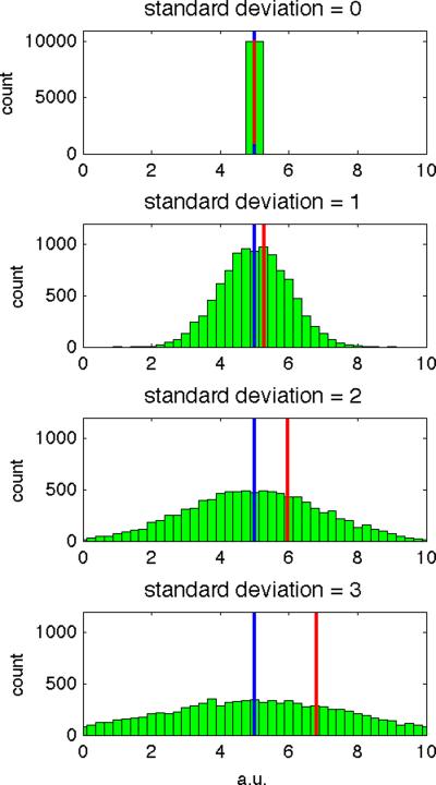
Additional noise simulations were performed to determine how differences in the sample standard deviation affect the size of the bias as a function of power. Four sets of 10,000 normally distributed random samples were generated with a mean of 5 and standard deviations of 0, 1, 2, and 3. The mean (power=1) and p-mean (power=4) were computed for each set. To asses the effects of p-mean on real data with minimal artifacts, it was applied with power=4 to the gold standard data.
Results
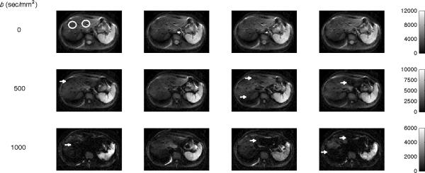
Figure 1 shows four consecutive liver DW images obtained with b = 0 (top row), 500 (middle row), and 1000 sec/mm2 (bottom row) from Subject 1. When b=0 sec/mm2 (no motion sensitization gradient) there is not expected to be any signal dropout from cardiac motion. Consistent with expectations, the liver parenchyma appears homogeneous and unchanged between repeats. Differences are visible in the aorta, which reflect the phase of the cardiac cycle. At b=500 sec/mm2, dark patches from cardiac motion artifact are visible in the liver parenchyma in different locations between repeats (indicated by arrows). The liver parenchyma in a couple images appears homogeneous and well-intact (middle row, second image), while the left liver lobe of another image is largely obscured (middle row, fourth image). At b=1000 sec/mm2, multiple dark patches in the liver parenchyma are present in each image. The cardiac motion artifacts worsen with b-value and tend to be more prominent proximal to the heart (left liver lobe), but are also present in the right liver lobe. The precise location of the artifact is inconsistent between repeats.
Figure 1.
Liver DW images across b-values for Subject 1. Four consecutive liver DW images obtained with b = 0 (top row), 500 (middle row), and 1000 (bottom row) sec/mm2. With no diffusion weighting (top row), all images are similar except for the different amounts of blood contained in large vessels such as the aorta. In the high b-values images, areas of patchy image dropout are seen (indicated by arrows) that worsen with increased diffusion weighting and are most pronounced in the left liver lobe. The white circles show examples of typical ROI placements.
Figure 2 shows statistical maps of the mean (left column) and standard deviation (right column) computed voxel-wise from all 25 repeats of one slice for Subject 1. In the left column, the mean visibly decreases with increasing b-value, consistent with DW signal dephasing from micro- and macroscopic motion. In the right column and top row, the standard deviation is minimal in the b=0 sec/mm2 image and relatively uniform except in large vessels such as the aorta and at organ edges. The increased standard deviation in large vessels is due to the different phases of the cardiac cycle in each consecutive image, as noted in Figure 1. The increased standard deviation at organ edges is likely the result of thoracic and abdominal muscle relaxation throughout the breathhold acquisition. At b=500 sec/mm2, areas of high standard deviation are seen in the left liver lobe, stomach, and at organ edges. Large vessels are no longer enhanced because signal from flowing blood is rapidly dephased at this b-value. The high standard deviation in the left liver lobe is consistent with the dark patches intermittently present in the left liver lobe of Figure 1. At b=1000 sec/mm2, areas of increased standard deviation extend to the right liver lobe and spleen. In ROIs placed in the liver there was a dramatic increase in the standard deviation in the left lobe from b = 0 to 500 sec/mm2 (+223%) and from b = 0 to 1000 sec/mm2 (+92%). Consistent with the finding of fewer cardiac artifacts the right liver lobe, the standard deviation increases in the right lobe were comparatively smaller for b = 0 to 500 sec/mm2 (+46%) and b = 0 to 1000 sec/mm2 (+39%). Cardiac motion artifacts are expected to be highest at the greatest b-value (b=1000). However, the standard deviation of b=1000 is smaller than b=500 due to the combination of low mean values and the lower bound of 0 (Rician-like noise distribution), so the full variability in the data is not seen.
Figure 2.
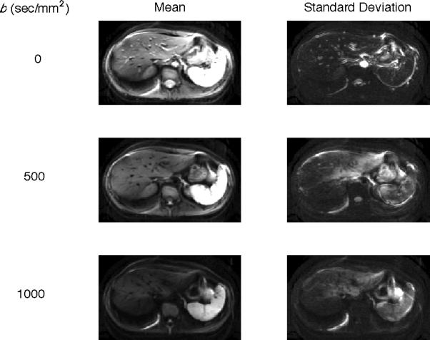
Statistical maps for Subject 1 across b-values. Statistics are computed pervoxel for the 25 consecutively acquired DW images at b = 0 (top row), 500 (middle row) and 1000 (bottom row) sec/mm2. The mean signal intensity (left column) decreases with increasing b-value, consistent with DW theory. The standard deviation of the signal intensity (right column) is greatest in areas of pulsatile blood flow in b = 0 sec/mm2images and in areas proximal to the heart in the b = 500 and 1000 sec/mm2 images.
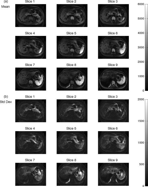
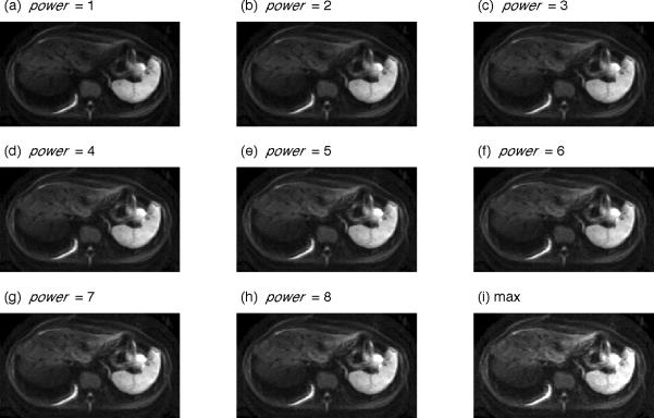
Figure 3 shows statistical maps computed from the 25 images from each slice of Subject 1 at b=1000 sec/mm2 to illustrate spatial changes across slices. In the mean images (Figure 3a), the liver parenchyma has generally less signal in the medial portions of the superior slices. The standard deviation maps (Figure 3b) show highest signal variability in areas proximal to the heart and at organ edges, as noted in Figure 2. Regions of decreased mean signal and increased standard deviation in the liver are found in all displayed slices, indicating that signal dropout is present even in distal segments. Figure 4 describes the results of imaging experiments, in which multiple repeats are commonly acquired to increase the signal-to-noise ratio and reduce artifacts. As noted in the Introduction, averaging these data presumes a symmetric error distribution whereas in DW imaging the error favors low values. Panels (a)–(i) show images created from Eq 3 with increasing power value computed from 10 repeats of Subject 1's b=1000 sec/mm2 data. Note the dark patch in the left lobe of the mean image (power=1, panel (a)) is progressively reduced with increasing power value. Simultaneously, the background noise increases with increasing power value and is most pronounced in the maximum image (power=∞). Intermediate power values provide a trade-off between decreasing cardiac motion artifact and increasing background noise.
Figure 3.
Statistical maps for Subject 1 at b = 1000 sec/mm2 across slices. Statistics are computed per-voxel for the sets of 25 consecutively acquired DW images. Slices are positioned from inferior (slice 1) to superior (slice 9) showing the voxel-wise (a) mean and (b) standard deviation. Areas of increased standard deviation in the liver are present in all displayed slices and are pronounced in areas proximal to the heart, reflective of the patchy signal loss due to cardiac motion.
Figure 4.
p-mean images for Subject 1 computed for b=1000 sec/mm2 images. The pervoxel p-mean is computed from 10 consecutively acquired images for the indicated power values (a) – (h) and for power=∞ (i). Areas of signal loss, particularly in the left liver lobe, are lessened with increasing power value. As illustrated in the maximum image, background noise dominates at high power values.
In the first qualitative evaluation (described in Methods), two board-certified radiologists who were blinded to the power visually assessed image quality in a total of 243 images each. The first radiologist determined power=5.0 (std 2.2, range 1 – 8, S1=5.3, S2=3.4, S3=6.4 where S is subject) as the mean preferred value. The second radiologist determined power=3.4 (std 2.5, range 1 – 8, S1=3.2, S2=1.4, S3=5.6) as the mean preferred value.
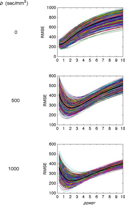
In the second evaluation, radiologist-defined gold standards were numerically compared with images produced with different powers (details in Methods). Figure 5 shows a representative example of the root mean squared error (RMSE, y-axis) versus the power value (x-axis) between the gold standard and 1000 random subsets of the images (Subject 1, superior slice). The averages of these RMSEs for each b-value are overlaid in the thick black line. The RMSEs vary smoothly across the range of power values and reach a minimum at intermediate power values.
Figure 5.
Simulation results comparing gold standard images and p-mean images for Subject 1. The root mean squared error (RMSE, y-axis) is plotted against the power value (x-axis) for 1000 examples (thin lines) and the mean of the 1000 examples (thick black lines) for b = 0 (top row), 500 (middle row), and 1000 (bottom row) sec/mm2. The power value that produces the minimum RMSE between the gold standard and p-mean images increases with increasing b-value.
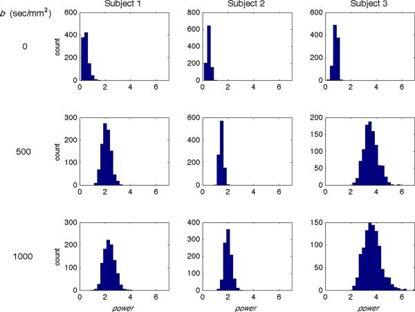
Figure 6 shows histograms of the optimal power values for the 1000 RMSE trials for each subject and b-value. The optimal values increase with b-value for all subjects (Subject 1: 0.47, 2.11, 2.32; Subject 2: 0.49, 1.47, 1.99; Subject 3: 0.81, 3.57, 3.68 for b = 0, 500 and 1000 sec/mm2, respectively). Note these values are lower than the radiologist-preferred values; while the radiologists were specifically focused on the liver parenchyma, the numerical evaluations were based on the entire field of view. Although power=1 is expected to be the optimal value for b=0, we found values to be <1. As seen in Figure 1, the main variance between b=0 images is the amount of blood in the aorta. It seems that the radiologists preferentially selected gold standard images that did not contain blood in the aorta, perhaps out of a desire for image homogeneity. This resulted in optimal power values <1 to down-weight the aorta blood and better match gold standard images. Additional simulations (not shown) with gold standards preferentially formed from images containing blood in the aorta showed optimal power values >=1.
Figure 6.
Simulation results comparing gold standard images and p-mean images for a superior slice of all subjects and b-values. Histograms show power values that produce the lowest RMSEs between the gold standard and p-mean images from 1000 trials for Subject 1 (left column), 2 (middle column), and 3 (right column) and for b = 0 (top row), 500 (middle row), and 1000 (bottom row) sec/mm2. The histogram means increase with increasing b-value for each subject.
From the above experiments, it seems that different b-values have different optimal power values and even different areas within each image may warrant a different power due to spatial variation of the artifact. The optimal power values also varied between the subjects, which may be due to differences in physiologic properties such as heart rate or viscoelastic properties of the liver parenchyma. Application of increasing power values monotonically increases the amount of positive bias, but it is impractical to use different power values for each situation. For this reason we chose power=4 as it is an integer and lies midway between the radiologist-preferred power values (3.4 and 5.0). In Figures 7 and 8, we show how use of power=4 affects DW measurements.
Figure 7.
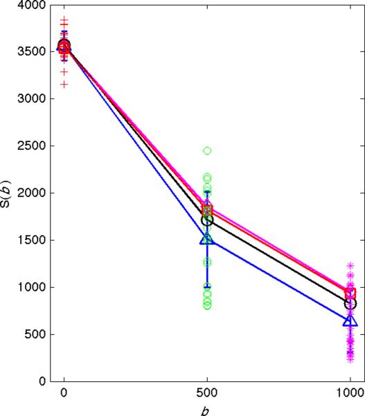
Application of p-mean to DW measurements. Signal intensity (y-axis) versus b-value (x-axis) from 10 repeated measurements in the left liver lobe are shown. Standard deviations are indicated by vertical blue lines. The arithmetic means are shown by the blue triangles, the p-mean (power=4) by the black circles, the gold standard measurements by the red squares, and the p-mean of the gold standard data by the magenta diamonds. All measurements are nearly identical when there is no cardiac noise at b = 0 sec/mm2. At higher b-values the spread of the data points increases and difference between the arithmetic means and p-means increases. In all cases, the p-mean is closer to the gold standard than the arithmetic mean. Also, the p-mean of the gold standard data is almost identical to the original gold standard data, reinforcing that data without artifacts is largely unchanged by the p-mean.
Figure 8.
Application of p-mean to DW measurements. Histograms of 10,000 normally distributed samples with arithmetic mean=5 (power=1, blue line) and standard deviation of (a) 0, (b) 1, (c) 2, and (d) 3 (arbitrary units). In each case, the p-mean to power=4 is shown (red line). As the standard deviation of the sample increases, the difference between the arithmetic and p-mean also increases, indicating positive bias in the p-mean estimator.
Figure 7 shows typical data from the left liver lobe ROI of Subject 1 with the power=1 (blue triangles) and power=4 (black circles) combinations and values obtained from the gold standard (red squares) indicated. In agreement with the simulations, the power=4 data has only a small effect on the b=0 sec/mm2 data (distance between blue triangle and black circle) but positively biases the b=500 sec/mm2 and b=1000 sec/mm2 data. Furthermore, the difference between power=4 and gold standard measurements (distance between the black circles and red squares) is smaller than the difference between the power=1 and gold standard measurements (distance between the blue triangles and red squares), indicating that the p-mean provides a better estimate of the true signal than the arithmetic mean. Also shown is the p-mean of the gold standard data with power=4 (magenta diamonds), which significantly overlaps with the original gold standard data (red squares), reinforcing that the p-mean leaves data with minimal artifacts largely unchanged.
Table 1 shows the apparent diffusion coefficient (ADC) computed with the power=1 and power=4 combinations and gold standard values for each subject. The ADC estimates computed from power=1 data were larger than those from the gold standard data in both the left (+32.0%, p=0.16) and right (+9.0%, p=0.17) liver lobes. The greater overestimation in the left versus right liver lobes is consistent with worse cardiac motion artifacts in the left liver lobe. ADC estimates from the p-mean (power=4) data were also on average larger than those computed from the gold standard data (left: +8.7%, p=0.53; right: +5.2%, p=0.36), but the overestimation is much reduced compared to the power=1 data.
Table 1.
ADC values in liver measured from ROI measurements in the right and left lobes using p-means (power = 1 and 4) and the radiologist gold standard.
| Subject | Right Lobe ADC (10−3mm2 / s) | Left Lobe ADC (10−3mm2 / s) | ||||
|---|---|---|---|---|---|---|
| power = 1 | power = 4 | Gold | power = 1 | power = 4 | Gold | |
| 1 | 0.91 | 0.87 | 0.90 | 1.70 | 1.50 | 1.30 |
| 2 | 0.89 | 0.86 | 0.75 | 1.90 | 1.60 | 1.80 |
| 3 | 1.40 | 1.40 | 1.3 | 2.40 | 1.90 | 1.50 |
Figure 8 shows histograms of 10,000 normally distributed random samples with arithmetic mean = 5 and standard deviations = 0 – 3. By computing the mean (power=1, blue line) and a p-mean (power=4, red line) for each data set, we see that the difference between the two estimates (distance between blue and red lines) increases with increasing standard deviation of the data set. Thus larger variation in the data produces a greater bias in the power=4 image. This property has the effect of leaving data without cardiac motion artifacts relatively unchanged (e.g. data with b=0 sec/mm2 has little artifact and hence a small standard deviation) compared to data exhibiting cardiac motion artifacts (e.g. data with b=500 sec/mm2 data exhibits a large standard deviation).
Discussion
The first purpose of this study was to assess signal dropout artifacts in the liver that have been attributed to cardiac motion (10,11). By acquiring multiple consecutive liver DW images at different phases of the cardiac cycle, we were able to identify areas exhibiting decreased mean and increased standard deviation. Measurements showed an increase in the standard deviation of the signal with diffusion weighting in the left liver lobe (+223% from b = 0 to 500 sec/mm2, +92% from b = 0 to 1000 sec/mm2), and in the right liver lobe (+46% from b = 0 to 500 sec/mm2, +39% from b = 0 to 1000 sec/mm2). The higher standard deviations in the left versus right liver lobes are consistent with prior studies reporting that cardiac motion artifacts are most pronounced in areas proximal to the heart (2,10–13).
We also found that cardiac motion artifacts were present in the right liver lobe, as reported by a previous study (10), and in inferior liver segments distal to the heart. The extensive presence of artifacts throughout the liver indicates that simple exclusion of the left liver lobe (2,8,12) is not a satisfactory solution.
The second purpose of this study was to assess the use of a novel approach to reduce cardiac motion artifacts in liver DW imaging, whereby repeated measurements are combined as powers according to Eq 3. Standard signal averaging may be considered equivalent to power=1, while using power>1 gives a self-weighted combination that over-represents higher signals in order to counteract signal dropout caused by cardiac motion
We observed increasing power values reduced the cardiac motion artifacts but increased noise in the images. Based on radiologist-selected gold standard images, we found that there was no single optimal power value for all cases. Instead, different b-values exhibited different degrees of cardiac motion artifact and hence required different powers to best match the gold standard, ranging from ~1 at b=0 sec/mm2 to ~4 at b=1000 sec/mm2. Since it is more practical to use a single power value across images and studies, we assessed how using power=4 for all images affected diffusion parameter measurements. We found that samples with no cardiac motion artifact were relatively unchanged while a strong positive bias was exerted on samples affected by cardiac motion. Thus, while liver ADCs were substantially overestimated using the power=1 combination in the left (+32.0%) and right (+9.0%) liver lobes, as compared to gold standard values, the use of the power=4 combination greatly reduced ADC overestimation (left +8.7%, right +5.2%).
Other combination methods may perform better and, theoretically, the use of power=∞ (i.e. maximum value) should exclude most cardiac-related dropout artifacts. In practice, however, using power=∞ is not acceptable due to the increase in noise. We recommend a compromise of computing the p-mean at low to moderate power values (i.e. power=4), which balances the trade-off between reducing cardiac motion artifact and increasing noise.
Our definition of p-mean has subtle differences from two well known mathematical formulas: the p-norm (15) and the generalized mean (16). The p-norm is very similar to the p-mean with the only difference being normalization for number of samples. The generalized mean uses signed (or complex) values whereas the p-mean and p-norm are performed on magnitude values. The magnitude operation is implicit in the image reconstruction method used here, which is tailored for a partial Fourier acquisition and gives phase-corrected images. Partial Fourier is used in many EPI implementations to reduce echo times. Standard averaging may be performed on the k-space data prior to image reconstruction, however applying the p-mean to this data is problematic, since signal dropout can only be identified in the image domain. To the authors' best knowledge it is not possible to apply a p-mean combination method to the complex k-space data, but only to the images.
Note that although the number of subjects (3) used in this study is a small, the important sample size here is the number of repeats (25), as this is the scale in which the majority of comparisons in this work are done. Breathhold capability is the main limitation to the number of repeats in this study.
The p-mean method assumes that measurements with the highest signal intensity contain the least motion artifacts, since bulk motion during diffusion-weighting leads to signal dephasing and loss. However, it is important to note this assumption may be violated when bulk motion between TRs replace voxel elements with tissues that have decreased diffusion properties or even change the position of residual chemical shift artifact. These effects may be reduced by preferentially taking measurements from within homogeneous structures away from organ edges.
A limitation of this study is that we used a breathhold paradigm. In clinical use, patients may be unable to sustain the required breathhold length for multiple DW measurements. In these cases, free-breathing may be a more practical and comfortable alternative. Bulk movement of the liver in free-breathing is much larger than the cardiac pulsation but may be less problematic in terms of signal dropout, since it is slower and the diffusion gradients are only sensitive to motion occurring over a few tens of milliseconds. A prior study using slowly moving fluid-filled phantoms to simulate respiratory motion found less than 10% error in ADC measurements in the fluid of the phantom. Their result suggests that while the uniform motion of respiration causes errors in ADC measurements of small focal lesions, large homogeneous structures such as the liver may be less affected (17,18).
Another limitation of this study is that we did not measure EKG signals. At the TR of 1500ms, data from participants with a heart rate in multiples of 40 may have been acquired from a preferred phase of the cardiac cycle. This was unlikely to have occurred with our data, as visual inspection revealed greatly different artifacts between repetitions, consistent with sampling from multiple phases of the cardiac cycle. Data sampled from a single cardiac phase would decrease the effectiveness of the p-mean method, which relies on acquiring a mixture of correct and artefactual data. Use of EKG measurements to ensure sampling of all phases would be expected to augment the correction method. However, in our initial experience with gating, we have found it difficult to find a phase of the cardiac cycle that yielded DW images free of dropout artifacts or even with a reproducible artifact.
Cardiac gating has been used to reduce cardiac motion artifacts in liver DW imaging previously (10,11). Although this is an intuitively appealing method, the impact of the heart on the liver and arterial pulsation post-systole may cause long-lived non-rigid body motion in both liver lobes (10). This may explain why the location of the cardiac motion artifacts seen in our study varied so widely between consecutive images.
In conclusion, we found that cardiac motion artifacts in liver DW imaging are not only found in areas proximal to the heart, but are also present in the right liver lobe and distal liver segments. We propose a simple post-processing method that has advantages over standard signal averaging in reducing these artifacts in scans with multiple repetitions.
Acknowledgments
Grant support: NIH R01 #DK075128.
References
- 1.Luciani A, Vignaud A, Cavet M, et al. Liver cirrhosis: intravoxel incoherent motion MR imaging--pilot study. Radiology. 2008;249(3):891–899. doi: 10.1148/radiol.2493080080. [DOI] [PubMed] [Google Scholar]
- 2.Patel J, Sigmund EE, Rusinek H, Oei M, Babb JS, Taouli B. Diagnosis of cirrhosis with intravoxel incoherent motion diffusion MRI and dynamic contrast-enhanced MRI alone and in combination: preliminary experience. J Magn Reson Imaging. 2010;31(3):589–600. doi: 10.1002/jmri.22081. [DOI] [PMC free article] [PubMed] [Google Scholar]
- 3.Yamada I, Aung W, Himeno Y, Nakagawa T, Shibuya H. Diffusion coefficients in abdominal organs and hepatic lesions: evaluation with intravoxel incoherent motion echo-planar MR imaging. Radiology. 1999;210(3):617–623. doi: 10.1148/radiology.210.3.r99fe17617. [DOI] [PubMed] [Google Scholar]
- 4.Le Bihan D. Intravoxel incoherent motion perfusion MR imaging: a wake-up call. Radiology. 2008;249(3):748–752. doi: 10.1148/radiol.2493081301. [DOI] [PubMed] [Google Scholar]
- 5.Zhang JL, Sigmund EE, Chandarana H, et al. Variability of renal apparent diffusion coefficients: limitations of the monoexponential model for diffusion quantification. Radiology. 2010;254(3):783–792. doi: 10.1148/radiol.09090891. [DOI] [PMC free article] [PubMed] [Google Scholar]
- 6.Bruegel M, Holzapfel K, Gaa J, et al. Characterization of focal liver lesions by ADC measurements using a respiratory triggered diffusion-weighted single-shot echo-planar MR imaging technique. Eur Radiol. 2008;18(3):477–485. doi: 10.1007/s00330-007-0785-9. [DOI] [PubMed] [Google Scholar]
- 7.Kandpal H, Sharma R, Madhusudhan KS, Kapoor KS. Respiratory-triggered versus breath-hold diffusion-weighted MRI of liver lesions: comparison of image quality and apparent diffusion coefficient values. AJR Am J Roentgenol. 2009;192(4):915–922. doi: 10.2214/AJR.08.1260. [DOI] [PubMed] [Google Scholar]
- 8.Kwee TC, Takahara T, Koh DM, Nievelstein RA, Luijten PR. Comparison and reproducibility of ADC measurements in breathhold, respiratory triggered, and free-breathing diffusion-weighted MR imaging of the liver. J Magn Reson Imaging. 2008;28(5):1141–1148. doi: 10.1002/jmri.21569. [DOI] [PubMed] [Google Scholar]
- 9.Taouli B, Sandberg A, Stemmer A, et al. Diffusion-weighted imaging of the liver: comparison of navigator triggered and breathhold acquisitions. J Magn Reson Imaging. 2009;30(3):561–568. doi: 10.1002/jmri.21876. [DOI] [PubMed] [Google Scholar]
- 10.Kwee TC, Takahara T, Niwa T, et al. Influence of cardiac motion on diffusion-weighted magnetic resonance imaging of the liver. MAGMA. 2009;22(5):319–325. doi: 10.1007/s10334-009-0183-1. [DOI] [PubMed] [Google Scholar]
- 11.Murtz P, Flacke S, Traber F, van den Brink JS, Gieseke J, Schild HH. Abdomen: diffusion-weighted MR imaging with pulse-triggered single-shot sequences. Radiology. 2002;224(1):258–264. doi: 10.1148/radiol.2241011117. [DOI] [PubMed] [Google Scholar]
- 12.Hollingsworth KG, Lomas DJ. Influence of perfusion on hepatic MR diffusion measurement. NMR Biomed. 2006;19(2):231–235. doi: 10.1002/nbm.1028. [DOI] [PubMed] [Google Scholar]
- 13.Nasu K, Kuroki Y, Sekiguchi R, Kazama T, Nakajima H. Measurement of the apparent diffusion coefficient in the liver: is it a reliable index for hepatic disease diagnosis? Radiat Med. 2006;24(6):438–444. doi: 10.1007/s11604-006-0053-y. [DOI] [PubMed] [Google Scholar]
- 14.Shiehmorteza M, Sirlin CB, Wolfson T, et al. Effect of shot number on the calculated apparent diffusion coefficient in phantoms and in human liver in diffusion-weighted echo-planar imaging. J Magn Reson Imaging. 2009;30(3):547–553. doi: 10.1002/jmri.21861. [DOI] [PubMed] [Google Scholar]
- 15.Golub GH, Loan CFV. Matrix Computations: The John Hopkins University Press. 1996. [Google Scholar]
- 16.Bullen PS. Handbook of means and their inequalities. Kluwer Academic Publishers; Boston: 2003. [Google Scholar]
- 17.Koh DM, Takahara T, Imai Y, Collins DJ. Practical aspects of assessing tumors using clinical diffusion-weighted imaging in the body. Magn Reson Med Sci. 2007;6(4):211–224. doi: 10.2463/mrms.6.211. [DOI] [PubMed] [Google Scholar]
- 18.Muro I, Takahara T, Horie T, et al. Influence of respiratory motion in body diffusion weighted imaging under free breathing (examination of a moving phantom) Nippon Hoshasen Gijutsu Gakkai Zasshi. 2005;61(11):1551–1558. doi: 10.6009/jjrt.kj00004010676. [DOI] [PubMed] [Google Scholar]


