A Geometric View of Global Signal Confounds in Resting-State Functional MRI

Abstract

Resting-state functional magnetic resonance imaging (fMRI) is proving to be an effective tool for mapping the long-range functional connections of the brain in both health and disease. One of the primary measures of connectivity is the correlation between the blood oxygenation level dependent (BOLD) time series observed in different brain regions. The computation of the correlation is often dominated by the presence of a strong global component that can introduce significant variability across functional connectivity maps acquired from different experimental scans or subjects. To address this issue, a variety of global signal correction methods have been proposed, but there is currently a lack of a clear consensus on the best approach to use. Furthermore, there has been concern that some global signal correction methods, such as global signal regression, may produce significant negative bias in the correlation values. In this paper we introduce a framework for visualizing the signal structure of resting-state fMRI data and characterizing the properties of the global signal. Using this framework, we demonstrate that a portion of the global signal can be viewed as an additive confound that increases with the mean BOLD amplitude. An approach for minimizing the contribution of this additive confound is presented, and an initial comparison with existing global signal correction methods is provided.

INTRODUCTION

In resting-state functional magnetic resonance imaging (fMRI), the correlation between low-frequency fluctuations in the blood oxygenation level dependent (BOLD) signal is used to measure the strength of the connection between different brain regions. Increases in correlation strength have been linked to improved cognitive function, while alterations in correlation have been shown to be sensitive to disease state (Allen et al., 2007; Hampson et al., 2006). A common pre-processing step is the removal of a global mean signal component (computed as the average of all the BOLD time series in the brain) prior to the computation of the correlation coefficients. This step is referred to as global signal regression and has been shown to be beneficial for improving the predictive power of the correlation measures (Fox et al., 2009). When global signal regression is not used, a strong global component often dominates the computation of the correlation coefficients, leading to significant variations between functional connectivity maps acquired from different experimental scans or subjects.

The validity of global signal regression has recently come under question because the mathematics of the regression process causes the distribution of correlation coefficients to be centered about zero, thereby forcing the existence of negative correlations (Murphy et al., 2009; Weissenbacher et al., 2009). To circumvent the potential issues with global signal regression, alternate methods have been developed to remove global signal components that are of physiological origin (i.e. due to either respiratory or cardiac activity). These include (1) the use of mean signals from white matter and cerebral spinal fluid (CSF) regions to estimate the physiological components and (2) the formation of regressors from external measures of cardiac and respiratory activity (Birn et al., 2006; Chang and Glover, 2009; Fox et al., 2009). While these methods can improve the quality of correlation maps, their performance does not appear to match that of global signal regression (Fox et al., 2009). In addition, the wider adoption of physiological monitoring based methods has been limited by the need to acquire and process additional external measures. Currently, there is not a clear consensus with regards to the best approach for addressing global signal confounds, with many studies still continuing to use global signal regression, while a growing number of studies have begun to adopt one of the alternate methods. This lack of agreement makes it difficult to compare resting-state fMRI studies, as differing approaches can yield significantly different connectivity measures.

The purpose of this paper is to introduce a geometric framework that facilitates a deeper understanding of the role of the global signal in resting-state fMRI. We begin by describing an approach based on principal components analysis (PCA) for obtaining low-dimensional approximations of resting-state correlation maps. In contrast to conventional PCA in which components are ranked by the percent variance explained, the proposed method ranks the principal components by their contribution to a specified correlation map. The top-ranked components are then used as the basis vectors to facilitate the visualization of the resting-state data in a low-dimensional signal space. The low-dimensional views of the data reveal a cone-like structure, with the angular spread of the resting-state vectors varying across experimental runs. We then present a simple geometric model that shows how these variations in the angular spread can reflect the presence of additive global signal confounds. Finally, we outline an approach for reducing the effects of these additive confounds.

THEORY

Low-Dimensional Approximation

Similar to prior work focused on task-related fMRI studies (Friston et al., 1996; Friston et al., 1993), we use principal components analysis (PCA) to decompose the resting-state data. We construct a M × N data matrix ϒ where the columns are the voxel time courses, and the number of voxels is greater than the number of time points (i.e. N > M). We then normalize each column to have unit norm and zero mean and form a normalized matrix Y. The singular value decomposition (SVD) of the data matrix is Y = UΣV^T where U is a M × M matrix composed of the left singular vectors as columns, Σ is a M × M diagonal matrix composed of the singular values σ_i, and V is a N × M matrix composed of the right singular vectors. Because the columns of Y have unit norm and zero mean, we can write the N × N correlation coefficient matrix C as Y^TY, where the matrix elements are the correlation coefficients between the voxel time courses.

In Appendix A1, we show that the correlation map obtained using a seed region spatially centered about the jth voxel can be written as

$${\mathbf{C}}_j=\frac{1}{\Vert {\overline{\mathbf{y}}}_s\Vert }{\displaystyle \sum _{i=1}^M}{\mathrm{\sigma }}_i^2{\overline{v}}_{i,j}{\mathbf{v}}_i$$ (1)

where ‖y_S‖ is norm of the average seed signal, v_i is the ith column vector in V, and ${\overline{v}}_{i,j}=\frac{1}{L}{\displaystyle \sum _{l\in J}}{v}_{i,l}$ where v_i,l represents the lth element of the vector v_i and J denotes the set of the L voxel indices for the ROI. From Equation 1, we can see that the correlation map is the weighted sum of principal components v_i with a weight of ${\sigma }_i^2{\overline{v}}_{i,j}$ for the ith component.

Taking into account the orthonormality of the vectors v_i, the squared norm of the correlation map can be written as

$${\Vert {\mathbf{C}}_j\Vert }^2=\frac{1}{{\Vert {\overline{\mathbf{y}}}_s\Vert }^2}{\displaystyle \sum _{i=1}^M}{\left|{\mathrm{\sigma }}_i^2{\overline{v}}_{i,j}\right|}^2$$ (2)

Since the contribution of each component to the “energy” of the map is the square of the weight $\left|{\sigma }_i^2{\overline{v}}_{i,j}\right|$, it is natural to rank the components by these weights. Note that because this weight is the product of two terms, a component with a relatively high singular value σ_i, can have a relatively low weight $\left|{\sigma }_i^2{\overline{v}}_{i,j}\right|$ if the magnitude of v̄_i,j is small. Thus, ranking the components by their singular values σ_i will not in general give the same order as a ranking by their weights $\left|{\sigma }_i^2{\overline{v}}_{i,j}\right|$.

If we rank the components by $\left|{\sigma }_i^2{\overline{v}}_{i,j}\right|$ and keep the K top-ranked components, then a low dimensional approximation to the correlation map is

$${\tilde{\mathbf{C}}}_j=\frac{1}{\Vert {\overline{\mathbf{y}}}_s\Vert }{\displaystyle \sum _{k=1}^K}{\mathrm{\sigma }}_{i(k)}^2{\overline{v}}_{i(k),j}{\mathbf{v}}_{i(k)}$$ (3)

where i(k) indicates the component index with the kth rank, with k =1 corresponding to the largest weight $\underset{i}{\text{max}}\left(\right|{\sigma }_i^2{\overline{v}}_{i,j}\left|\right)$.

Modified Ranking Scheme

It is useful to modify the component ranking described above to take into account the unique nature of the first principal component. As shown in the Results and Appendix sections, the first principal temporal component is highly correlated with the global signal (r > 0.94, p < 10⁻⁶). To take this fact into account, we modify the ranking scheme such that the first principal component always has the first rank. All other components are then ranked by the weights $\left|{\sigma }_i^2{\overline{v}}_{i,j}\right|$. For 57 of the 68 datasets analyzed in this paper, this scheme yields ranks identical to those provided by the ranking scheme based solely on the weights $\left|{\sigma }_i^2{\overline{v}}_{i,j}\right|$. For the remaining 11 datasets, the first and second principal components would have been the second and first ranked components, respectively. This reflects the fact that the percent of the overall variance accounted for by the first principal component (or global signal) in these 11 datasets is smaller than the percentage accounted for in the other 57 datasets. To simplify the overall presentation, we will use this modified ranking scheme for the remainder of this paper.

Visualization of Data in a Low-Dimensional Space

For a given seed region, the top-ranked principal components identified by the modified ranking scheme define a low dimensional subspace in which to view the original data. This is the space spanned by the top-ranked left singular vectors u_i(k). For the time series y_j from the jth voxel, the coordinates within this space are obtained by the projection of the time series onto each left singular vector, which may be expressed as ${\mathbf{u}}_{i(k)}^T{\mathbf{y}}_j={\sigma }_{i(k)}{v}_{i(k),j}$. To form the approximation within a 3-dimensional space, we take the projections onto the top 3 ranked left singular vectors, so that the coordinates for the jth voxel are of the form [σ_i(1)v_{i(1), j} σ_i(2)v_{i(2), j} σ_i(3)v_{i(3), j}]. As an example, the top row of Figure 2 shows the spherical distribution of the resting-state vectors from three different runs where the color indicates the number of vectors lying within a sector of the sphere. Because of the high degree of similarity between the global signal and the first principal component, the vertical axis may be viewed as the global signal axis. Additional details are provided in the Results section.

Figure 2.

Low-dimensional view of resting-state data. The top row shows the distribution of the resting-state data vectors in a low-dimensional space spanned by the top 3 ranked principal components. The colorbar indicates the number of vectors in each sector. The bottom row shows the correlation maps obtained with a PCC seed signal. As the distributions become more tightly clustered about the first principal component (PC1), the corresponding correlation maps become more dominated by the global signal component.

Angular Spread of Data

The bottom row of Figure 2 shows the correlation maps corresponding to the spherical views in the top row. Because the correlations between the resting-state vectors are inversely proportional to the great circle distances between them, the tighter clustering around the first principal component results in a widespread increase in the correlation between brain regions, which is evident in the correlation maps. We have found that a useful metric for characterizing the spread of the resting-state vectors is the median angle between the vectors and the first principal component. This is obtained by taking the inverse cosine of each vector’s projection onto the first principal component and then calculating the median over the angles from all the vectors. For the spherical distributions in Figure 2, the median angles are 62, 49, and 30 degrees for the data in panels (a) through (c), respectively.

Geometric View of Additive Global Signal

What causes variations in the angular spread across datasets from different runs? In an initial attempt to answer this question, we perform the following thought experiment that is motivated by the approximate cone-like structure of the data that is apparent in Figure 2. First we consider a collection of resting-state vectors that are of the same magnitude and equally distributed around the vertical axis as shown in the Figure 3a. The angle between each of these vectors and the global mean vector (red arrow) is 60 degrees. An overall increase in the correlation of the time series vectors can be modeled as a decrease in the angles between the vectors and the global mean vector (from 60 degrees to 30 degrees). As shown in Figure 3b, this causes the global signal vector to grow even though the lengths of the individual vectors do not change. In this case, applying a procedure such as global signal regression would not be advised, since it would obscure the true increase in coherence.

Figure 3.

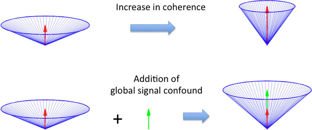
Simplified geometric model of resting-state data and the global signal. In the top row, an increase in the coherence of the resting-state vectors (blue lines) leads to both an increase in the magnitude of the global mean signal (red arrows) and a decrease in the angle between the vectors and the global signal. In the bottom row, the addition of a global signal confound (green arrow) leads to both an increase in the magnitude of the global mean signal and a decrease in the angle between the vectors and the global signal. Note, however, that in the top row the length of the resting-state vectors remains constant, while in the bottom row the additive signal confound causes the vectors to increase in length. As the additive confound grows in magnitude, the vectors become more correlated, obscuring the true underlying correlation.

On the other hand, the angular spread of the vectors can also be modified through the addition of a global signal confound, shown as the green arrow in the bottom row of Figure 3. This additive global signal confound will have three effects: (1) an increase in the global signal vector (sum of the red and green arrows); (2) an increase in the lengths of the individual vectors; and (3) a reduction in the angle between the individual vectors and the global signal (from 60 degrees to 42 degrees), with a corresponding increase in the correlation between the vectors.

The simplified model of Figure 3 shows that a change in the angular spread of the resting-state vectors can reflect two very different scenarios. Furthermore, it is possible to distinguish between the two scenarios by examining the lengths of the individual vectors. If the angular spread decreases without a concomitant increase in the length of the vectors, we can attribute the change in angular spread and the accompanying change in global mean vector to a “true” increase in the coherence of the vectors. On the other hand, if the decrease in angular spread is associated with an increase in the length of the individual vectors, then it is more likely that the changes in angular spread and global mean vector are due to the presence of an additive global signal confound.

The simplified model also suggests that the measured global signal can be viewed as the sum of two components: (a) a desired component (red arrow) which reflects the inherent correlation of the resting-state vectors and (b) a nuisance component (green) arrow reflecting an additive signal. Global signal regression removes both components, whereas the ideal global signal correction method would remove only the nuisance component while preserving the desired component.

Application of Geometric View towards Global Signal Correction

To determine whether the experimental data supports the existence of an additive global signal confound, we can consider the relationship between the median angle and the mean BOLD signal amplitude, where the latter metric is calculated by taking the average of the lengths of all the BOLD time series vectors in the un-normalized data matrix ϒ (see also Methods section). Based on our simplified model, if an additive signal confound is present, we expect to find an inverse relation between the median angle and the mean BOLD signal amplitude as measured across different datasets. In addition, we expect to find a positive correlation between the mean BOLD signal magnitude and the magnitude of the mean global signal vector. As shown in Figure 6 of the Results section, these relations appear very clearly in the experimental data, supporting the presence of an additive global signal confound and justifying the application of some form of global signal correction.

Figure 6.

The median angle exhibits an inverse relation with both mean BOLD amplitude (panel a) and global signal amplitude (panel c). The vertical dashed line in panel a indicates the minimum mean BOLD amplitude, while the horizontal dashed line indicates the linear fit median angle value corresponding to this amplitude. A vector plot (panel c) based on the median angle and mean BOLD amplitudes emphasizes that the length of the vector increases as the median angle decreases. The mean BOLD amplitude and global signal amplitude are strongly correlated as shown in panel d.

As discussed above, an ideal global correction method would remove only the additive global signal confound while preserving the desired component that exists due to the presence of correlations in the brain. In practice, we will not be able to uniquely identify the additive confound from the measured data alone. However, as an initial step, we can consider using the inverse relation between median angle and mean BOLD magnitude to correct for differences in the additive confound. First, we note that resting-state data sets with high median angles and low mean BOLD magnitudes are likely to be the least contaminated by an additive global confound. Indeed, datasets with high median angles have correlation maps with anti-correlations between the default mode network and the task positive network that are typically seen only after the application of global signal regression (e.g. Figures 2d and top row of Figure 7, subject A, with median angles of 62 and 58 degrees, respectively). Second, we observe that increasing the median angle of a dataset to match that of a “target” dataset with high median angle will act to diminish the contribution of an additive signal confound. For example, we may view the idealized dataset in the lower lefthand corner of Figure 3 as the target dataset. If we increase the angle of the dataset in the lower righthand corner to match that of the target dataset, this process will effectively remove the contribution of the additive confound (i.e. the green arrow).

Figure 7.

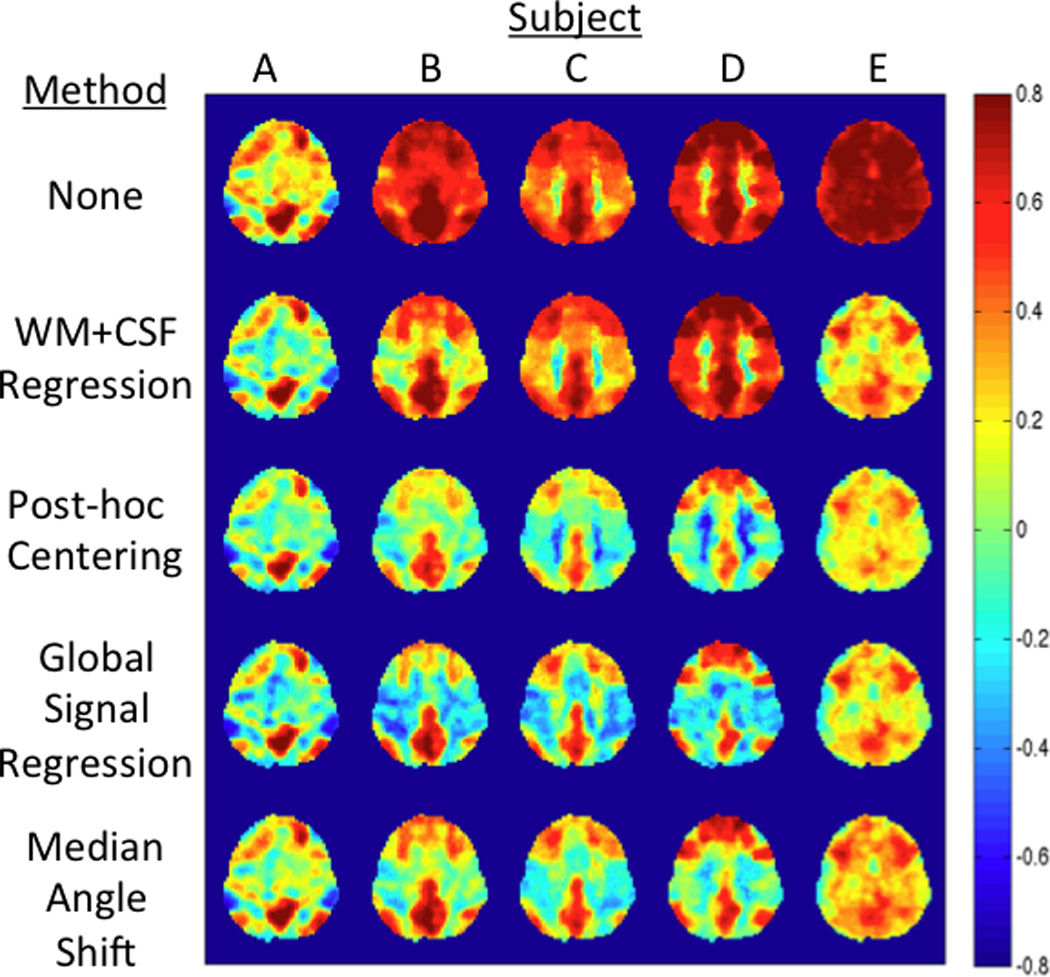
Comparison of different global signal correction methods. The correlation maps in the top row are obtained after standard preprocessing steps (i.e. removal of low frequency terms and motion regressors). The median angles are 58, 39, 37, 38, and 30 degrees for subjects A through E, respectively.

METHODS

Subjects and data acquisition

The data used in this paper were originally analyzed by (Fox et al., 2007) and downloaded from www.brainscape.org (dataset BS002). These data were acquired from 17 normal right-handed young adults (9 females) on a 3T Siemens Allegra MR scanner. All subjects underwent four BOLD-EPI fixation runs (32 slices, TR = 2.16 s, TE = 25 ms, 4×4×4 mm), each lasting 7 minutes (194 frames). During these scans, subjects were instructed to look at a crosshair, and to remain still and awake. High-resolution T1-weighted anatomical images were also acquired for the purpose of anatomical registration (TR = 2.1 s, TE = 3.93 ms, flip angle = 7°, 1×1×1.25 mm).

Data preprocessing

A series of common image preprocessing steps was conducted with the AFNI software package (Cox, 1996). The first 9 frames from each run were discarded to minimize longitudinal relaxation effects. All BOLD-fMRI images were slice-timing corrected to account for interleaved acquisition and coregistered for head-motion correction. The resultant EPI images were converted to stereotaxic coordinates of Talairach and Tournoux, resampled to 3-mm cubic voxels, and then spatially smoothed using a 6-mm full-width-at-half-maximum isotropic Gaussian kernel. Nuisance terms were removed from each voxel’s time course using multiple linear regression. These were: (1) a constant term to model the temporal mean of each voxel, (2) a linear trend, and (3) six motion parameters obtained from the head motion correction algorithm. A temporal low pass filter was applied to the remaining time course using a cutoff frequency of 0.1 Hz (Cordes et al., 2000; Yan et al., 2009).

Decomposition of data

The pre-processed data were normalized to be unit-norm and then decomposed using a singular value decomposition (SVD). The correlation map with a seed region in the posterior cingulate cortex (see below for ROI definition) was expanded as the weighted sum of component correlation maps as described in Equation 3. Note that instead of the original order of the singular values, components are ordered using the modified ranking scheme described in the Theory section. Low-dimensional approximations to the correlation map were obtained by truncating the weighted sum.

Calculation of Metrics

For each voxel time series (prior to normalization to unit norm for the SVD), a percent change time series was obtained by subtracting the mean value and then dividing the resulting difference by the mean value. A global mean signal was formed as the average of the percent change time series across all voxels within the brain, and the standard deviation of the global signal was recorded for each run. For each voxel, we also computed the standard deviation of the percent change time series and defined the mean BOLD signal amplitude for each run as the average of the standard deviation values across the brain. To compute the median angle, we obtained the projection of each voxel time series (normalized to unit norm) onto the first principal component obtained from the SVD described above and calculated the corresponding angle as the inverse cosine of the projection value. We then recorded the median of these angles across the entire brain for each run.

Correlation Maps

A seed region in the posterior cingulate cortex was defined using a sphere with radius of 6-mm (2 voxels) centered about point [0,−52,26] in Tailarach space. The coordinates were obtained by converting the MNI coordinates in a previous paper (Van Dijk et al., 2010) to Tailarach coordinates using a nonlinear MNI to Talairach conversion algorithm (Lacadie et al., 2008). A seed signal was formed as the average time course of voxels within the PCC region. A correlation map was then computed by correlating the seed signal with the time-course from every voxel in the brain.

In addition to the standard correlation map, we also formed correlation maps after (1) removal of white matter and cerebral spinal fluid (CSF) regressors; (2) post-hoc centering of the correlation values; (3) global signal regression; and (4) the proposed median angle shift correction method (defined below). For white matter and CSF regression, we projected out the average signals from white matter and CSF regions prior to computing the correlation map. For post-hoc centering of the data, we converted correlation values from the standard correlation map to z-scores, centered the z-scores about zero, and then converted the centered z-scores back to correlation values (Lowe et al., 1998). To implement global signal regression, we projected out the global mean signal from all voxel time series prior to the computation of the correlation map.

As a preliminary test of the proposed median shift correction method, we computed the least squares fit of the median angles to the mean BOLD magnitude and defined the target median angle as the fit value (θ_TARGET = 66 degrees; indicated by the black horizontal dashed line in Figure 6a) corresponding to the minimum observed mean BOLD magnitude in the sample (indicated by black vertical dashed line in Figure 6a). We used the linear fit value as the target angle instead of the maximum observed angle, so as to reduce the effects of data variance on the selection of the angle. For each resting-state data set, we then computed the difference Δθ = θ_TARGET − θ_SCAN between the target median angle and the observed median angle. If the difference was positive, we increased the angle between the first principal component and all resting-state vectors in the data set by the value Δθ. In other words, for Δθ > 0, the angle of each vector after the median angle shift was θ̃_i = θ_i + Δθ, where θ_i denotes the original angle between the ith resting-state vector and the first principal component. For Δθ ≤ 0 (i.e. data points above the black horizontal line in Figure 6a), no shift was applied to the dataset.

RESULTS

Decomposition of correlation maps

To demonstrate the decomposition of a correlation map, Figure 1a shows a full (i.e. using all components) correlation map obtained using a seed signal from the PCC region with maps of the top 3 correlation components shown in Figures 1c through 1e, i.e. $\frac{1}{\Vert {\overline{\mathbf{y}}}_s\Vert }{\sigma }_{i(k)}^2{\overline{v}}_{i(k),j}{\mathbf{v}}_{i(k)}$ for k ranging from 1 to 3 with the modified ranking scheme. (As there was space in the plot, the 4^th component is also shown.) The correlation map associated with the first component (PC1) represents the correlation with the component that is similar to the global signal. A low dimensional approximation to the full correlation map using the sum of the top 3 components is shown in Figure 1b (obtained using Equation 3 with K = 3). It exhibits a high degree of similarity to the full correlation map in Figure 1a. Supplementary Figure 1 provides additional examples of the decomposition for a representative slice and run from each subject

Figure 1.

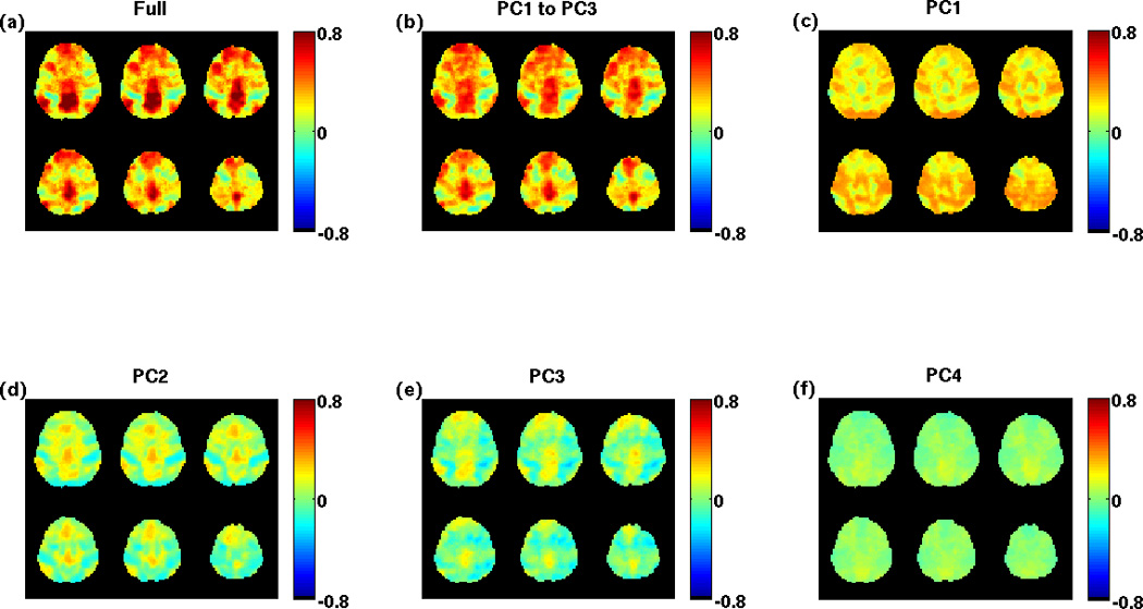
A correlation map using a seed signal from the PCC is shown in panel (a). The low-dimensional approximation using the sum of the top 3 ranked component maps is shown in panel (b). The individual component correlation maps are shown in panels (c) through (f).

To quantify the extent to which the low dimensional approximations can represent the full correlation maps, we computed the ratio of the energy of the low dimensional approximation using the top K components to the energy of the full correlation map which uses all M components (see also text prior to Equation 3). Using the notation of the Theory section, this ratio can be written as $\left({\displaystyle \sum _{k=1}^K}{\left({\sigma }_{i(k)}^2{\overline{v}}_{i(k),j}\right)}^2/{\displaystyle \sum _{k=1}^M}{\left({\sigma }_{i(k)}^2{\overline{v}}_{i(k),j}\right)}^2\right)$. Figure 4a plots the ratio (denoted as relative energy) for low dimensional approximations using from 1 to 20 components, where the maps were computed using a PCC seed signal and the mean, minimum, and standard deviations across the sample are shown. Only a few components are needed to account for a significant portion of the norm of the full correlation map. For example, low-dimensional approximations using the top 3 components account for 95.0 ± 4.1% of the total energy, with a minimum of value across all subjects and runs of 82.5%. For comparison, for the conventional ranking system based on singular values (with relative energy curves shown in Figure 4b), the top 3 components account for 91.9 ± 7.5% of the total energy with a minimum value of 70.4%. As an example of the difference between the ranking schemes, Supplementary Figure 2 compares correlation maps decomposed with the modified (top section) and conventional (bottom section) ranking schemes for a representative subject and run. The approximation using the top 3 components according to the modified ranking scheme clearly provides a better representation than that obtained with the conventional ranking scheme.

Figure 4.

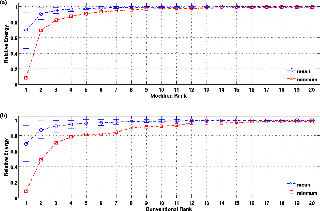
Ratio of the energy of the low-dimensional approximation to the energy of the full correlation map plotted against the number of components in the approximation. Data are displayed as mean +/− standard deviation.

Low-dimensional View of the Data

Since the structure of the correlation maps is well captured by the top 3 components, it is helpful to view the data in the low-dimensional space spanned by these components. In the top row of Figure 2, we present three-dimensional views of the data in the space defined by the top 3 ranked components for three representative datasets. The colors on the sphere indicate the number of voxels lying within each sector of the sphere and the axes are labeled by the rank of the principal component. The median angles are 62, 40, and 30 degrees for panels (a) through (c), respectively. The bottom row of Figure 2 shows the corresponding correlation maps obtained with a seed signal from the PCC. As the angular spread of the resting-state vectors decreases, there is a widespread increase in correlation values across the map.

Similarity of the global signal and the first principal component

We found that the first principal component was highly correlated with the global signal. In Figure 5a, we show nearly perfect agreement between the first principal component (blue) and global signal (red) from a representative dataset. For the entire sample, the correlation coefficients between the first principal component and the global signal are shown in Figure 5b, with the bar indicating standard deviation over runs for each subject. The correlation values are all above 0.94 (with corresponding p < 10⁻⁶). As shown in the appendix, this relation between the first principal component and the global signal is expected whenever the projections of the data onto the global signal are predominantly positive. Across the 68 datasets examined, the average percentage of positive projections is 99.0% ± 0.69%. In prior work, (Andersson et al., 2001) have suggested that the presence of primarily positive projections is one of the expected characteristics of a global signal.

Figure 5.

The relationship between the global mean signal and PC1. (a) The first principal component (in blue) is almost identical to the global mean signal (in red) for a representative dataset. (b) The correlation values between these two terms are significant for all subjects and runs (p < 10⁻⁶).

Relation between Median Angle and Mean BOLD Amplitude

Figure 6a shows that there is a significant inverse correlation (r = −0.78, p < 10⁻⁶) between median angle and the mean BOLD amplitude. As discussed in the Theory section, this inverse correlation is consistent with the presence of an additive global confound. As each point in Figure 6a is characterized by an amplitude and a median angle, we can replot each point with the y-coordinate given by the amplitude multiplied by the cosine of the median angle (corresponding to the projection of the data onto the first principal component) and the x-coordinate given by the amplitude multiplied by the sine of the median angle (corresponding to the projection of the data onto the orthogonal complement of the first principal component). The results of this procedure are shown in Figure 6b. In a similar fashion, we have replotted the linear fit to the data (red line) in Figure 6a as the red line in Figure 6b. Arrows are used to indicate several representative points on the linear fit. Viewing these as vectors, we can see that the lengths of these vectors increases as their angles decrease, consistent with the simplified model shown in Figure 3.

It is interesting to note that the linear fit to the data (solid red line) indicates that when the mean BOLD amplitude goes to zero the median angle will be 86 degrees. Note that effect of global signal regression is to remove the part of the signal that is parallel to the global mean component. Due to the similarity between the first principal component and the global mean, global signal regression results in residual vectors that are at an angle of 90 degrees to the first principal component. As the experimental data indicate that a median angle of 86 degrees is a fairly strict upper bound, global signal regression is likely to be too aggressive in removing the signal component that is parallel to the global mean signal.

In Figures 6c and 6d, we find a significant inverse correlation (r = −0.92; p < 10⁻⁶) between the median angle and the global signal amplitude and a significant positive correlation (r = 0.93; p < 10⁻⁶) between the mean BOLD amplitude and the magnitude of the global signal, respectively. These observations are consistent with the predictions of the simplified model shown in Figure 3 and further support the existence of an additive confound.

Comparison of Global Signal Correction Approaches

In Figure 7, we provide a qualitative comparison of the various global signal correction approaches using 5 representative datasets (labeled A through E) with median angles of 58, 39, 37, 38, and 30 degrees, respectively. The uncorrected correlation maps are shown in the top row, with corrected correlation maps obtained using white matter and CSF regression, post-hoc centering, global signal regression, and the proposed median angle shift approach shown in the successive rows. For the dataset (Subject A) with a relatively large median angle of 58 degrees, the maps obtained with all the methods are exhibit similar patterns. However, for subjects B through C, the white matter and CSF regression method does not perform well in revealing the underlying regional correlations, consistent with the findings of (Fox et al., 2009). For subjects C and D, the post-hoc centering method results in anti-correlations between the PCC and white matter, that are likely to be spurious and similar to artifacts reported by (Fox et al., 2009). Global signal regression and the median angle shift method give similar maps across all subjects, with the main difference being that the number of large negative correlations is noticeably smaller in the median angle shift maps. Additional comparisons of the various correction methods are shown in Supplementary Figures 3 through 7 for correlation maps obtained using seed regions in the intraparietal sulcus (part of the dorsal attention network), the ventral frontal cortex (part of the ventral attention network), the visual cortex, the auditory cortex, and the motor cortex, respectively. The performance with these maps is similar to what was observed for the maps in Figure 7.

The difference in the number of negative correlations produced with the various approaches can also be seen in the correlation coefficient histograms shown in Figure 8. Whereas the post-hoc centering and global signal regression approaches result in distributions that are roughly centered about zero correlation, the median angle shift approach generates distributions with a positive mean. Across the sample of 68 datasets, the averages (± standard deviation) of the mean values of the correlation coefficient distributions were 0.001± 0.022 and 0.149±0.047 for global signal regression and the median angle shift approach, respectively. The similarities and differences between the various correction methods are further addressed in the Discussion section.

Figure 8.

Comparison of correlation coefficient distributions for 5 representative subjects obtained using different global signal correction methods.

DISCUSSION

We have shown that the global signal in resting-state fMRI can be viewed as the sum of two components: a component that reflects the inter-regional correlations between resting-state vectors and an additive global signal confound component. An ideal global signal correction method would remove the additive signal confound while preserving the desired component. For data from a single experimental run, it is not possible in general to distinguish the two components without additional information, such as external physiological measurements. However, an examination of data across multiple subjects and experimental runs can provide insight into the relative contributions of the two components. In particular, we have shown that the observed inverse relationship between median angle and mean BOLD amplitude is consistent with the presence of an additive confound. Making use of this observation, we proposed a global signal correction approach in which the angular distributions of datasets with small median angles were shifted to attain a larger target median angle. In a preliminary demonstration, the median angle shift approach appears to effectively minimize the effects of the global signal confound.

While the results presented in this paper support the presence of an additive global signal confound, they do not provide information about the relative contributions of neuronal and physiological (e.g. respiratory and cardiac activity) sources to the additive confound. Prior work has shown that physiological sources contribute to the overall global signal (Chang and Glover, 2009) and that these sources can be reasonably considered to be components of the additive confound. However, physiological sources do not account for all of the variance observed in the global signal, suggesting the presence of neural components. Indeed, a recent study using simultaneous electrophysiological and fMRI measures in primate models provides evidence of neural contributions to widespread global fMRI activity (Schölvinck et al., 2010). Although at first glance it would seem prudent to avoid removing any component of the global signal that can be explained by neural sources, a deeper consideration of the issue suggests that the neural global contribution can be parsed into a desired component that is of interest and an additive confound component. Referring to the schematic diagram of Figure 3, a neural contribution that increases the magnitude of the BOLD resting-state vectors while reducing their angular spread can be considered an additive confound. In contrast, a neural contribution that reduces the angular spread but does not increase the magnitude of the BOLD resting-state vectors most likely reflects the increased coherence of the neural fluctuations in different brain regions and would not be considered a confound. Future studies with both physiological measures and simultaneous acquisition of EEG and fMRI measures could help to elucidate the extent to which global fluctuations of a neural origin can be considered an additive confound.

In comparing the proposed median angle shift approach to global signal regression, we note that both methods reduce the component of the resting-state signal that is parallel to the global mean signal. The main difference between the two approaches is the extent to which this component is reduced. Global signal regression completely eliminates this component, and therefore forces the existence of negative correlations. In addition, global signal regression does not make a distinction between the component of the global mean signal that exists whenever there is mutual correlation between resting-state vectors and the nuisance component that can be attributed to an additive confound. In contrast, the median angle shift approach aims to reduce the component that is consistent with the presence of an additive confound, while largely preserving the component that reflects inherent correlations. Due to the reduction of the additive confound component, the median angle shift method will shift the mean of the distribution of correlation coefficients towards zero (e.g. Figure 8), but to a smaller extent than global signal regression. Thus, the number of negative correlations observed after application of the method will generally be less than that observed with global signal regression.

As the median angle shift approach results in a shift of the correlation values, it appears initially to share some similarities with post-hoc centering of the correlation values. However, there are some important differences. First, post-hoc centering centers the z-scores of the correlation values about zero. As compared to the median angle shift approach, which does not impose a requirement of a symmetric distribution of correlation values, the post-hoc centering method leads to a greater shift and a greater number of negative correlation values. Second, post-hoc centering is typically applied to the correlation values obtained using a specific seed region, and the process must therefore be repeated for each seed region. In contrast, the median angle shift approach is applied directly to the resting-state data and may therefore be considered a pre-processing step (similar to global signal regression) that is applied prior to the computation of correlation maps.

Although the preliminary performance of the median angle shift approach appears promising, further work is required to improve the method and validate its broader efficacy. For example, we used the minimum mean BOLD amplitude observed over the sample to determine the target angle. This choice was based on the observation that the correlation maps from datasets with small mean BOLD amplitudes exhibited minimal contamination from global signal confounds. However, this method of determining the target angle would not work well for samples in which all the datasets exhibited the presence of a strong additive global signal component, and alternate approaches would need to be developed to address this type of situation. In our initial implementation, we applied a constant shift angle Δθ to all resting-state vectors within a dataset. This may not be optimal for resting-state vectors that are already nearly orthogonal to the global signal, as these vectors most likely contain minimal contributions from the additive confound. Adaptive schemes in which the shift angle is a function of the vector angle could provide better performance and would be useful to consider in future studies. Finally, the median angle shift approach should be viewed as an initial attempt to make use of the geometric framework to reduce global signal confounds, and it is likely that future efforts utilizing the framework will result in alternate approaches that provide better performance.

Recently, (Hampson et al., 2010) have proposed an alternate global signal correction approach in which a mean connectivity z-score is used as a covariate in the analysis of connectivity measures across a sample. Similar to post-hoc centering, the proposed approach relies on the specification of a seed region to define the mean connectivity. Hampson and colleagues found that their approach improves the strength of the relation between connectivity measures and behavioral metrics without altering the distribution of the connectivity measures. It would be useful to determine whether the median angle shift approach offers similar gains in performance. In addition, this experimental approach can be used to compare the performance of the median angle shift method with other methods, such as global signal regression and post-hoc centering.

We found that low-dimensional views (e.g. Figure 2) were helpful for developing intuition regarding the geometry of resting-state data. To form these views, we used a modified ranking scheme for ordering the principal components. While the modified ranking scheme is not strictly required for generating the low dimensional views, its improved performance in decomposing correlation maps (e.g. Supplementary Figure 2) facilitates a better understanding of the relation between correlation maps and the low-dimensional views (He and Liu, 2011). Another potential application of the principal component decomposition and modified ranking scheme is the denoising of seed-based correlation maps to help improve measures of connectivity. This could be accomplished by retaining only those components that best approximate each correlation map, with a seed-dependent selection of the components based on the modified ranking scheme. Further work would be needed to evaluate the efficacy of this denoising approach for the analysis of resting-state fMRI studies. Finally, although the principal component decomposition played a critical role in our development of the geometric picture of the resting state data, the full decomposition is not required for the implementation of the median angle shift method, which requires only the computation of the angle between each voxel’s time series vector and the global mean signal.

In conclusion, we have presented an analysis of resting-state data that supports the presence of an additive global confound. For correlation-based analysis of resting-state data, it is desirable to minimize the effects of this additive confound. We have outlined an initial approach for reducing the effects of the additive confound and described areas that would benefit from further investigation.

Highlights.

Research highlights for

A Geometric View of Global Signal Confounds in Resting-State Functional MRI

• Geometric view of effect of additive global signal confounds.

• Method for reducing effect of additive confounds.

• Comparison with other global signal correction approaches.

Supplementary Material

01

A correlation map using a seed signal from the PCC is shown in the top row for a representative run and slice from each of the 17 subjects. The low-dimensional approximations using the sum of the top 3 ranked component maps are shown in the second row, with the individual component maps shown in the third to fifth rows.

02

Correlation maps decomposed with the modified (top section) and conventional (bottom section) ranking schemes for a representative subject and run.

03

Comparison of different global signal correction methods for correlation maps showing the dorsal attention network and obtained using a seed region in the right intraparietal sulcus (Tailarach coordinates [27,−58,49]). Coordinates from (Fox et al., 2006).

04

Comparison of different global signal correction methods for correlation maps showing the ventral attention network and obtained using a seed region in the right ventral frontal cortex (Tailarach coordinates [37,18,1]). Coordinates from (Fox et al., 2006).

05

Comparison of different global signal correction methods for correlation maps obtained using a seed region in the visual cortex ( Tailarach coordinates [28,−80,2]). Coordinates from (Van Dijk et al., 2010)

06

Comparison of different global signal correction methods for correlation maps obtained using a seed voxel in the auditory cortex (Tailarach coordinates ([41,−25,8]). Coordinates from (Van Dijk et al., 2010)

07

Comparison of different global signal correction methods for correlation maps obtained using a seed region in the motor cortex (Tailarach coordinates ([32,−22,53]). Coordinates from (Van Dijk et al., 2010)

Appendix

A1 Principal Components Decomposition of Correlation Map

Using the SVD notation Y = UΣV^T presented in the Theory section, the eigen-decomposition of the correlation coefficient matrix is C = Y^TY = VΣ²V^T, where the columns of V are the spatial principal components (also referred to as eigen-images). It is useful to write the correlation coefficient matrix in expanded form as the sum of outer products of the eigen-images

$$\mathbf{C}=\mathbf{V}{\mathrm{\Sigma }}^2{\mathbf{V}}^T={\mathrm{\sigma }}_1^2{\mathbf{v}}_1{\mathbf{v}}_1^T+{\mathrm{\sigma }}_2^2{\mathbf{v}}_2{\mathbf{v}}_2^T+\cdots +{\mathrm{\sigma }}_M^2{\mathbf{v}}_M{\mathbf{v}}_M^T={\displaystyle \sum _{i=1}^M}{\mathrm{\sigma }}_i^2{\mathbf{v}}_i{\mathbf{v}}_i^T$$ (A1)

where v_i is the ith spatial principal component. Note that the matrix C contains the pair-wise correlations between all pairs of voxel time-courses. If we are interested in the correlation map obtained with one of the voxels as the seed voxel, we can choose either a single row or column. For example, the jth column of C contains the correlations of all voxels with the jth voxel. This correlation map may be expressed as

$${\mathbf{c}}_j={\displaystyle \sum _{i=1}^M}{\mathrm{\sigma }}_i^2{v}_{i,j}{\mathbf{v}}_i$$ (A2)

where v_i,j represents the jth element of the ith component vector.

Equation A2 applies in the case when we are considering pair-wise correlations between the time-courses from single voxels. A common practice is to compute the seed time-course as the average of the time-courses from a region of interest (ROI), such as a spherical region within the posterior cingulate cortex (PCC). When using an average seed time-course, the correlation map is simply the average of the correlation maps obtained with using the seed voxels in the ROI and normalized by the norm of the average seed signal. The correlation map with a seed region spatially centered about the jth voxel can be written as

$${\mathbf{C}}_j=\frac{1}{\Vert {\overline{\mathbf{y}}}_s\Vert }{\displaystyle \sum _{i=1}^M}{\mathrm{\sigma }}_i^2{\overline{v}}_{i,j}{\mathbf{v}}_i$$ (A5)

where ‖y_S‖ is norm of the average seed signal and ${\overline{v}}_{i,j}=\frac{1}{L}{\displaystyle \sum _{l\in J}}{v}_{i,l}$ is the mean of the component factors, with J denoting the set of the L voxel indices for the ROI.

A2 Relation between the global signal and the first principal component

To gain insight into the relation between the first principal component and the global signal, we first note that the temporal principal components of the data matrix are the left singular vectors u_i (i.e. the columns of U). These are also the eigenvectors of the matrix product YY^T. The global signal is defined as the mean ȳ of the column vectors of the data matrix Y. In the results section, we observed empirically that the projections of the data onto global signal were predominantly positive. In this section, we want to show that when this condition holds, the global signal ȳ is an approximate eigenvector of the matrix product YY^T and has the largest associated eigenvalue.

We first write the data matrix as Y = Y̅ + Ỹ where the projection of the data onto the global signal is denoted as Y̅ = PY with P = ȳ(ȳ^T ȳ)⁻¹ȳ^T defined as the projection matrix for the global signal. The residual data matrix is defined as Ỹ = (I − P)Y where I is the identity matrix. With this notation the matrix product becomes ${\mathbf{\text{YY}}}^T={\overline{\mathbf{\text{YY}}}}^T+\tilde{\mathbf{Y}}{\tilde{\mathbf{Y}}}^T+\overline{\mathbf{Y}}{\tilde{\mathbf{Y}}}^T+\tilde{\mathbf{Y}}{\overline{\mathbf{Y}}}^T$. Multiplying this by the global signal ȳ and taking into account the orthogonality between ȳ and the columns of Ỹ, we obtain YY^Tȳ = (Y̅ + Ỹ)Y̅^Tȳ. Without loss of generality, we may normalize ȳ to have unit norm. We next note that Ȳ = ȳc^T where c^T = ȳ^TY is a 1 × N vector whose ith element is the cosine of the angle θ_i between the ith normalized data vector and the normalized global signal. Using this notation, we derive the following expression YY^Tȳ = c^Tcȳ + Ỹc.

Now we consider the relative magnitudes of the terms c^Tcȳ and Ỹc when the projections of the data onto the global signal are one-sided. A specific case of this assumption occurs when the angles θ_i are uniformly distributed over the interval −π/2 to π/2. In this case, the expected magnitude of c^Tcȳ is N /2. To estimate the expected value of Ỹc, we first note that the sum of the columns of Ỹ is zero (i.e. Ỹ1_N = 0 where 1_N is a column vector of 1’s). This relation can be readily derived from the definitions of the projection matrix and the fact that $\overline{\mathbf{y}}=\frac{1}{N}\mathbf{Y}{\mathbf{1}}_N$ (prior to normalization). The geometric interpretation is that the residual vectors (i.e. columns of Ỹ) tend to be uniformly distributed around the global signal vector. For the term Ỹc, we are taking the sum of the residual columns weighted by the cosine of the angle between the data and the global signal. For each angle, the uniform distribution of residual vectors will also tend to cause a cancellation in the vector sum, such that the magnitude of the term Ỹc will be small compared to the amplitude of c^Tcȳ and therefore YY^Tȳ ≈ c^Tcȳ. Thus, v₁ ≈ ȳ is an approximate eigenvector of YY^T with an eigenvalue of approximately N/2. The eigenvalues of YY^T are positive and their sum is equal to N, which is also the trace of the matrix. Thus, the sum of all eigenvalues excluding the one associated with v₁ is approximately N /2. In general, this sum is split among more than one eigenvalue, so that the magnitude of any given eignvalues is less than N /2. Thus, v₁ will tend to be the dominant eigenvector with the largest associated eigenvalue.

References

- Allen G, Barnard H, McColl R, Hester AL, Fields JA, Weiner MF, Ringe WK, Lipton AM, Brooker M, McDonald E, Rubin CD, Cullum CM. Reduced hippocampal functional connectivity in Alzheimer disease. Arch Neurol. 2007;64:1482–1487. doi: 10.1001/archneur.64.10.1482. [DOI] [PubMed] [Google Scholar]
- Andersson JL, Ashburner J, Friston K. A global estimator unbiased by local changes. NeuroImage. 2001;13:1193–1206. doi: 10.1006/nimg.2001.0763. [DOI] [PubMed] [Google Scholar]
- Birn RM, Diamond JB, Smith MA, Bandettini PA. Separating respiratory-variation-related fluctuations from neuronal-activity-related fluctuations in fMRI. NeuroImage. 2006;31:1536–1548. doi: 10.1016/j.neuroimage.2006.02.048. [DOI] [PubMed] [Google Scholar]
- Chang C, Glover GH. Effects of model-based physiological noise correction on default mode network anti-correlations and correlations. NeuroImage. 2009;47:1448–1459. doi: 10.1016/j.neuroimage.2009.05.012. [DOI] [PMC free article] [PubMed] [Google Scholar]
- Cordes D, Haughton VM, Arfanakis K, Wendt GJ, Turski PA, Moritz CH, Quigley MA, Meyerand ME. Mapping functionally related regions of brain with functional connectivity MR imaging. AJNR Am J Neuroradiol. 2000;21:1636–1644. [PMC free article] [PubMed] [Google Scholar]
- Cox RW. AFNI-software for analysis and visualization of functional magnetic resonance neuroimages. Comput. Biomed. Res. 1996;29:162–173. doi: 10.1006/cbmr.1996.0014. [DOI] [PubMed] [Google Scholar]
- Fox MD, Corbetta M, Snyder AZ, Vincent JL, Raichle ME. Spontaneous neuronal activity distinguishes human dorsal and ventral attention systems. Proc Natl Acad Sci U S A. 2006;103:10046–10051. doi: 10.1073/pnas.0604187103. [DOI] [PMC free article] [PubMed] [Google Scholar]
- Fox MD, Snyder AZ, Vincent JL, Raichle ME. Intrinsic fluctuations within cortical systems account for intertrial variability in human behavior. Neuron. 2007;56:171–184. doi: 10.1016/j.neuron.2007.08.023. [DOI] [PubMed] [Google Scholar]
- Fox MD, Zhang D, Snyder AZ, Raichle ME. The global signal and observed anticorrelated resting state brain networks. J Neurophysiol. 2009;101:3270–3283. doi: 10.1152/jn.90777.2008. [DOI] [PMC free article] [PubMed] [Google Scholar]
- Friston KJ, Frith CD, Fletcher P, Liddle PF, Frackowiak RS. Functional topography: multidimensional scaling and functional connectivity in the brain. Cereb Cortex. 1996;6:156–164. doi: 10.1093/cercor/6.2.156. [DOI] [PubMed] [Google Scholar]
- Friston KJ, Frith CD, Liddle PF, Frackowiak RS. Functional connectivity: the principal-component analysis of large (PET) data sets. J Cereb Blood Flow Metab. 1993;13:5–14. doi: 10.1038/jcbfm.1993.4. [DOI] [PubMed] [Google Scholar]
- Hampson M, Driesen N, Roth JK, Gore JC, Constable RT. Functional connectivity between task-positive and task-negative brain areas and its relation to working memory performance. Magnetic Resonance Imaging. 2010;28:1051–1057. doi: 10.1016/j.mri.2010.03.021. [DOI] [PMC free article] [PubMed] [Google Scholar]
- Hampson M, Driesen NR, Skudlarski P, Gore JC, Constable RT. Brain connectivity related to working memory performance. J Neurosci. 2006;26:13338–13343. doi: 10.1523/JNEUROSCI.3408-06.2006. [DOI] [PMC free article] [PubMed] [Google Scholar]
- He H, Liu TT. Principal Components Analysis Reveals the Correlation Structure of Resting-State fMRI Data. 10th Annual Meeting of the International Society for Magnetic Resonance in Medicine; Montreal. 2011. p. 1607. [Google Scholar]
- Lacadie CM, Fulbright RK, Rajeevan N, Constable RT, Papademetris X. More accurate Talairach coordinates for neuroimaging using non-linear registration. NeuroImage. 2008;42:717–725. doi: 10.1016/j.neuroimage.2008.04.240. [DOI] [PMC free article] [PubMed] [Google Scholar]
- Lowe MJ, Mock BJ, Sorenson JA. Functional connectivity in single and multislice echoplanar imaging using resting-state fluctuations. NeuroImage. 1998;7:119–132. doi: 10.1006/nimg.1997.0315. [DOI] [PubMed] [Google Scholar]
- Murphy K, Birn RM, Handwerker DA, Jones TB, Bandettini PA. The impact of global signal regression on resting state correlations: are anti-correlated networks introduced? NeuroImage. 2009;44:893–905. doi: 10.1016/j.neuroimage.2008.09.036. [DOI] [PMC free article] [PubMed] [Google Scholar]
- Schölvinck ML, Maier A, Ye FQ, Duyn JH, Leopold DA. Neural basis of global resting-state fMRI activity. Proc Natl Acad Sci USA. 2010;107:10238–10243. doi: 10.1073/pnas.0913110107. [DOI] [PMC free article] [PubMed] [Google Scholar]
- Van Dijk KRA, Hedden T, Venkataraman A, Evans KC, Lazar SW, Buckner RL. Intrinsic functional connectivity as a tool for human connectomics: theory, properties, and optimization. J Neurophysiol. 2010;103:297–321. doi: 10.1152/jn.00783.2009. [DOI] [PMC free article] [PubMed] [Google Scholar]
- Weissenbacher A, Kasess C, Gerstl F, Lanzenberger R, Moser E, Windischberger C. Correlations and anticorrelations in resting-state functional connectivity MRI: a quantitative comparison of preprocessing strategies. NeuroImage. 2009;47:1408–1416. doi: 10.1016/j.neuroimage.2009.05.005. [DOI] [PubMed] [Google Scholar]
- Yan L, Zhuo Y, Ye Y, Xie SX, An J, Aguirre GK, Wang J. Physiological origin of low-frequency drift in blood oxygen level dependent (BOLD) functional magnetic resonance imaging (fMRI) Magnetic Resonance in Medicine. 2009;61:819–827. doi: 10.1002/mrm.21902. [DOI] [PubMed] [Google Scholar]
Associated Data
This section collects any data citations, data availability statements, or supplementary materials included in this article.
Supplementary Materials