Abstract
Purpose: Prior image constrained compressed sensing (PICCS) is an image reconstruction framework which incorporates an often available prior image into the compressed sensing objective function. The images are reconstructed using an optimization procedure. In this paper, several alternative unconstrained minimization methods are used to implement PICCS. The purpose is to study and compare the performance of each implementation, as well as to evaluate the performance of the PICCS objective function with respect to image quality.
Methods: Six different minimization methods are investigated with respect to convergence speed and reconstruction accuracy. These minimization methods include the steepest descent (SD) method and the conjugate gradient (CG) method. These algorithms require a line search to be performed. Thus, for each minimization algorithm, two line searching algorithms are evaluated: a backtracking (BT) line search and a fast Newton-Raphson (NR) line search. The relative root mean square error is used to evaluate the reconstruction accuracy. The algorithm that offers the best convergence speed is used to study the performance of PICCS with respect to the prior image parameter α and the data consistency parameter λ. PICCS is studied in terms of reconstruction accuracy, low-contrast spatial resolution, and noise characteristics. A numerical phantom was simulated and an animal model was scanned using a multirow detector computed tomography (CT) scanner to yield the projection datasets used in this study.
Results: For λ within a broad range, the CG method with Fletcher-Reeves formula and NR line search offers the fastest convergence for an equal level of reconstruction accuracy. Using this minimization method, the reconstruction accuracy of PICCS was studied with respect to variations in α and λ. When the number of view angles is varied between 107, 80, 64, 40, 20, and 16, the relative root mean square error reaches a minimum value for α ≈ 0.5. For values of α near the optimal value, the spatial resolution of the reconstructed image remains relatively constant and the noise texture is very similar to that of the prior image, which was reconstructed using the filtered backprojection (FBP) algorithm.
Conclusions: Regarding the performance of the minimization methods, the nonlinear CG method with NR line search yields the best convergence speed. Regarding the performance of the PICCS image reconstruction, three main conclusions can be reached. (1) The performance of PICCS is optimal when the weighting parameter of the prior image parameter is selected to be near α = 0.5. (2) The spatial resolution measured for static objects in images reconstructed using PICCS from undersampled datasets is not degraded with respect to the fully-sampled reconstruction for α near its optimal value. (3) The noise texture of PICCS reconstructions is similar to that of the prior image, which was reconstructed using the conventional FBP method.
Keywords: compressed sensing, computed tomography, reconstruction algorithms
INTRODUCTION
Iterative image reconstruction (IR) algorithms were proposed at the inception of x-ray computed tomography (CT), but were quickly superseded by the more computationally inexpensive filtered backprojection (FBP) reconstruction method. However, the appeal of iterative image reconstruction has never completely disappeared. Its intrinsic flexibility can account for variations in scanner geometry, detector response, noise propagation, beam hardening, and Compton scattering. In recent years, rapid advances in computer technology and the potential to reconstruct x-ray CT images with higher spatial resolution and/or lower radiation dose have revived the interest in iterative image reconstruction.
Let us denote the value of a continuous CT image object at Cartesian position r as X(r). One may digitize the image into a pixel representation with [X]ij = Xij where i and j are image elements indices. In lexicographic ordering, one may write with [x]n = xn=i+Mj = Xij. It is possible to model the digitization as follows:
| (1) |
where Bj(r) is the basis function of the pixel representation. Using this representation, x-ray projection measurements y, which are line integrals of the attenuation coefficients X(r), can be modeled as a linear system
| (2) |
where the element of the system matrix A is given by
| (3) |
To obtain a solution for this linear system, two alternative IR methods have been developed. The algebraic reconstruction technique (ART) (Refs. 1, 2) and its variants such as the simultaneous ART (SART) (Ref. 3) treat the reconstruction task as a matrix inversion problem. However, due to the ill-posed nature of this problem, solutions are in the weighted-least-squares sense, and the weight of different data depend on the specific sequence of iterations.4, 5, 6, 7 The second scheme consists of modeling the measurement of x-ray projections as a statistical process. Thus, the image reconstruction procedure looks for a solution that maximizes the likelihood of measurements. This approach is called statistical image reconstruction (SIR). Prior information about the target image is modeled by the selection of regularizing functions.
The above IR strategies have less-restrictive requirements on view angle sampling when compared to analytical image reconstruction algorithms. When using the latter methods, the number of measured view angles must be high enough to avoid undersamping artifacts. The drawback of IR methods is that their behavior with respect to precision and accuracy is not well understood. Without giving very specific assumptions of prior information known about the target image, this behavior is still not fully understood. However, when one can assume that the target image is sparse under a given transformation—i.e., in a sparsified domain—that is incoherent with the sampling procedure, one can prove that the required number of measured projections can be much lower than that required by analytical inversion schemes such as Fourier rebinning or FBP. In practice, the exact solution can be obtained via a nonlinear optimization process. The theory of exact signal recovery from few samples has been generally referred to as compressed/compressive sensing (CS).8, 9, 10
Although the CS theory is mathematically elegant, in real medical imaging applications, two aspects are worthy of emphasis. The first one is the relevance of mathematical conditions introduced in the rigorous proof of main conclusions in CS theory.8, 9, 10 In medical imaging, it is very difficult, if not impossible, to design a data acquisition method that completely satisfies the mathematical conditions of the CS theory. Thus, the CS method is primarily utilized without formal analysis by the simple application of ℓ1-norm minimization or its variants. Similarly, in this paper, we only focus on the empirical application of the CS method without pursuing mathematical rigor of the CS theory itself. Second, for a real imaging system, the decrease of data samples also dictates that the noise properties are being degraded. Thus, the signal to noise ratio (SNR) is fundamentally limited. Therefore, when the number of acquired data samples for a specific application decreases, alternative mechanisms are often needed to solve the SNR deficit problem.
In many medical imaging applications, a high SNR image that is similar to the target image is available. We call this image a prior image. It is possible to sparsify the target image by taking a difference with the prior image. At the same time, by imposing similarity between the target image and the high SNR prior image, one can share some of the high SNR characteristics of the prior image with the target image. This improves the potential SNR deficit problem in undersampled reconstruction. Subtraction sparcification and SNR cloning are the two essential ingredients of the prior image constrained compressed sensing (PICCS).11 Recently, our group and others have applied PICCS to a variety of CT imaging problems. It was shown that it mitigates artifacts in the reconstruction of highly undersam-pled dynamic cone-beam CT datasets,12, 13, 14 offers some temporal resolution improvement in multidetector CT,15, 16 allows one to relax some hardware constraints in dual energy CT,17 and can be used to reduce the noise in medical images with minimal loss in spatial resolution or texture.18, 19, 20 The original PICCS optimization problem was also formulated as a nonconvex objective function to moderately improve the potential undersampling factor.21, 22
In many of these applications, the PICCS objective function was minimized using two alternating steps. The approach is similar to that of Sidky et al.23, 24 and Ritschl et al.25 One step imposes data consistency condition using SART with the necessary order subset updating strategy. The other step updates the target image by minimizing the PICCS objective function. The balance between the data consistency requirement and objective minimization step was achieved by selecting the appropriate number of minimization steps following the one SART updating step. In this implementation framework, it is not very convenient to study the performance of the algorithm, although the computation efficiency is high due to the fact that there is no need to use the transpose of the system matrix A. In addition, when the projection data become very noisy, it is not convenient to incorporate an accurate noise model in this implementation for ultralow-dose CT studies. An alternative unconstrained optimization framework may have a potential advantage.
Several groups have proposed unconstrained implementations to solve CS objective functions in CT. Song et al.26 proposed a conjugate gradient (CG) algorithm to solve a total variation (TV) optimization problem. The approach taken in the current paper is very similar, but we propose a different step size selection procedure. Choi et al.27 uses a first-order algorithm proposed by Nesterov28 to solve same problem.
The research presented in this article concerns an implementation of PICCS based on an unconstrained formulation of the optimization problem. The goal is to compare the performance of various alternative gradient-based optimization algorithms with regard to accuracy and convergence speed. Furthermore, the unconstrained PICCS objective function contains two parameters that control the relative weight of the prior image and data consistency terms (Sec. 2A). The impact of variations in these parameters on the reconstruction accuracy, noise level, and spatial resolution is studied. A similar study based on image quality metrics as performed by Bian et al.29 for TV-based compressed sensing.
METHODS AND MATERIALS
PICCS in an unconstrained minimization framework
PICCS can be formulated as a constrained or an unconstrained minimization problem. The reconstruction of an image using the constrained approach can be formally expressed as
| (4) |
| (5) |
Essentially, this approach aims at minimizing the PICCS objective function fpiccs, while enforcing that the target image vector x be consistent with the measurements vector y, given the system matrix A. The sparsifying transform ψ will be discussed in Sec. 2B. This problem is usually solved using a projection onto convex sets algorithm (POCS), alternating between a minimization procedure and a data consistency enforcement algorithm.11, 23
The unconstrained formulation of PICCS combines the objective function with a data consistency term. The resulting problem is
| (6) |
| (7) |
In order to obtain a dimensionless data consistency parameter λ, the PICCS objective function is normalized by the ℓ1-norm of the prior image present in the data. The data consistency term is normalized by the squared ℓ2-norm of the prior image in the data sample space. The latter normalization is applied to limit application-dependent variations in the value of λ. The effect of variations in the data consistency parameter λ will be studied and discussed later in this paper. This normalization is similar to that proposed by Song et al.26 The noise matrix is a diagonal matrix with entries determined by the inverse of the noise variance at each detector element as shown in literature.30, 31 The notation [·]T signifies a matrix transpose. However, for the rest of this paper, D will be set to the identity since the evaluation of the statistical formulation of PICCS is out of the scope of the research presented here.
The unconstrained PICCS problem [Eq. 6] can be solved using classical minimization algorithms, given that the gradient of the objective function can be computed. Let us define the partial derivative of the objective function with respect to the ith image element as . We have
| (8) |
The system matrix A is computed using ray tracing through the image matrix. Each line of the matrix corresponds to a different projection. The elements of a given line are the relative intersection lengths of the ray with the various image elements. A is thus a very sparse matrix.
In order to discuss the gradient computation of the PICCS objective function, one must define the spasifying transform employed.
Total variation
The TV (Ref. 32) is defined as the ℓ1-norm of an image bidimensional spatial gradient ℓ2-norm. Given the image discretization and , we may define the TV norm as
| (9) |
In the language of compressed sensing, the sparsifying transform employed by the TV norm is the ℓ2-norm of the gradient of the image.
The TV is used as a sparsifying norm throughout this paper. The PICCS objective function can thus be written as
| (10) |
Computing the gradient of fpiccs reduces to the computation of the gradient of the TV norm
| (11) |
Note that this function possesses several singularities. These must be regularized in the numerical implementation of the gradient. A few different methods can be used to this end.33 A widely used method of removing the singularity is to define a modified total variation
| (12) |
where ε should be small enough the preserve the shape of the function, while large enough to remove singularities. However, we use a different scheme in this research. We use the original definition of TV, but we discard the terms from Eq. 11 whenever their denominator has a value less than ε. In practice, ε was set to 10−8. The rationale behind this heuristic scheme is that near singularities, the difference between adjacent pixel values is small and can be considered to have converged to a minimum of the total variation. Their contribution to the gradient can thus be neglected.
Special care must be taken with respect to the image edges in the definition of the total variation. Since objects scanned using CT have compact support, it is reasonable to assume that elements outside of the image have an attenuation coefficient value of zero.
Using the previous definitions, we finally have
| (13) |
Combining Eq. 8, 13, we have a well-defined gradient for the unconstrained PICCS objective function [Eq. 6]. We may now use classical minimization algorithms to solve the PICCS problem.
Minimization algorithms
A variety of minimization algorithms exist in literature to minimize an objective function. In this paper, we have selected to compare the performance of two minimization algorithms: steepest descent and nonlinear CG. These algorithms are commonly used to perform unconstrained minimization of multivariate functions and, respectively, offer linear and quadratic rates of convergence.34
Steepest descent
The idea of the steepest descent algorithm is simple: determine the direction of steepest descent r—given by the negative gradient—and take a step which minimizes the objective function along that direction. The step size is determined by a line searching procedure described in Sec. 2C3. The algorithm is stopped when the convergence criterion is satisfied (Sec. 2C4). If convergence has not been reached after a fixed maximal number of iterations, the procedure terminates.
The steepest descent algorithm has been shown to have a very slow rate of convergence in some cases.34, 35 In this regard, the CG algorithm has much more desirable properties.
Nonlinear conjugate gradient
The linear CG algorithms was proposed to iteratively solve linear systems of equations with positive definite coefficient matrices.36 For a system of n equations, the algorithm converges in at most n iterations when no rounding error is present. It was later suggested that the algorithm be adapted to nonlinear objective functions for which the gradient is defined.37 In many cases, the algorithm has been shown to converge in much fewer iterations than the dimensionality of the problem.34
The idea of the CG algorithm is to compute the next descent direction by combining the steepest descent direction and the previous search direction. The amount of the previous search direction to be kept is determined by the parameter β. In the nonlinear case, no unique formula exists for this quantity. Two common choices are the Fletcher-Reeves formula37 and the Polak-Ribiere formula.38 Both approaches are evaluated in Sec. 3A.
At the implementation level, the Polak-Ribiere method involves a few more operations per iteration. It also requires more memory usage since the gradient vector from the previous iteration must be stored. However, these differences are rarely important in practice. The nonlinear CG algorithms only offer linear convergence unless they are restarted.37, 39 The restart procedure consists of forgetting the previous search direction and taking a steepest descent step. In the current implementation, this procedure is applied every 20 iterations, i.e., Nrestart = 20. PICCS has the favorable property that a good initial guess is available, the prior image xp. This fact hastens the convergence of the minimization algorithm. Both steepest descent and CG methods involve a line search procedure, the next topic to be discussed.
Step size selection
At each iteration, the above algorithms pick a search direction. The role of the line search method is to compute the size of the step to be taken in that direction. In order for the minimization algorithm to be convergent, the step size must generate a sufficient reduction in the objective function. That is, the objective function need not be exactly minimized along the search direction to attain convergence. A possible criterion for sufficient decrease is given by the first Wolfe condition34
| (14) |
with 0 < c1 < 1, where d is the descent direction, and η is the step size.
The backtracking line search is a simple algorithm that uses the first Wolfe condition.
| Backtracking line search |
| INPUT: current point x, search direction d, gradient g |
| OUTPUT: step-size η |
| η ← η0 |
| ρ ← dTg |
| f0 ← fuc(x) |
| frhs ← f0 + c1ηρ |
| x ← x + ηd |
| flhs ← fuc(x) |
| whileflhs ≥ frhsdo |
| η ← c2η |
| x ← x + ηd |
| flhs ← fuc(x) |
| frhs ← f0 + c1ηρ |
| end while |
In the current implementation η0 = 1, c1 = 10−4, and c2 = 0.5. At each line search iteration, the objective function must be evaluated, a potentially costly operation to perform. However, due to the linearity of the sensing system matrix A, it is possible to avoid successive matrix-vector multiplications. Indeed, we propose the following simplification:
where s = Ax − y and q = Ad. Matrix-vector multiplications are thus replaced by much more efficient vector-scalar multiplications.
Furthermore, the backtracking algorithm uses a fixed initial step size guess η0. It is possible to improve this initial guess by using the Newton-Raphson (NR) approximation. Essentially, NR consists of setting to zero the first-order Taylor expansion of the function directional derivative with respect to the step size
which yields
| (15) |
where is the Hessian matrix of the objective function. In general, this matrix may be expensive to compute. However, in the case of the PICCS objective function, it is possible to obtain an analytic expression for the Hessian, which renders practical the use of the NR approximation method. One may write
| (16) |
| (17) |
where
| (18) |
that is, the computation of the Hessian of the PICCS objective function reduces to the computation of the Hessian of the TV norm. The main enabling idea allowing the computation of the Hessian is that any given element of the TV gradient depends only on the value of seven image elements. The Hessian matrix is thus extremely sparse—each line or column being composed of only seven nonzero elements. Furthermore, the elements of the Hessian matrix need not be stored explicitly since the NR approximations needs only the scalar . This further minimizes the memory cost of the approach.
We propose a fast NR line search algorithm based on the two improvements discussed above.
| Fast Newton-Raphson line search |
| INPUT: current point x, search direction d, gradient g |
| OUTPUT: step size η |
| ρ1 ← dTg |
| s ← Ax − y |
| q ← Ad |
| frhs ← f0 + c1ηρ1 |
| x ← x + ηd |
| whileflhs ≥ frhsdo |
| η ← c2η |
| x ← x + ηd |
| frhs ← f0 + c1ηρ1 |
| end while |
It must be noted that concerns have been raised in the literature concerning the robustness and efficiency of Newton-like methods when used with TV.40, 41 Essentially, this criticism rests on the observation that the quadratic model does not approximate the nonlinearity of TV very well. This may result in many line search iterations in order to obtain quadratic convergence. In this case, the line searching steps are relatively inexpensive numerically. Furthermore, as will be shown in Sec. 3A, the initial guess given by the NR approximation satisfies the Wolfe condition in a vast majority of cases. In this situation, the line search iteration is not necessary.
Definition of a convergence criterion
In order to study the performance of the different algorithms objectively, one must first define a practical convergence criterion. In this paper, the averaged variation in the objective function over the last two iterations was used
| (19) |
where
| (20) |
where is the iteration number and l = [k/2] is half the iteration number. An ideal quantity would converge to the same value for all algorithms once they have reached convergence.
Experimental projection datasets
Numerical temporal enhancement phantom
Two numerically simulated datasets were used in the evaluation section; the first dataset was noiseless, while the second included noise. Poisson noise was added to simulate an incident x-ray fluence of 5 × 10⁶ photons per detector element.
The phantom was designed to include both static and dynamic structures overlaid on a large ellipse with a linear x-ray attenuation coefficient of μbackground = 0.02 mm−1. The static structures were circles with various diameters—1.32 to 15 mm—and contrast levels—8.8% to 100%. The contrast C of a given object μobject was relative to the background ellipse:
The dynamic structures also had several diameters but their attenuation coefficient was varied following a Gaussian curve at 64 time frames. The prior image was generated by averaging over FBP reconstructions each with 64 view angles at all time frames. Each 64-view angle dataset consisted of a different set of projections in an interleaved fashion. The streaking artifacts from each dataset were thus mutually incoherent, and canceled each other in the averaged image.
Fully-sampled datasets had 1024 projection view angles, while undersampled datasets had 64 projection view angles. Each projection view angle had 886 detector elements. The reconstructions had 512 × 512 pixels of size (1 mm)2.
In vivo myocardial perfusion dataset
The third dataset used for this research is an IACUC-approved in vivo myocardial perfusion study in a porcine model. The projection data were acquired using a GE Healthcare Lightspeed VCT scanner (GE Healthcare, Waukesha, WI) with a tube voltage of 120 kVp, a tube current of 500 mA, and total exposure time of 50 s. The data were retrospectively gated into 66 time frames. The fully-sampled short-scan dataset of each time frame is composed of 642 views. To study the effects of under-sampling, datasets with a reduced number of view angles were produced by decimating view angles. Datasets with 107, 80, 64, 40, 20, and 16 views per phase were produced. In the PICCS framework, the prior image selection is application dependent. In the present case, the prior image was reconstructed from the combination of all time frames for each undersampled dataset using the FBP algorithm. PICCS is used to recover the temporal information, while minimizing undersampling artifacts. Time frame 28 was used in the evaluations studies.
Image evaluation metrics
In order to compare the performance of the previous algorithms, as well as the quality of reconstructed images, several metrics were used.
Reconstruction accuracy
In many cases, it is necessary to quantify the accuracy of the reconstruction. This is accomplished here by computing the relative root mean square error (rRMSE) between a reconstructed image (x) and a reference image (xref)
| (21) |
where NROI is the number of pixels within the ROI used for the analysis. The reference image is the fully-sampled FBP reconstruction at the corresponding time frame. It is important to note a potential caveat; the reference images for the in vivo dataset contain noise inherent to the data acquisition system. Also, the TV minimization procedure has a noise mitigating effect on the reconstructions. It is thus possible that a portion of the rRMSE be due to a mismatch in the noise levels and not to inaccuracies in the PICCS reconstruction. This must be kept in mind when analyzing the in vivo results. The simulated dataset did not suffer from this limitation since a noiseless reference was available.
Noise
The noise present in the images has an impact on the human perception of low-contrast objects in images. We quantify the noise present by measuring the standard deviation within a uniform region of interest (ROI) of the object.
Spatial resolution
The spatial resolution of an imaging system is a measure of how it represents details in the object. In the case of linear and shift-invariant imaging systems, this can be described in terms of the point spread function (PSF) or, equivalently, by the modulation transfer function (MTF). From these functions, one may extract a single parameter describing the maximal level of detail that can be imaged by the system, i.e., the spatial resolution. However, nonlinear imaging systems, such as the PICCS framework, have object-dependent PSFs. Furthermore, the PSF is often shift-variant, meaning that it varies between features within one image. It is thus difficult to determine a single figure of merit describing the spatial resolution of a system.
Images reconstructed using TV minimization often shows minimal loss of spatial resolution for large high contrast objects, but show substantial degradation of small low-contrast structures. In order to quantify this effect, we fitted the intensity profile along several edges with the point spread function corresponding to a Gaussian blur. We extracted the full width at half maximum (FWHM) of the corresponding blurring function, which we refer to as the pseudo PSF width. This metric can be measured locally in the image and can thus be used to evaluate the blurring of structures of different size and contrast.
Specifically, for an image under study, x of dimension M × N, the blur was quantified as follows:
-
1.
Select a 1D linear segment ℓ through the object of interest in the image.
-
2.
Solve the least squares problem
where i is the position in the image matrix, and h is a multiplicative factor. The blurred image, , is the convolution of the reference image with a normalized Gaussian function of width b. The image at 2D position (m,n) is
where Δ1 and Δ2 are the voxel dimension along the image horizontal and vertical axes. The value of b that solve the least squares problem above is used as metric of image sharpness. It is referred to as pseudo PSF width for the rest of this article.
In the numerical study, objects of various sizes and contrasts were simulated, which enabled the pseudo PSF width to be measured for each structure. In the in vivo study, we have elected to study the loss of spatial resolution at low-contrast edges between muscle and adipose tissue; the conclusions reached about the spatial resolution are only valid of such structures.
The pseudo PSF width is modeled using a symmetric Gaussian kernel, which could slightly over- or underestimate the true local impulse response has a different profile. The results should be evaluated in this context.
Temporal resolution
In order to evaluate the temporal resolution achieved by the reconstruction algorithm, tissue time enhancement curves were drawn for images reconstructed from fully-sampled and undersampled projection datasets for the numerical phantom studies. These curves were compared with those obtained from the fully-sampled reference images and the prior image. To further quantify the temporal resolution, the rRMSE was measured within ROIs drawn around dynamic regions of the object.
Texture
TV-based compressive sensing algorithms have been shown to converge to overly smooth images with sharp edges. Often, the reconstructions are plagued by “patchy” artifacts.31 In the context of medical imaging, this may result in deceptive structures that an observer could mistake for a physical object.
These images often have a texture that is different from that of FBP images. A popular metric of image similarity is the universal image quality index42 (QI). This metric takes into account the loss of correlation, luminance distortion, and contrast changes between an image and a reference. To apply it to the evaluation of texture, we selected a uniform region of the object. The QI was calculated between a PICCS reconstructed image and a reference fully-sampled FBP image. For two images a and b, the QI is defined as
| (22) |
where
μa and μb are the mean image values within the ROI, and σa and σb are the standard deviations within the ROI.
The QI is measured for the in vivo dataset since it offers natural texture.
Performance studies of PICCS
Performance of the minimization algorithms
The minimization algorithms were compared with respect to their accuracy and their speed of convergence. The algorithms to be compared are the following:
steepest descent with backtracking line search (SD–BT);
steepest descent with Newton-Raphson line search (SD–NR);
conjugate gradient with Fletcher-Reeves formula and backtracking line search (CG– FR–BT);
conjugate gradient with Fletcher-Reeves formula and Newton-Raphson line search (CG–FR–NR);
conjugate gradient with Polak-Ribiere formula and backtracking line search (CG–PR– BT);
conjugate gradient with Polak-Ribiere formula and Newton-Raphson line search (CG– PR–NR).
For this study, the prior image parameter α was kept constant at 0.5, while the data consistency parameter λ was varied over a broad range of values to determine if it affected the convergence speed and accuracy. The in vivo dataset was used for this study. The algorithm with the best characteristics was used to evaluate the effect of the PICCS objective function parameters.
Performance dependence of the two parameters in the PICCS objective function
Two parameters can be set independently in the unconstrained objective function. The data consistency parameter λ determines the relative weight of the PICCS function fpiccs and of the data consistency term ||Ax − y||2. A high value of λ is expected to result in a greater amount of conformity with the data y. This may not be desirable since noise is present in those data. The prior image parameter α determines the weight to be given to conformity with the prior image. An α value of 0 is equivalent to TV-based compressed sensing, while a value of 1 corresponds to a minimization of the prior image term only.
A wide range of values of α and λ are used to produce reconstructions. The resulting images are evaluated based on their noise level, spatial resolution, temporal resolution, noise texture, and qualitative features.
RESULTS AND DISCUSSION
Performance of minimization algorithms
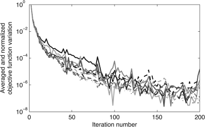
The convergence criterion is plotted versus the iteration number for several values of λ in Fig. 1. Notice that the convergence rate is similar for several values of λ. In practice, a threshold of 10−3 is used to define convergence.
Figure 1.
Plot of the convergence criterion value, the variation averaged every two iterations, with respect to the iteration number. Each line corresponds to a different value of the data consistency parameter λ in the range [103,108].
Each algorithm was applied to the PICCS objective function for 16 different values of λ on a logarithmic scale from approximately 3 × 10³–4 × 10¹⁰. The prior image parameter α was set to 0.5. The rRMSE was measured for all the reconstructions once convergence had been reached. The means and standard deviations of the rRMSE for each algorithm are given in Table TABLE I.. One notices that the reconstruction accuracy is very similar for all algorithms studied. Furthermore, only small fluctuations in accuracy are observed, as the standard deviation is relatively constant. One must note that a portion of the rRMSE is due to the noise present in the fully-sampled FBP reconstructions used as a reference. A portion is also caused by mismatches in spatial resolution at edges. This explains the relatively high values measured for all the algorithms.
Table 1.
Algorithms performance comparison.
| Algorithm | Mean rRMSE at convergence | Mean number of CG iterations before convergence | Mean number line search iterations |
|---|---|---|---|
| SD–BT | 10.9 ± 0.5% | 68 ± 22 | 22 ± 3 |
| CG–FR–BT | 10.1 ±0.8% | 27 ± 4 | 12.5 ± 0.9 |
| CG–PR–BT | 10.6 ± 0.7% | 31 ± 15 | 16 ± 9 |
| SD–NR | 11.2 ±0.5% | 47 ± 16 | 0 ± 0 |
| CG–FR–NR | 10.0 ± 0.9% | 15 ± 2 | 0.01 ± 0.02 |
| CG–PR–NR | 10.2 ± 0.7% | 15 ± 1 | 0.01 ± 0.01 |
The convergence speed is where the algorithms show substantial differences. The comparison is drawn from the number of iterations necessary to reach convergence (Table TABLE I.). The steepest descent (SD) methods show the slowest convergence with a number of iterations two to three times greater than for CG algorithms. Fletcher-Reeves and Polak-Ribiere formulas perform equally well in terms of convergence speed.
The advantage of the NR line search over the backtracking (BT) line search is threefold. First, it cuts the number of CG iterations needed for convergence by half. Second, it converges more predictably, which is shown by the lower standard deviation in the mean number of iterations. These advantages are due to the nature of the BT line search, in that it systematically overshoots the position of the objective function minimum while, the NR line search attempts to estimate the position of the minimum and generates a greater diminution in the objective function at most iterations. Third, it is shown in (Table TABLE I.) that the NR line search requires line searching in less than 1% of the CG iterations performed. The BT line search generally requires several iterations before it discovers a step size that generates a sufficient reduction in the objective function. While this is due in part by the choice of a large initial step size guess for the BT algorithm, we still conclude that the NR line search—with its near zero number of line searches—is superior.
Based on these findings, CG–FR–NR is determined to be superior and is used for the rest of the studies. The Fletcher-Reeves formula is chosen over the Polak-Ribiere formula because of its lower memory requirements.
Performance dependence of parameters in the PICCS objective function
Numerical datasets
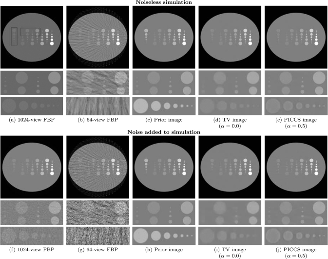
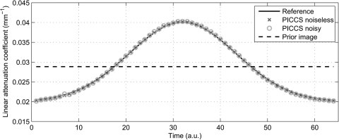
The simulated projection datasets were reconstructed using PICCS for a range of α and λ parameters. Some sample images are presented in Fig. 2 for both the noiseless and noisy datasets. The prior image was produced by averaging over images reconstructed using FBP from the 64 view angle datasets of all 64 time frames. An interleaved sampling pattern was used among all 64 time frames. Thus, the averaging procedure mitigated the undersampling artifacts present in each individual time frame. In contrast, the reference images were reconstructed using FBP from the 1024 view angle datasets at each time frame. Notice the difference in contrast of the dynamic structure regions between the reference and prior images. The contrast from particular time frames was accurately reconstructed in TV minimization and PICCS reconstructions. The average attenuation coefficients within the largest dynamic object were measured for all time frames reconstructed using PICCS and are plotted in Fig. 3. Notice that the PICCS images show a slight amount of edge enhancement around the dynamic structures. This inaccuracy is quantified by an increase in the rRMSE in the corresponding ROI as α increases.
Figure 2.
Reconstructions of the numerical phantom using FBP, TV minimization, and PICCS for two values of the prior image parameter α. The prior image used for the PICCS reconstructions is shown. Notice that at α = 0.0, the image lacks fine details. At α = 0.5, the image accurately shows small scale details at all contrasts levels. The display range is set to [0.00, 0.04] mm−1.
Figure 3.
Plot of the contrast enhancement of the dynamic numerical phantom at various time frames.
An important point to notice about the TV minimization images (α = 0) shown in Fig. 2 is the loss of small scale, low-contrast details in the static region of the phantom. This region was reconstructed sharply in the PICCS reconstructions at α = 0.5. This results was expected since that region of the image was accurately reconstructed in the prior image. To quantify this behavior, the rRMSE was measured in an ROI which included only these static structures [Fig. 4a]. This analysis was done for the noiseless dataset to remove the effect of noise. The error is reduced as α increased. However, the error measured in an ROI around the dynamic structures increases with α. Therefore, there exists a trade-off between the accuracy of static and dynamic structures.
Figure 4.
Plots of quantitative metrics with respect to variations in the prior image parameter α for the noiseless numerical phantom at 64 projection view angles. (a) shows the rRMSE measures within two ROIs each containing either static or dynamic structures [see Figs. 2a]. (b) shows spatial resolution measurements of the smallest static structure for various contrast levels. (c) shows spatial resolution measurement for the lowest contrast static objects for several sizes. Note that the pixel size is (1 mm)2.
Furthermore, the spatial resolution of the image was shown to depend on the object size and contrast. Figures 4b, 4c show the pseudo PSF width as a function of α for static objects of different sizes and contrast levels. Small and low-contrast objects are preferably blurred by TV minimization. These results clearly demonstrate that the point spread function of images reconstructed using TV minimization or PICCS is not shift-invariant. When α was increased above 0.5, the spatial resolution of small low-contrast objects was restored; that is, the pseudo PSF width dropped below the pixel size, (1 mm)2. For α = 0.5 and above, the spatial resolution is below the pixel size (1 mm)2 for all values of A studied. As λ is decreased, the noise level converges to that of the prior image 1.5 × 10⁻⁴ mm−1.
The dataset with noise added was also analyzed with respect to spatial resolution. TV minimization images with noise showed deformed low-contrast structures due to patchy artifacts. The same contrast and size dependence of the resolution was observed in that case. Figure 5 demonstrates the tradeoff between noise and spatial resolution for low, medium, and high contrast objects. Notice the characteristic L-shape of these curves. For large values of λ, the noise level varies without loss of spatial resolution. However, at low values of λ and α, the pseudo PSF width increases without an improvement in noise level. This figure demonstrates that PICCS with properly selected parameters offers a reduction in noise with respect to the FBP reconstructed reference image without a loss in spatial resolution around low-contrast static objects.
Figure 5.
Plot of the noise standard deviation as a function of the pseudo PSF width for the numerical phantom with noise added. Each point of a given curve corresponds to a different value of λ ∈ {0.46,0.90, 2.2, 5.4,13, 32}, is shown for all values of α. The pseudo PSF in (a) is for a low-contrast object while that in (b) is for a medium contrast object and (c) is for a high contrast object. Note that the prior image has a noise standard deviation of 1.5 × 10⁻⁴ mm−1 and a pseudo PSF width of 0.1 mm which is negligible compared with the pixel size of 1 mm. Similarly, the potential blur of the PICCS reconstructed images is also negligible at the optimal value of α = 0.5.
In vivo dataset
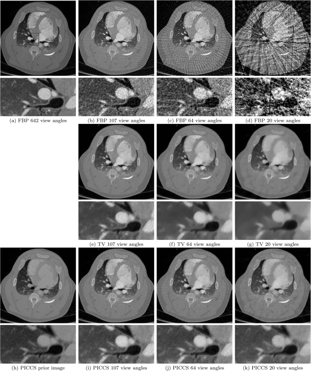
Reconstructions were performed for a range of α from 0 to 1 by 0.1 increments at various values of λ using the in vivo dataset. Reconstructions at several sampling levels are shown on Fig. 6. Notice that image quality depends on the sampling level. At 107 view angles, the TV minimization image showed high accuracy but a slightly patchy texture. As the sampling level is further reduced to 64 and 20 view angles, the spatial resolution is degraded in the lung region and the texture becomes overly smooth. For PICCS images, the texture of the lung region remains qualitatively similar to that of FBP images. There is a minimal loss of spatial resolution obeserved in the 20-view angle PICCS reconstruction in the ventricular and pulmonary regions. However, this loss is minor in comparison to that suffered by TV minimization images.
Figure 6.
Reconstructions of the invivo study using FBP, TV minimization, and PICCS. At all sampling rates shown here, FBP images show undersampling artifacts in the form of streaks. For TV minimization (α = 0.0), the image lacks fine details and has an overly smooth texture for sampling rates below 100 view angles. Using PICCS (α = 0.5), images accurately show small scale details with minimal loss at all sampling levels. The display range is set to [−1000,1000] HU.
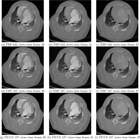
To qualitatively evaluate the temporal resolution, reconstructions at three different time frames for the 64 view angle dataset using optimal parameters are presented in Fig. 7. Notice the change in the contrast of the cardiac chambers as the concentration of iodinated agent varies.
Figure 7.
Reconstructions for various time frames following contrast injection. The complete dataset had 66 time frames. The display range is set to [−1000,1000] HU. The PICCS images were produced from datasets with 107 view angles, while those used for the FBP images had either 642 or 107 view angles.
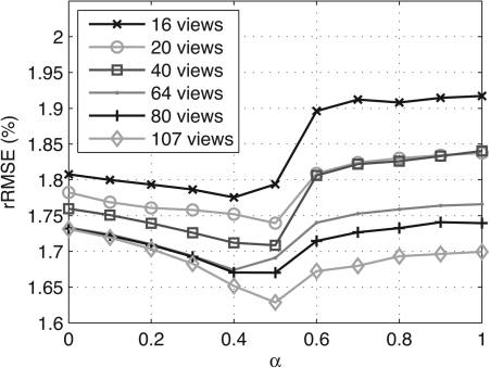
In order to evaluate the accuracy of the reconstruction, the rRMSE was measured for all images within an ROI that included soft tissue only, thus excluding the lungs and bones. These regions are excluded since sharp interfaces are present that could generate artificially high rRMSEs due to mismatches in spatial resolutions between the reconstructions and the reference image. The rRMSE is plotted with respect to the α parameter for various levels of view angle sampling (Fig. 8). For each curve, the data consistency parameter λ that offered the minimal rRMSE was used. A striking feature of these curves is the presence of an optimal value of the prior image parameter. Indeed, the rRMSE is lowest for values of α between 0.4 and 0.5. This behavior is well correlated by the qualitative appearance of the reconstructions. At low α, the reconstructions are overly smooth, which causes a loss in fine, low-contrast structures. At large α, the algorithm applies an excessive weight on the prior image conformity, and thus, it retains some of the prior image features. At the optimal α, details are accurately reconstructed and the prior image is minimally visible.
Figure 8.
Plots of the relative root mean square error with respect to the prior image parameter α. Each curve corresponds to a different level of sampling. Note that the prior image used in all cases had a rRMSE of 2.31%.
As the number of projection view angles is reduced the rRMSE increases since PICCS looses some of its ability to correct for inconsistencies between the prior image and the projection data. However, at all sampling levels, a PICCS reconstruction yields an accuracy superior to that of TV minimization. These results are consistent with the rRMSE measurements obtained for the noiseless simulated dataset [Fig. 4a]. For the in vivo dataset, the ROI contained both static and dynamic structures. The rRMSE thus combined the behavior of both curves from Fig. 4a.
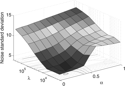
The level of noise present in the images also depends on the prior image parameter α. At low α, the noise is mitigated by the total variation term of the PICCS objective function, while at larger values, it has a level similar to the one found in the prior image (Fig. 9).
Figure 9.
Surface plot of the noise standard deviation in HU as a function of the prior image parameter α and the data consistency parameter λ. The noise standard deviation in the prior image is 9.35 HU. This figure was generated using data measured from the reconstructions of the 107-view angle dataset. Similar results can be obtained for other sampling factors.
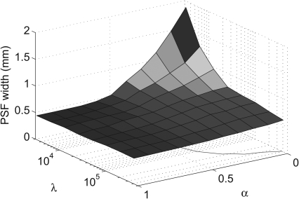
As previously observed, lower noise comes at a price. Low-contrast details are often lost. This behavior is quantified by the pseudo PSF width (Fig. 10), which was measured at 18% contrast interfaces. At moderate to high values of α, the spatial resolution is preserved. However, when α is low, the total variation term of the objective function dominates, and the width of the pseudo PSF increases. This means that low-contrast spatial resolution is being degraded.
Figure 10.
Surface plot of the pseudo point spread function (PSF) width as a function of the prior image parameter α and the data consistency parameter λ. The width of the pseudo PSF in the prior image is 0.45 mm. Note that this plot is rotated by 180° with respect to (Fig. 9) to allow better visualization. This figure was generated using data measured from the reconstructions of the 107-view angle dataset. Similar results can be obtained for other sampling factors.
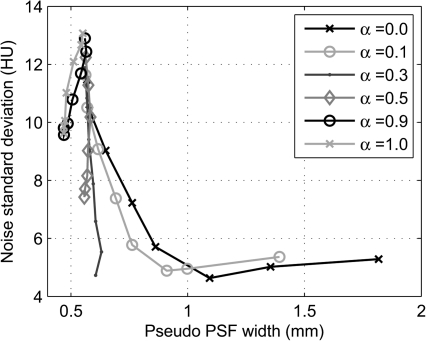
There exists a trade-off between the loss of spatial resolution and the noise level. This is illustrated in Fig. 11. Each curve corresponds to a different value of α, while the points on a given curve correspond to different values of λ. One important observation to be made from the figure is that for large enough values of α, the pseudo PSF width is relatively constant for all values of λ.
Figure 11.
Plot of the noise standard deviation as a function of the pseudo PSF width. The pseudo PSF measurements were performed at a low-contrast edge in soft tissue. This figure was generated using data measured from the reconstructions of the 107-view angle dataset. In the prior image, the pseudo PSF width is 0.45 mm and the noise standard deviation is 9.35 HU. Similar results can be obtained for other sampling factors.
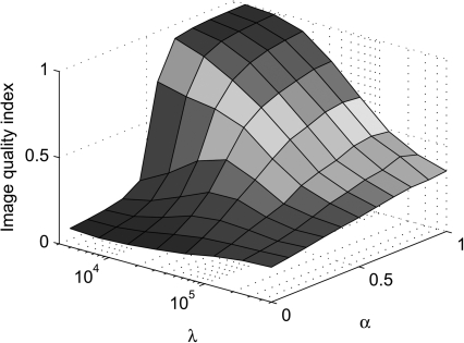
The texture of the images also varies considerably for different values of α. At the low end, images show a step-like appearance and often show patchy artifacts. As α is increased, the texture of PICCS-reconstructed images becomes more similar to that of FBP-reconstructed images. This is quantified by the QI shown on Fig. 12. At α ≥ 0.5, the QI was close to 1, which signifies a level of high texture conformity with the reference image. It is also interesting to note that as λ is increased, the noise texture of the images resembles more and more the texture of FBP images. The QI is sensitive to the noise level. At high λ, the noise increases beyond the level of the reference image, which causes a decrease in QI.
Figure 12.
Surface plot of the universal image quality index as a function of the prior image parameter α and the data consistency parameter λ.
The appearance of in vivo images also varies with respect to the value of the data consistency parameter λ. For low values of λ, the difference between various α levels, in terms of noise, and spatial resolution is maximized. These differences reduce gradually as λ increases. It is reasonable to attribute this behavior to the fact that at large values of λ the algorithm converges approximately to the solution of the least squares problem
| (23) |
In this regime, variations in the PICCS objective function fpiccs(x) have little impact on the reconstructions. The data consistency parameter λ should be kept at a lower level in order to retain the advantages of PICCS with respect to noise suppression and under-sampling artifacts mitigation. However, in that regime, less weight is given to the consistency of the image with the projection dataset.
In summary, it was also shown in this section that a value of α near 0.5 is an optimal choice with respect to reconstruction accuracy, the trade-off between noise level and low-contrast spatial resolution, as well as image texture.
CONCLUSIONS AND DISCUSSION
Various classical unconstrained optimization algorithms were implemented to minimize the PICCS objective function. When applied to a porcine CT dataset acquired in vivo, it was shown that the nonlinear conjugate gradient algorithm with a fast Newton-Raphson line search displayed the fastest convergence speed with proper accuracy. Using this algorithm, the parameters of the unconstrained PICCS objective function were studied. For both numerical and in vivo datasets, it was shown that a value of α around 0.5 is an optimal choice with respect to both the reconstruction accuracy and the trade-off between noise level and low-contrast spatial resolution. This value of α also results in sharp low-contrast details. Using the in vivo dataset, it was also shown that this choice of α results in a noise texture similar to that of FBP images. Finally, it was demonstrated that the data consistency parameter λ should be kept at a lower level in order to retain the advantages of the PICCS framework with respect to noise suppression and under-sampling artifacts mitigation.
One limitation of the present study is that an explicit noise model is not included in the PICCS objective function [Eq. 6]. As mentioned in Sec. 1, the introduction of a noise model can become important in ultralow-dose CT. The performance of PICCS is not expected to change, with the exception of better noise performance. However, it would be interesting for future investigations to see how much advantage can be gained by the incorporation of a detailed noise model in PICCS framework.
Another limitation of the present study is that the topic of how “good” the prior image should be in order for PICCS to yield high performance. This aspect was not discussed here. In published results so far, PICCS is well suited for applications where a prior image with compromised temporal resolution, spectral resolution, and/or spatial resolution, but also a high SNR can be generated from the acquired projection data. The generalization to a more general prior image remains an interesting research topic for future investigations.
ACKNOWLEDGMENTS
The work is partially supported by the National Institutes of Health through R01EB009699, Varian Medical Systems, and a doctoral scholarship from NSERC-CRSNG (P.T.L.). The authors wish to thank Nicholas Bevins for his editorial input. The authors also wish to express their gratitude to anonymous reviewers for their thoughtful comments and suggestions.
References
- Gordon R., Bender R., and Herman G., “Algebraic reconstruction techniques (ART) for three-dimensional electron microscopy and x-ray photography,” J. Theor. Biol. 29, 471–481 (1970). 10.1016/0022-5193(70)90109-8 [DOI] [PubMed] [Google Scholar]
- Herman G., Image Reconstruction From Projections, 2nd ed. (Springer, New York, 2009). [Google Scholar]
- Andersen A. and Kak A., “Simultaneous algebraic reconstruction technique (SART): A superior implementation of the ART algorithm,” Ultrason. Imaging 6, 81–94 (1984). 10.1016/0161-7346(84)90008-7 [DOI] [PubMed] [Google Scholar]
- Gabor T. C. et al. , “On some optimization techniques in image reconstruction from projections,” Appl. Numer. Math. 3, 365–391 (1987). 10.1016/0168-9274(87)90028-6 [DOI] [Google Scholar]
- Jiang M. and Wang G., “Convergence of the simultaneous algebraic reconstruction technique (SART),” IEEE Trans. Image Process. 12, 957–961 (2003). 10.1109/TIP.2003.815295 [DOI] [PubMed] [Google Scholar]
- Jiang M. and Wang G., “Convergence studies on iterative algorithms for image reconstruction,” IEEE Trans. Med. Imaging 22, 569–579 (2003). 10.1109/TMI.2003.812253 [DOI] [PubMed] [Google Scholar]
- Wang G. and Jiang M., “Ordered-subset simultaneous algebraic reconstruction techniques (OS-SART),” J. X-Ray Sci. Technol. 12 (3), 169–177 (2004). [Google Scholar]
- E. Candés, Romberg J., and Tao T., “Robust uncertainty principles: Exact signal reconstruction from highly incomplete frequency information,” IEEE Trans. Inf. Theory 52, 489 (2006). 10.1109/TIT.2005.862083 [DOI] [Google Scholar]
- Candes E., Romberg J., and Tao T., “Stable signal recovery from incomplete and inaccurate measurements,” Commun. Pure Appl. Math. 59, 1207–1223 (2006). 10.1002/cpa.v59:8 [DOI] [Google Scholar]
- Donoho D., “Compressed sensing,” IEEE Trans. Inf. Theory 52, 1289–1306 (2006). 10.1109/TIT.2006.871582 [DOI] [Google Scholar]
- Chen G., Tang J., and Leng S., “Prior image constrained compressed sensing (PICCS): A method to accurately reconstruct dynamic CT images from highly undersampled projection data sets,” Med. Phys. 35, 660 (2008). 10.1118/1.2836423 [DOI] [PMC free article] [PubMed] [Google Scholar]
- Leng S., Tang J., Zambelli J., Nett B., Tolakanahalli R., and Chen G., “High temporal resolution and streak-free four-dimensional cone-beam computed tomography,” Phys. Med. Biol. 53, 5653 (2008). 10.1088/0031-9155/53/20/006 [DOI] [PMC free article] [PubMed] [Google Scholar]
- Qi Z. and Chen G.-H., “Extraction of tumor motion trajectories using prior image constrained compressed sensing based four-dimensional cone beam CT (PICCS-4DCBCT): A validation study,” Med. Phys. 38, 5530 (2011). 10.1118/1.3637501 [DOI] [PMC free article] [PubMed] [Google Scholar]
- Qi Z. and Chen G.-H., “Performance studies of PICCS based four dimensional cone beam computed tomography (PICCS-4DCBCT),” Phys. Med. Biol. 56, 6709 (2011). 10.1088/0031-9155/56/20/013 [DOI] [PMC free article] [PubMed] [Google Scholar]
- Chen G., Tang J., and Hsieh J., “Temporal resolution improvement using PICCS in MDCT cardiac imaging,” Med. Phys. 36, 2130 (2009). 10.1118/1.3130018 [DOI] [PMC free article] [PubMed] [Google Scholar]
- Tang J., Hsieh J., and Chen G., “Temporal resolution improvement in cardiac CT using PICCS (TRI-PICCS): Performance studies,” Med. Phys. 37, 4377 (2010). 10.1118/1.3460318 [DOI] [PubMed] [Google Scholar]
- Szczykutowicz T. and Chen G., “Dual energy CT using slow kVp switching acquisition and prior image constrained compressed sensing,” Phys. Med. Biol. 55, 6411 (2010). 10.1088/0031-9155/55/21/005 [DOI] [PubMed] [Google Scholar]
- Nett B., Brauweiler R., Kalender W., Rowley H., and Chen G., “Perfusion measurements by micro-CT using prior image constrained compressed sensing (PICCS): Initial phantom results,” Phys. Med. Biol. 55, 2333 (2010). 10.1088/0031-9155/55/8/014 [DOI] [PMC free article] [PubMed] [Google Scholar]
- Tang J., Lauzier P. T., and Chen G., “Dose reduction using prior image constrained compressed sensing (DR-PICCS),” Proc. SPIE 7961, 79612K (2011). 10.1117/12.878200 [DOI] [Google Scholar]
- Lubner M., Pickhardt P., Tang J., and Chen G., “Reduced image noise at low-dose multi-detector ct of the abdomen with prior image constrained compressed sensing algorithm,” Radiology 260, 248 (2011). 10.1148/radiol.11101380 [DOI] [PubMed] [Google Scholar]
- Ramirez-Giraldo J., Trzasko J., Leng S., McCollough C., and Manduca A., “Non-convex prior image constrained compressed sensing (NC-PICCS),” Proc. SPIE, 7622, 76222C (2010). 10.1117/12.837239 [DOI] [Google Scholar]
- Ramirez-Giraldo J., Trzasko J., Leng S., Yu L., Manduca A., and McCollough C., “Non-convex prior image constrained compressed sensing (NCPICCS): Theory and simulations on perfusion CT,” Med. Phys. 38, 2157 (2011). 10.1118/1.3560878 [DOI] [PMC free article] [PubMed] [Google Scholar]
- Sidky E. and Pan X., “Image reconstruction in circular cone-beam computed tomography by constrained, total-variation minimization,” Phys. Med. Biol. 53, 4777 (2008). 10.1088/0031-9155/53/17/021 [DOI] [PMC free article] [PubMed] [Google Scholar]
- Sidky E., Pan X., Reiser I., Nishikawa R., Moore R., and Kopans D., “Enhanced imaging of microcalcifications in digital breast tomosynthesis through improved image-reconstruction algorithms,” Med. Phys. 36, 4920 (2009). 10.1118/1.3232211 [DOI] [PMC free article] [PubMed] [Google Scholar]
- Ritschl L., Bergner F., Fleischmann C., and Kachelrieß M., “Improved total variation-based ct image reconstruction applied to clinical data,” Phys. Med. Biol. 56, 1545 (2011). 10.1088/0031-9155/56/6/003 [DOI] [PubMed] [Google Scholar]
- Song J., Liu Q., Johnson G., and Badea C., “Sparseness prior based iterative image reconstruction for retrospectively gated cardiac micro-CT,” Med. Phys. 34, 4476 (2007). 10.1118/1.2795830 [DOI] [PMC free article] [PubMed] [Google Scholar]
- Choi K., Wang J., Zhu L., Suh T., Boyd S., and Xing L., “Compressed sensing based cone-beam computed tomography reconstruction with a first-order method,” Med. Phys. 37, 5113 (2010). 10.1118/1.3481510 [DOI] [PMC free article] [PubMed] [Google Scholar]
- Nesterov Y., “Gradient methods for minimizing composite objective function,” Technical Report (Center for Operations Research and Econometrics (CORE), Universite Catholique de Louvain, 2007).
- Bian J., Siewerdsen J., Han X., Sidky E., Prince J., Pelizzari C., and Pan X., “Evaluation of sparse-view reconstruction from flat-panel-detector cone-beam CT,” Phys. Med. Biol. 55, 6575 (2010). 10.1088/0031-9155/55/22/001 [DOI] [PMC free article] [PubMed] [Google Scholar]
- Thibault J., Sauer K., Bouman C., and Hsieh J., “A three-dimensional statistical approach to improved image quality for multislice helical CT,” Med. Phys. 34, 4526 (2007). 10.1118/1.2789499 [DOI] [PubMed] [Google Scholar]
- Tang J., Nett B., and Chen G., “Performance comparison between total variation (TV)-based compressed sensing and statistical iterative reconstruction algorithms,” Phys. Med. Biol. 54, 5781 (2009). 10.1088/0031-9155/54/19/008 [DOI] [PMC free article] [PubMed] [Google Scholar]
- Rudin L., Osher S., and Fatemi E., “Nonlinear total variation based noise removal algorithms,” Physica D: Nonlinear Phenom. 60, 259–268 (1992). 10.1016/0167-2789(92)90242-F [DOI] [Google Scholar]
- Ascher U., Haber E., and Huang H., “On effective methods for implicit piecewise smooth surface recovery,” SIAM J. Sci. Comput. 28, 339 (2006). 10.1137/040617261 [DOI] [Google Scholar]
- Nocedal J. and Wright S., Numerical Optimization (Springer, New York, 1999). [Google Scholar]
- Shewchuk J., “An introduction to the conjugate gradient method without the agonizing pain,” (1994), http://www.cs.cmu.edu/~quake-papers/painless-conjugate-gradient.pdf by the School of Computer Science at Carnegie Mellon University.
- Hestenes M. and Stiefel E., “Methods of Conjugate Gradients for Solving Linear Systems,” J. Res. Natl. Bur. Stand. 49 409–436 (1952). [Google Scholar]
- Fletcher R. and Reeves C., “Function minimization by conjugate gradients,” Comput. J. 7, 149–154 (1964). 10.1093/comjnl/7.2.149 [DOI] [Google Scholar]
- Polak A. and Ribiére , “Note sur la convergence de méthodes de directions conjuguées,” Revue frangçaise d’informatique et de recherche opérationnelle 3, 35–43 (1969). [Google Scholar]
- Powell M., “Restart procedures for the conjugate gradient method,” Math. Program. 12, 241–254 (1977). 10.1007/BF01593790 [DOI] [Google Scholar]
- Vogel C. and Oman M., “Iterative methods for total variation denoising,” SIAM J. Sci. Comput. 17, 227–238 (1996). 10.1137/0917016 [DOI] [Google Scholar]
- Vogel C. and Oman M., “Fast, robust total variation-based reconstruction of noisy, blurred images,” IEEE Trans. Image Process. 7, 813–824 (2002). 10.1109/83.679423 [DOI] [PubMed] [Google Scholar]
- Wang Z. and Bovik A., “A universal image quality index,” IEEE Signal Process. Lett. 9, 81–84 (2002). 10.1109/97.995823 [DOI] [Google Scholar]


