

Abstract
Eukaryotic genome is organized in a set of chromosomes each of which consists of a chain of DNA and associated proteins. Processes involving DNA such as transcription, duplication, and repair, therefore, should be intrinsically related to the three-dimensional organization of the genome. In this article, we develop a computational model of the three-dimensional organization of the haploid genome of interphase budding yeast by regarding chromosomes as chains moving under the constraints of nuclear structure and chromatin-chromatin interactions. The simulated genome structure largely fluctuates with the diffusive movement of chromosomes. This fluctuation, however, is not completely random, as parts of chromosomes distribute in characteristic ways to form “territories” in the nucleus. By suitably taking account of constraints arising from the data of the chromosome-conformation-capture measurement, the model explains the observed fluorescence data of chromosome distributions and motions.
Introduction
Genome is not an abstract linear sequence but has a physical structure organized in the three-dimensional space. In eukaryotic cells, DNA folds hierarchically into several layers from chromatin to chromosome and to the whole genome, so that the DNA-related processes such as transcription, duplication, and repair should be affected or regulated by the three-dimensional organization of the genome (1, 2, 3, 4): It has been observed, for instance, that the disparate DNA elements colocalize in interphase nuclei to form “transcription factories” (5). Such structure of interphase chromosomes, however, is not a frozen static configuration but is subject to the intense dynamical fluctuation.
In one view, this dynamical motion has been ascribed to the random movement of chromosome chains. In the human genome, for example, the observation based on the chromosome conformation capture (3C) method (6) has shown that the genome is organized as a fractal globule (7) whose features are well reproduced by the Monte Carlo simulation of the randomly moving nonspecific polymer chains (6, 8). Rosa and Everaers (9) and Rosa et al. (10) have extended the wormlike chain model of semiflexible polymers to describe chromosomes and shown that a nonspecific kinetic effect of the Brownian motion of chromosome chains can separate different parts of the genome into “territories”. Also in the genome of budding yeast, observation of the GFP-tagged loci has shown that each chromosome moves ∼0.5 μm during 10 s—almost half of the radial length of the nucleus (11, 12, 13). The recent fluorescence measurement has shown that the positional distribution of telomeres widely spreads in the interphase yeast nucleus but is largely determined by the arm-length of each chromosome (14, 15). These results suggest that the important features of interphase nuclei can be captured by regarding nuclei as solutions of nonspecific polymers (9, 16).
In the other view, the genome structure has been regarded as an ensemble of configurations that are constrained by specific interactions between chromosomes and the nuclear structure (3, 17, 18) and also by specific interactions among chromosomes (1). In yeast, for example, centromeres are anchored to the spindle pole body (SPB), a protein structure embedded in the nuclear envelope (17, 19, 20). The repetitive elements of ribosomal DNA (rDNA) are confined in the nucleolus that is positioned at the opposite side of the nucleus from SPB (17, 20, 21). These constraints should break symmetry of the chromosome distribution to give rise to the “Rabl-like” structure, which has been recently confirmed by the 3C-based measurement (22). By using the 3C-based methods, the frequency that two positions of chromosomes approach in proximity has been measured with the kilobase pair (kbp) resolutions, from which three-dimensional models of genome structure have been constructed for budding yeast (22) and fission yeast (23). It has been reported that for fission yeast thus observed, proximity and the expression pattern of genes are correlated to each other, and those significantly associating genes frequently contain the same DNA motifs at their promoter regions (23). Tanizawa et al. (23) have suggested that putative specific factors binding to these motifs are involved in defining the associations among genes. Upon induction of double-strand break (DSB), it has been observed that two loci colocalize to form a focus with proteins of the repair machinery (24). These examples have shown the importance of specific interactions between loci and between locus and a nuclear landmark (4).
By unifying these two views, the view based on the polymer dynamics and the view based on the specific interactions, it should become possible to examine intriguing and important questions on how the Rabl-like global structure is maintained or changed and how the specific local structures are formed or dissolved under the intense dynamical fluctuation. Computer modeling should be an efficient approach to explore this problem, and in this article, we introduce a computational model of the three-dimensional genome organization in the interphase nucleus of haploid budding yeast. As has been pointed out by Grosberg et al. (7) and Marti-Renom and Mirny (25), this problem resembles, in a sense, the problem of protein folding: In these problems, both the polymer dynamics and the specific interactions are important, and hence we here borrow the idea of structural modeling from protein folding study (26).
The 3C-based methods have provided information of the frequency that two sites in the genome come close to each other. From such frequencies, Duan et al. (22) estimated mean distances between sites in the interphase haploid budding yeast. We use these distances to define the Gō-like potential for genome. In the problem of protein folding, a simulated protein folds into the unique structure that minimizes the Gō-like potential when the balance between temperature and the interaction energy in the model is favorable for folding (27, 28). In the condition that favors the more loosened structure, i.e., in high temperature or with the small interaction parameters, the protein chain does not settle in a folded structure, but in this case the Gō-like potential suitably describes the statistical tendency of large conformational fluctuations around the mean structure (26, 28). In the similar way, for the genome problem, we expect that the large fluctuation of chromosomes around their mean structures can be suitably described with the Gō-like potential although chromosomes do not fold into unique structures in the nucleus.
With this method we investigate the chain dynamics of chromosomes when specific interactions work in the nucleus. This method should provide a platform to examine which interactions are necessary to explain the observed structural data and which features of the genome structure are the consequences of the random Brownian motions of chromosome chains. We find necessary conditions that the model has to meet to explain the observed fluorescently visualized data of the genome structure and dynamics in a consistent way; especially the distribution of the distance between telomeres and the dynamical feature of moving telomeres are compared with the experimental data. The results presented here show that the dynamical structural modeling is a step forward to construct a unified view of the genome organization.
Methods
The bead-spring polymer model
In our model, 16 chromosomes in the interphase haploid budding yeast are represented by 16 chains of beads and springs. Because the observed data of pairwise mean distances have resolution of a few kbp (22), we assume that each bead in the model corresponds to a 3-kbp DNA segment. Each chromosome consists of 78 (Chromosome 1, or Chr1) to 806 (Chr12) beads and the total 4460 beads are considered for 16 chains.
Movement of each chromosome chain is simulated by the Langevin dynamics that is obtained by numerically solving the equation of motion,
| (1) |
where riμ is the position of the ith bead of the μth chain with μ = 1–16, m is the mass of a bead, and ζ is the friction coefficient. The vector wiμ is the Gaussian white noise with the dispersion
where α and β represent the x, y, or z component of the vector. Movement of chromosomes in the interphase yeast nucleus is the nonequilibrium process whose rate depends on the ATP concentration (11, 12). This energy-dependent motion, however, is random and is brought about without any detectable large motor system that may generate the coherent biased motion (12). We therefore conveniently simulate this random motion by using the effective temperature T (with the unit of kB = 1) though the explicit consideration of the nonequilibrium effects should be important in the future research. Hereafter, T is used as a unit to define interaction parameters in U.
The potential U consists of several terms,
| (2) |
where the first three terms represent the extended version of the wormlike chain model that includes a kinkable potential as explained later in this subsection.
The term ULJ consists of purely repulsive Lennard-Jones (LJ) type potentials representing the exclusive forces between chromatins,
| (3) |
where ULJ(μ,i;ν,j) has the same functional form as used by Rosa et al. (10):
| (4) |
Here, , and a is the thickness of the chromatin fiber, where a = 30 nm, with the exception explained later in Simulation. When the ordered chromatin structure is modified through fluctuation, two chromatin fibers may come closer than a (16). We adopt a mild value of ϵ/T = 1 to allow two chromatin chains to approach each other.
Uspring is the potential to describe the spring between neighboring beads along the chain,
| (5) |
where , and when and when . Here, UFENE is the finitely extensible nonlinear elastic (FENE) potential (9, 10, 29):
| (6) |
Following Rosa et al. (10), we chose R0 to be R0 = 1.5σ0 with σ0 being the typical length of the spring. By assuming the packing density of chromatin as 130 bp/nm (19), σ0 ≈ 3000/130 = 23 nm, so that R0 = 34.5 nm. The value k was calibrated to be k/T = 3.5/σ02 so as to make the simulated mean distance between neighboring beads to be σ0. The FENE potential of Eq. 6 diverges at ∼R0. To avoid the numerical instability due to this divergence, the potential is switched in Eq. 5 to the milder one as Ul = (bk/σ02) (riμ)5 for riμ ≥ R0′ = 30 nm. For the smooth connection in this switching, we use b = 0.42. To keep the numerical stability, we also introduce a mild repulsive potential Ur in Eq. 5 as
| (7) |
The potential represents the stiffness of chromatin fibers, where ϕiμ is the angle between vectors and . Because the local cooperative rearrangement of nucleosomes should bring about the sharp bending, or the kink of the chromosome (30, 31), we use a kinkable bending potential that saturates for ϕ > π/2 (10, 32) as
| (8) |
where the boundary value of 0.1 was chosen to fit Ub to the potential proposed in Rosa et al. (10), but its precise value does not affect the results. The dispersion of angles should be related to the persistent length lp and σ0 as 〈ϕ2〉 ≥ 2σ0/lp (33). Using the estimation of lp ≈ 170–220 nm for chromatins (19) and σ0 ≈ 23 nm, we have . The value kϕ was calibrated to be kϕ/T = 2.0 to make the simulated results of fall in this range.
The Gō-like potential
UGō in Eq. 2 is the potential representing the tendency that distances between sites of chromosomes fluctuate around the mean distances estimated from the 3C-based method (22). We derive σijμν, the mean distance between the ith site of the μth chromosome and the jth site of the νth chromosome, by using the curve of Supplementary Fig. 17 of Duan et al. (22) to transform the measured frequency of proximate contact into the mean distance. Using thus derived σijμν, we have
| (9) |
with
| (10) |
Here, to simulate the large fluctuation in rijμν, a shallow Gaussian function with c = 0.1 is used instead of the short-ranged Lennard-Jones type potential that is more popular in Gō-like models (28). The similar Gaussian potentials for pairwise distances have been used in the structural modeling of proteins (34, 35, 36).
Because σijμν is determined by the combined effects of the specific chromatin-chromatin interactions, the specific chromatin-nucleus interactions, and the random movement of chromosome chains, the lower value of UGō indicates that the consistency among those effects is better fulfilled in the model. As compared with the effects of the chromatin-nucleus interactions and the kinetic effects represented by Unucleus and ULJ + Uspring + Ubend, respectively, UGō highlights the effects of specific chromatin-chromatin interactions that may arise, for example, from the transient formation of protein complexes that bind multiple chromosomes together. In this article we compare the results by varying ξ in Eq. 10 to see the roles of the chromatin-chromatin interactions in organization of the genome.
Constraint of nuclear structure
The nuclear structure considered in the model is illustrated in Fig. 1. We use the coordinate shown in Fig. 1 to explain the structure. The nucleus of interphase budding yeast is approximated by a sphere of 1 μm (11, 17), so that the center of nucleus is placed on rcenter = (1000,1000,1000) in units of nanometers. The observed position of SPB is ∼13 nm away from the nuclear envelope (17), so that we approximate the position of SPB as (1000,1000,10).
Figure 1.
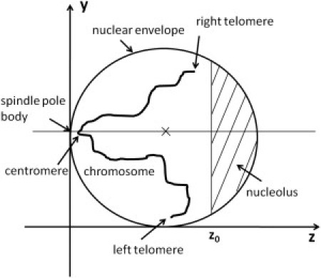
Yeast nucleus is approximated by a sphere of radius 1 μm. Center of the sphere (marked by a cross) is at (1000,1000,1000) in units of nanometers in the model coordinate. Nucleolus is represented by the region of z > z0. One of 16 chromosomes (Chr10) is schematically drawn in the figure. Centromere of each chromosome is linked to spindle pole body (SPB), which is a protein complex embedded in the nuclear envelope, and termini of each chromosome are left and right telomeres.
Centromeres of chromosomes are linked to SPB with microtubules. This linkage is represented by the potential for spring as
| (11) |
where lμ is the length between SPB and the centromere of the μth chromosome and l0μ is the corresponding length defined in the model structure of Duan et al. (22). The spring constant h is chosen to allow the length variation of linker microtubules as h/T = 0.3 with s = 100 nm. This small stiffness should make positions of centromeres widely spread as has been observed by the fluorescence measurement (17).
The opposite side of the nucleus is occupied by the nucleolus, in which rDNA is confined. Following Duan et al. (22), the region from 450 kbp to 1815 kbp of Chr12 is regarded as rDNA. To roughly reproduce the observed distribution of rDNA (17), the nucleolus in the model is represented by the region of z > z0 in Fig. 1 with z0 = 1170 nm. The constraint imposed by nucleolus is represented by
| (12) |
with
| (13) |
and
| (14) |
where ziμ is the z component of riμ. Because nucleolus is a soft-matter composite of nucleic acids and proteins, the boundary of nucleolus should be deformable in a fluctuating environment. The term hnucl is, therefore, chosen to be hnucl/T = 0.2 to allow fluctuation of a few hundred nanometers.
Chromosomes may interact with the nuclear envelope at subtelomere regions (37), and also at the actively transcribed sites (3, 38). These interactions are represented by
| (15) |
where . Specificity of interactions are defined by η; η(μ,i) = 1 when the interaction between the site (μ,i) and the nuclear envelope is attractive, and η(μ,i) = 0 otherwise. We assume that the attractive interaction works only when protein complexes are formed between the site and the envelope, and hence the contact potential having the effective width of several ten nanometers is adopted. The depth of the contact should be small so as to facilitate the frequent attaching and detaching of the site to and from the envelope (11). We thus have
| (16) |
and
| (17) |
with R0 = 800 nm and u = 1000 nm.
We compare the results of four different models of η(μ,i) to examine which chromatin-envelope interactions are important to explain the observed data. In Model 1 and Model 2, no specificity is assumed: In Model 1, η(μ,i) = 0 for all sites (μ,i), and in Model 2, η = 1for all sites. Heterogeneous interactions, on the other hand, are assumed in Model 3 and Model 4. In Model 3, η = 1 at the telomere sites and also at the sites in the rDNA region, but η = 0 at other sites. Here, depending on the observed telomere length (39), we regard from one to consecutive four sites at the end of each chromosome chain as a telomere. In Model 4, η = 1 is assumed at all telomere sites, at the rDNA sites, and also at the sites that are in contact with the nuclear envelope in the structure of Duan et al. (22), and η = 0 at other sites.
By summing (11), (12), (15), we obtain the potential for the nuclear constraint, Unucleus, as
| (18) |
which is the last term of Eq. 2.
Simulation
First, the model structure proposed by Duan et al. (22) was modified to lower the potential energy U. Thus obtained relaxed structure was used as the initial structure of simulation. When the distance between two sites was smaller than 30 nm in this initial structure, we used that distance as a in Eq. 4.
It should be noted that the structure of Duan et al. (22) is one of many possible structures that satisfy the constraints arising from {σijμν} to a certain extent. We will see in Results that the Langevin dynamics indeed generates many structures that deviate from the structure of Duan et al. (22).
Starting from thus obtained initial structure, the Langevin dynamics of the genome was followed numerically. Using the unit of m = T = 1 in Eq. 1, time t has the dimension of length L and the friction constant ζ has the dimension of L−1 in the simulation. With this unit, Eq. 1 was discretized with the interval Δt = 0.01 for one step of the simulation and ζ was set to be ζ = 10−5 to allow efficient sampling in the allowed computation time. The first 104 steps were used to equilibrate the system, and then the subsequent 5 × 10⁴ steps or 1.1 × 10⁵ steps were sampled for obtaining the statistical data. Ten independent runs with the different random number realization were performed and the distributions of chromosomes were derived from this ensemble of data.
Results
Large fluctuation of the genome structure
Shown in Fig. 2 is a snapshot of the genome structure calculated with the Langevin dynamics. The Langevin dynamics simulates the fluctuating motion of chromosome chains under the influence of the potential energy U. Through the Langevin dynamics, the genome structure is largely deformed from the initial structure of Duan et al. (22). This deformation is due to the difference in the way to model nucleolus: In the structure of Duan et al. (22), the nucleolus was modeled as a small sphere of volume 0.11 μm3 (22), whereas in the fluorescence data, the estimated volume of the region containing 50% of observed locus positions of rDNA was 0.53 μm3 (17). If we assume that rDNA is confined in the nucleolus, apparently the nucleolus should be modeled to have a larger volume than in the structure of Duan et al. (22). In this simulation the nucleolus is modeled with a more realistic size, so that rDNA expands in the larger volume of the nucleolus and the whole genome is pushed by the effective pressure of the bulky nucleolus toward the SPB side from the initial structure. Through such deformation during the equilibration process, the simulated chromosomes distribute in the nucleus as shown in Fig. 2.
Figure 2.
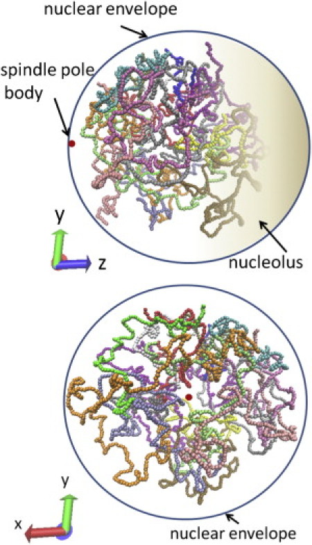
Snapshot of the simulated genome structure. Structures of 16 chromosomes are shown by different colors; Chr1 (blue), Chr2 (red), Chr3 (gray), Chr4 (orange), Chr5 (yellow), Chr6 (tan), Chr7 (silver), Chr8 (green), Chr9 (white), Chr10 (pink), Chr11 (cyan), Chr12 (purple), Chr13 (lime), Chr14 (mauve), Chr15 (ochre), and Chr16 (ice-blue). (Red dot) SPB. The shaded region is nucleolus. (Top) Snapshot drawn from the angle similar to that in Fig. 1. (Bottom) Same structure viewed from the SPB side. Simulated with ξ/T = 10 and Model 3.
After the equilibration process, each part of the genome continues to fluctuate largely. In Fig. 3, motions of centromeres (Fig. 3 a), distribution of rDNA (Fig. 3 b), and motions of telomeres (Fig. 3 c) and genes (Fig. 3 d) are shown. The trajectories of each gene and telomere traverse over one-half of the radius of nucleus, showing the large fluctuation of the genome structure. These trajectories, however, are not largely overlapped with each other. The amplitude of chromosome fluctuation is not large enough to homogenize nucleus completely, but parts of chromosomes are separated to form “territories” as has been pointed out by using the fluorescence data (17). (See also Movie S1 in the Supporting Material to grasp the feeling of the chromosome dynamics.)
Figure 3.
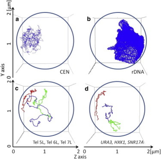
Examples of simulated trajectories of parts of the genome. (a) Trajectories of 16 centromeres are superposed. (b) Traces of the rDNA region moving during the simulation. (c) Trajectories of the left telomere of Chr5 (5L, blue); the left telomere of Chr6 (6L, red); and the left telomere of Chr7 (7L, green). (d) Trajectories of genes, ura3 (blue), hxk1 (red), and snr17a (green). The gene hxk1 is located near the telomere of Chr6, ura3 is near the centromere of Chr5, and snr17a is in between centromere and telomere of Chr15. Four spheres from panels a–d are viewed from the same angle: (a) Centromeres move around SPB. (b) rDNA spreads inside the nucleolus. (c) 6L moves near the nuclear envelope, 5L is bound and unbound to and from the nuclear envelope, and 7L moves more freely. (d) Genes move separately to form gene “territories”. Trajectories of 1.1 × 10⁵ steps simulated with ξ/T = 10 and Model 3 are shown.
Specific chromatin-chromatin interactions
We compare the results by varying the strength ξ of the Gō-like potential from ξ/T = 1 to 100. ξ/T represents the degree of how strongly the chromosome chains are constrained around their mean structures by the chromatin-chromatin interactions in the model. With ξ/T = 1, we can expect that the chromatin-chromatin interactions represented by the Gō-like potential are so weak that the other effects such as effects of fluctuating motions and constraints of the nuclear structure dominate dynamics of the system, whereas with ξ/T = 100 the chromatin-chromatin interactions dominate dynamics to give rise to a less flexible genome conformation.
Plotted in Fig. 4 are the observed (40) and simulated distributions of distances between telomeres. Each distribution has a large width showing the large amplitude motion of telomeres. The precise form of distribution, however, depends on the pair of telomeres examined, showing the heterogeneous fluctuations in the genome: Distance between the left telomere of Chr3 (3L) and the right telomere of Chr3 (3R) tends to be small, but the larger 6L-6R distance is observed and the 5L-5R and 14L-14R distances have further large variation.
Figure 4.
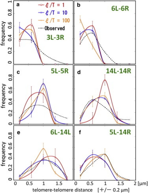
Dependence of telomere-telomere distance distributions on the strength of chromatin-chromatin interactions. Data simulated with ξ/T = 1 (red), ξ/T = 10 (blue), and ξ/T = 100 (orange) are compared with the data observed with the fluorescently labeled proteins (black dotted line) (40). Distributions between (a) 3L and 3R, (b) 6L and 6R, (c) 5L and 5R, (d) 14L and 14R, (e) 6L and 14L, and (f) 5L and 14R. Points obtained by binning data over ±0.2 μm are connected (smooth lines). (Error bars) Standard deviations of trajectories simulated for 5 × 10⁴ steps with Model 3.
The simulated results can semiquantitatively reproduce the observed data when the strength ξ is appropriately chosen: The distributions simulated with ξ/T = 10 can reasonably fit the experimental data for the 3L-3R, 6L-6R, 14L-14R, and 6L-14L distances, whereas the distribution simulated with ξ/T = 1 fails to fit the 14L-14R distance. The distribution simulated with ξ/T = 100 can fit the observed 5L-14R distance very well but fails to explain the 6L-6R distance. The 5L-5R distance cannot be fitted well by all the simulated results, which may be due to the limited sampling timesteps of trajectories. As shown in Fig. 3 c (and will be also shown in Fig. 6 a), 5L binds and unbinds to and from the nuclear envelope during the simulation, so that it should need the longer trajectories to sample enough data for the equilibrium distribution of the 5L-5R distance. Such large fluctuation of the position of 5L in the fluorescence data has been also reported (13).
Figure 6.
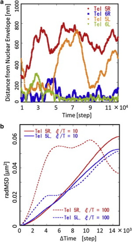
Simulated telomere dynamics. (a) Temporal change of the simulated distance between telomeres and the nuclear envelope is shown for 5R, 5L, 6R, and 6L. Simulated with ξ/T = 10 and Model 3. (b) msdR(t) of 5R and 5L are plotted as functions of the number of time steps t. Simulated data for ξ/T = 10 (lines) and 100 (dotted lines) with Model 3 are shown for 5L (blue) and 5R (red). By comparing the slope of simulated msdR(t) with the observed one (13), it is suggested that 11 × 104 steps in simulation roughly correspond to 290–490 s (see text for this estimation).
We should note that the Gō-like potential represents the consistency among the chromatin-chromatin interactions and other effects in nucleus and does not directly represent the physical interactions working through the formation of complexes of proteins that bind multiple chromosomes. The necessity of strong (ξ/T = 100) or moderately strong (ξ/T = 10) Gō-like potential for modeling the genome to reproduce the observed telomere-telomere distributions, however, strongly suggests that chromosomes are not the nonspecific polymer chains but the specific chromatin-chromatin interactions play important roles in organizing large but characteristic motions of chromosomes.
Heterogeneous interactions between chromosome and nuclear envelope
Also compared with the fluorescence data are four different models of attractive chromatin-envelope interactions represented by different distributions of {η(μ,i)}. Here, η(μ,i) is an index representing whether there is an attractive interaction between the ith site of the μth chain and the nuclear envelope (η = 1) or there is no such interaction between them (η = 0); Model 1 (η = 0 for all sites), Model 2 (η = 1 for all sites), Model 3 (η = 1 for telomere and rDNA sites, and η = 0 for other sites), and Model 4 (η = 1 for telomere and rDNA sites and sites near the nuclear envelope in the structure of Duan et al. (22), and η = 0 for other sites) were tested.
Because the regions of rDNA and the regions near telomeres are often found around the nuclear envelope in the fluorescence observations, the attractive interactions have been expected between rDNA and nuclear envelope (41) and also between telomeres and nuclear envelope (37). It is natural, therefore, that Model 1 does not explain the observed distributions (40) as shown in Fig. 5. In Fig. 5, we also find that Model 2 is inconsistent with the observed data, which implies that not every site but only the selected sites should form attractive protein complexes with the nuclear envelope.
Figure 5.
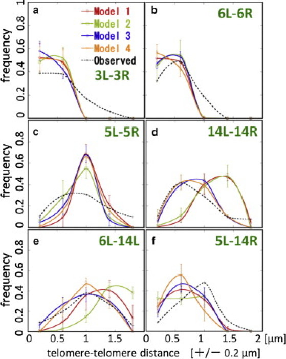
Dependence of telomere-telomere distance distributions on the interactions between chromatins and the nuclear envelope. Data simulated with Model 1 (red), Model 2 (green), Model 3 (blue), and Model 4 (orange) are compared with the data observed with the fluorescently labeled proteins (black dotted line) (40). Distributions between (a) 3L and 3R, (b) 6L and 6R, (c) 5L and 5R, (d) 14L and 14R, (e) 6L and 14L, and (f) 5L and 14R. Points obtained by binning data over ±0.2 μm are connected (smooth lines). (Error bars) Standard deviations of trajectories simulated for 5 × 10⁴ steps with ξ/T = 10.
Model 3 and Model 4 explain the observed data to a similar extent. Although Model 4 has the additional sites attractive to the nuclear envelope, the number of such sites is not large (11 sites in Chr1, 4 sites in Chr4, and 2 sites in Chr6), so that the effects are small in the resolution of Fig. 5. It would be interesting to further examine whether the more precise experimental measurement can distinguish the difference in distribution of {η(μ,i)}.
Diffusive movement of telomeres
Interesting features of the simulated data are the dynamical movement of chromosomes. Shown in Fig. 6 a is the distance between telomeres and the nuclear envelope. We can find that the telomere 5R is not bound to the nuclear envelope but 5L is transiently bound and unbound to and from the nuclear envelope. The telomeres 6R and 6L are bound to the nuclear envelope and distances between those sites and the nuclear envelope oscillate within a few hundred nanometers. These simulated features are consistent with the observed dynamical features of 5R, 5L, 6R, and 6L (13).
To compare the simulated data with the observed one, we define the radial mean-square displacement msdR of the site (μ,i) during the time steps t as
| (19) |
where 〈…〉τ is the average over τ for the trajectory examined. In Fig. 6 b, msdR(t) is plotted as a function of t. With this plot we can clearly see the difference between the results with ξ/T = 10 and those with ξ/T = 100: Fig. 6 b shows that msdR of 5L and 5R with ξ/T = 10 is roughly proportional to t, indicating that their motion is diffusive. With ξ/T = 100, on the other hand, msdR shows a complex pattern with the oscillatory behaviors, which indicates the elastic features of the genome structure arising from the strong chromatin-chromatin interactions. The experimental data show that msdR is diffusive without exhibiting an oscillatory behavior (13). We should conclude, therefore, that in yeast genome the constraints due to the chromatin-chromatin interactions are not so strong as to generate the elastic stiffness but are at the moderate level to keep fluidity of the genome structure in nucleus. By comparing the slope of msdR(t) for ξ/T = 10 with the experimental data (13), the suggested length of a step in the simulation is 2.63 × 10⁻³ s/step when the 5L data are used and 4.47 × 10⁻³ s/step when the 5R data are used. With this estimation of order of timescale, the length of trajectories shown in Fig. 6 a corresponds to ∼290–490 s.
Discussion
In this article a method was developed for modeling dynamical three-dimensional organization of genome of interphase budding yeast. The modeled genome exhibits a large structural fluctuation with the diffusive motion of chromosomes. Despite such intense fluctuation, the simulated movement of chromosomes is not completely random but is subjected to both the specific chromatin-chromatin interactions and the heterogeneous chromatin-envelope interactions: By suitably taking into account the information obtained from the 3C-based method, the model explained the fluorescence data for the distribution and movement of each part of the genome.
We should note that an important point to be improved in the present modeling is on the treatment of nucleolus. In our model, nucleolus was considered as a force field acting on chromosomes. Nucleolus, however, is a complex of ribosomal DNA, RNA, and related proteins, and should behave as a deformable substance. Moving chromosomes should push the nucleolus to deform it to a concave form and the deformed nucleolus should then apply forces on chromosomes in a different way from that considered in our model. By treating nucleolus in a more realistic way, we may be able to construct a model that should have more quantitative prediction capability.
With such improvement, we will be able to explore many challenging problems. For example, genes actively transcribed may be anchored around the nuclear pore (3, 38). The attractive interaction between the gene at site (μ,i) and the nuclear envelope is represented by η(μ,i) in our model, so that the model may predict how the gene expression pattern and the observation on the movement of that gene is correlated. Another interesting problem is on the distribution of the protein factors involved in the complex to anchor chromosomes to the nuclear envelope. Because the formation of complexes may bring about the sequestration of such factors, the model may predict the spatiotemporal pattern of confinement and release of those factors. Also interesting is the dynamical movement of chromosomes. We may analyze it, for example, by decomposing the movement into principal components. It would be intriguing to see whether there is a correlation between those components and principal modes of the temporal variation of gene expression.
It is also interesting to see the effects of heterogeneous rigidity of the chromosome chains. It has been shown that the loci of induced DSB are dislocated to the nuclear periphery to form the repair domain (42, 43). The localized modulation of stiffness parameters such as k in Eq. 6 or kϕ in Eq. 8 should represent DSB at the corresponding loci in the model, and hence it should be possible to examine whether the DSB loci move owing to interactions mediated by specific proteins or through the biased diffusion in the organized genome structure.
In this way the efforts to construct the computational model of dynamical three-dimensional genome organization should lead to a unified view of the genome structure, dynamics, and function, so that it should open a new field of interacting computational and experimental biophysics of structural genetics.
Acknowledgments
This work was partially supported by Grants-in-Aid for Scientific Research from Japan Society for the Promotion of Science.
Editor: Laura Finzi.
Footnotes
One movie is available at http://www.biophysj.org/biophysj/supplemental/S0006-3495(11)05401-4.
Supporting Material
References
- 1.Misteli T. Beyond the sequence: cellular organization of genome function. Cell. 2007;128:787–800. doi: 10.1016/j.cell.2007.01.028. [DOI] [PubMed] [Google Scholar]
- 2.Miele A., Dekker J. Long-range chromosomal interactions and gene regulation. Mol. Biosyst. 2008;4:1046–1057. doi: 10.1039/b803580f. [DOI] [PMC free article] [PubMed] [Google Scholar]
- 3.Dillon N. The impact of gene location in the nucleus on transcriptional regulation. Dev. Cell. 2008;15:182–186. doi: 10.1016/j.devcel.2008.07.013. [DOI] [PubMed] [Google Scholar]
- 4.Zimmer C., Fabre E. Principles of chromosomal organization: lessons from yeast. J. Cell Biol. 2011;192:723–733. doi: 10.1083/jcb.201010058. [DOI] [PMC free article] [PubMed] [Google Scholar]
- 5.Lanctôt C., Cheutin T., et al. Cremer T. Dynamic genome architecture in the nuclear space: regulation of gene expression in three dimensions. Nat. Rev. Genet. 2007;8:104–115. doi: 10.1038/nrg2041. [DOI] [PubMed] [Google Scholar]
- 6.Lieberman-Aiden E., van Berkum N.L., et al. Dekker J. Comprehensive mapping of long-range interactions reveals folding principles of the human genome. Science. 2009;326:289–293. doi: 10.1126/science.1181369. [DOI] [PMC free article] [PubMed] [Google Scholar]
- 7.Grosberg A., Rabin Y., et al. Neer A. Crumpled globule model of the three-dimensional structure of DNA. Europhys. Lett. 1993;23:373–378. [Google Scholar]
- 8.Mirny L.A. The fractal globule as a model of chromatin architecture in the cell. Chromosome Res. 2011;19:37–51. doi: 10.1007/s10577-010-9177-0. [DOI] [PMC free article] [PubMed] [Google Scholar]
- 9.Rosa A., Everaers R. Structure and dynamics of interphase chromosomes. PLoS Comput. Biol. 2008;4:e1000153. doi: 10.1371/journal.pcbi.1000153. [DOI] [PMC free article] [PubMed] [Google Scholar]
- 10.Rosa A., Becker N.B., Everaers R. Looping probabilities in model interphase chromosomes. Biophys. J. 2010;98:2410–2419. doi: 10.1016/j.bpj.2010.01.054. [DOI] [PMC free article] [PubMed] [Google Scholar]
- 11.Heun P., Laroche T., et al. Gasser S.M. Chromosome dynamics in the yeast interphase nucleus. Science. 2001;294:2181–2186. doi: 10.1126/science.1065366. [DOI] [PubMed] [Google Scholar]
- 12.Gasser S.M. Visualizing chromatin dynamics in interphase nuclei. Science. 2002;296:1412–1416. doi: 10.1126/science.1067703. [DOI] [PubMed] [Google Scholar]
- 13.Hediger F., Neumann F.R., et al. Gasser S.M. Live imaging of telomeres: yKu and Sir proteins define redundant telomere-anchoring pathways in yeast. Curr. Biol. 2002;12:2076–2089. doi: 10.1016/s0960-9822(02)01338-6. [DOI] [PubMed] [Google Scholar]
- 14.Schober H., Kalck V., et al. Gasser S.M. Controlled exchange of chromosomal arms reveals principles driving telomere interactions in yeast. Genome Res. 2008;18:261–271. doi: 10.1101/gr.6687808. [DOI] [PMC free article] [PubMed] [Google Scholar]
- 15.Therizols P., Duong T., et al. Fabre E. Chromosome arm length and nuclear constraints determine the dynamic relationship of yeast subtelomeres. Proc. Natl. Acad. Sci. USA. 2010;107:2025–2030. doi: 10.1073/pnas.0914187107. [DOI] [PMC free article] [PubMed] [Google Scholar]
- 16.Maeshima K., Hihara S., Eltsov M. Chromatin structure: does the 30-nm fiber exist in vivo? Curr. Opin. Cell Biol. 2010;22:291–297. doi: 10.1016/j.ceb.2010.03.001. [DOI] [PubMed] [Google Scholar]
- 17.Berger A.B., Cabal G.G., et al. Zimmer C. High-resolution statistical mapping reveals gene territories in live yeast. Nat. Methods. 2008;5:1031–1037. doi: 10.1038/nmeth.1266. [DOI] [PubMed] [Google Scholar]
- 18.Ferrai C., de Castro I.J., et al. Pombo A. Gene positioning. Cold Spring Harb. Perspect. Biol. 2010;2:a000588. doi: 10.1101/cshperspect.a000588. [DOI] [PMC free article] [PubMed] [Google Scholar]
- 19.Bystricky K., Heun P., et al. Gasser S.M. Long-range compaction and flexibility of interphase chromatin in budding yeast analyzed by high-resolution imaging techniques. Proc. Natl. Acad. Sci. USA. 2004;101:16495–16500. doi: 10.1073/pnas.0402766101. [DOI] [PMC free article] [PubMed] [Google Scholar]
- 20.Taddei A., Schober H., Gasser S.M. The budding yeast nucleus. Cold Spring Harb. Perspect. Biol. 2010;2:a000612. doi: 10.1101/cshperspect.a000612. [DOI] [PMC free article] [PubMed] [Google Scholar]
- 21.Torres-Rosell J., Sunjevaric I., et al. Lisby M. The Smc5-Smc6 complex and SUMO modification of Rad52 regulates recombinational repair at the ribosomal gene locus. Nat. Cell Biol. 2007;9:923–931. doi: 10.1038/ncb1619. [DOI] [PubMed] [Google Scholar]
- 22.Duan Z., Andronescu M., et al. Noble W.S. A three-dimensional model of the yeast genome. Nature. 2010;465:363–367. doi: 10.1038/nature08973. [DOI] [PMC free article] [PubMed] [Google Scholar]
- 23.Tanizawa H., Iwasaki O., et al. Noma K. Mapping of long-range associations throughout the fission yeast genome reveals global genome organization linked to transcriptional regulation. Nucleic Acids Res. 2010;38:8164–8177. doi: 10.1093/nar/gkq955. [DOI] [PMC free article] [PubMed] [Google Scholar]
- 24.Lisby M., Mortensen U.H., Rothstein R. Colocalization of multiple DNA double-strand breaks at a single Rad52 repair centre. Nat. Cell Biol. 2003;5:572–577. doi: 10.1038/ncb997. [DOI] [PubMed] [Google Scholar]
- 25.Marti-Renom M.A., Mirny L.A. Bridging the resolution gap in structural modeling of 3D genome organization. PLoS Comput. Biol. 2011;7:e1002125. doi: 10.1371/journal.pcbi.1002125. [DOI] [PMC free article] [PubMed] [Google Scholar]
- 26.Onuchic J.N., Wolynes P.G. Theory of protein folding. Curr. Opin. Struct. Biol. 2004;14:70–75. doi: 10.1016/j.sbi.2004.01.009. [DOI] [PubMed] [Google Scholar]
- 27.Taketomi H., Ueda Y., Gō N. Studies on protein folding, unfolding and fluctuations by computer simulation. I. The effect of specific amino acid sequence represented by specific inter-unit interactions. Int. J. Pept. Protein Res. 1975;7:445–459. [PubMed] [Google Scholar]
- 28.Clementi C., Nymeyer H., Onuchic J.N. Topological and energetic factors: what determines the structural details of the transition state ensemble and “en-route” intermediates for protein folding? An investigation for small globular proteins. J. Mol. Biol. 2000;298:937–953. doi: 10.1006/jmbi.2000.3693. [DOI] [PubMed] [Google Scholar]
- 29.Kremer K., Grest G.S. Dynamics of entangled linear polymer melts: a molecular-dynamics simulation. J. Chem. Phys. 1990;92:5057–5086. [Google Scholar]
- 30.Worcel A., Strogatz S., Riley D. Structure of chromatin and the linking number of DNA. Proc. Natl. Acad. Sci. USA. 1981;78:1461–1465. doi: 10.1073/pnas.78.3.1461. [DOI] [PMC free article] [PubMed] [Google Scholar]
- 31.Lankas F., Lavery R., Maddocks J.H. Kinking occurs during molecular dynamics simulations of small DNA minicircles. Structure. 2006;14:1527–1534. doi: 10.1016/j.str.2006.08.004. [DOI] [PubMed] [Google Scholar]
- 32.Wiggins P.A., Phillips R., Nelson P.C. Exact theory of kinkable elastic polymers. Phys. Rev. E. 2005;71:021909. doi: 10.1103/PhysRevE.71.021909. [DOI] [PMC free article] [PubMed] [Google Scholar]
- 33.Hagerman P.J. Flexibility of DNA. Annu. Rev. Biophys. Biophys. Chem. 1988;17:265–286. doi: 10.1146/annurev.bb.17.060188.001405. [DOI] [PubMed] [Google Scholar]
- 34.Goldstein R.A., Luthey-Schulten Z.A., Wolynes P.G. Optimal protein-folding codes from spin-glass theory. Proc. Natl. Acad. Sci. USA. 1992;89:4918–4922. doi: 10.1073/pnas.89.11.4918. [DOI] [PMC free article] [PubMed] [Google Scholar]
- 35.Sasai M. Conformation, energy, and folding ability of selected amino acid sequences. Proc. Natl. Acad. Sci. USA. 1995;92:8438–8442. doi: 10.1073/pnas.92.18.8438. [DOI] [PMC free article] [PubMed] [Google Scholar]
- 36.Sasaki T.N., Cetin H., Sasai M. A coarse-grained Langevin molecular dynamics approach to de novo protein structure prediction. Biochem. Biophys. Res. Commun. 2008;369:500–506. doi: 10.1016/j.bbrc.2008.02.048. [DOI] [PubMed] [Google Scholar]
- 37.Taddei A., Van Houwe G., et al. Gasser S.M. The functional importance of telomere clustering: global changes in gene expression result from SIR factor dispersion. Genome Res. 2009;19:611–625. doi: 10.1101/gr.083881.108. [DOI] [PMC free article] [PubMed] [Google Scholar]
- 38.Taddei A., Van Houwe G., et al. Gasser S.M. Nuclear pore association confers optimal expression levels for an inducible yeast gene. Nature. 2006;441:774–778. doi: 10.1038/nature04845. [DOI] [PubMed] [Google Scholar]
- 39.Saccharomyces Genome Database. http://www.yeastgenome.org/
- 40.Bystricky K., Laroche T., et al. Gasser S.M. Chromosome looping in yeast: telomere pairing and coordinated movement reflect anchoring efficiency and territorial organization. J. Cell Biol. 2005;168:375–387. doi: 10.1083/jcb.200409091. [DOI] [PMC free article] [PubMed] [Google Scholar]
- 41.Mekhail K., Seebacher J., et al. Moazed D. Role for perinuclear chromosome tethering in maintenance of genome stability. Nature. 2008;456:667–670. doi: 10.1038/nature07460. [DOI] [PMC free article] [PubMed] [Google Scholar]
- 42.Therizols P., Fairhead C., et al. Fabre E. Telomere tethering at the nuclear periphery is essential for efficient DNA double strand break repair in subtelomeric region. J. Cell Biol. 2006;172:189–199. doi: 10.1083/jcb.200505159. [DOI] [PMC free article] [PubMed] [Google Scholar]
- 43.Nagai S., Dubrana K., et al. Krogan N.J. Functional targeting of DNA damage to a nuclear pore-associated SUMO-dependent ubiquitin ligase. Science. 2008;322:597–602. doi: 10.1126/science.1162790. [DOI] [PMC free article] [PubMed] [Google Scholar]
Associated Data
This section collects any data citations, data availability statements, or supplementary materials included in this article.