

Abstract
The question of which statistical approach is the most effective for investigating gene-environment (G-E) interactions in the context of genome-wide association studies (GWAS) remains unresolved. By using 2 case-control GWAS (the Nurses’ Health Study, 1976–2006, and the Health Professionals Follow-up Study, 1986–2006) of type 2 diabetes, the authors compared 5 tests for interactions: standard logistic regression-based case-control; case-only; semiparametric maximum-likelihood estimation of an empirical-Bayes shrinkage estimator; and 2-stage tests. The authors also compared 2 joint tests of genetic main effects and G-E interaction. Elevated body mass index was the exposure of interest and was modeled as a binary trait to avoid an inflated type I error rate that the authors observed when the main effect of continuous body mass index was misspecified. Although both the case-only and the semiparametric maximum-likelihood estimation approaches assume that the tested markers are independent of exposure in the general population, the authors did not observe any evidence of inflated type I error for these tests in their studies with 2,199 cases and 3,044 controls. Both joint tests detected markers with known marginal effects. Loci with the most significant G-E interactions using the standard, empirical-Bayes, and 2-stage tests were strongly correlated with the exposure among controls. Study findings suggest that methods exploiting G-E independence can be efficient and valid options for investigating G-E interactions in GWAS.
Keywords: case-control studies; case study; diabetes mellitus, type 2; epidemiologic methods; genome-wide association study; genotype-environment interaction
Genome-wide association studies (GWAS) have contributed substantially to our understanding of the genetic underpinnings of various complex diseases. However, nearly all GWAS to date have focused on characterizing marginal genetic effects and have not fully explored the potential role environmental factors play in modifying genetic risk. Despite the growing enthusiasm for investigation of gene-environment (G-E) interactions, the most effective way to apply and detect interactions in the context of GWAS remains unresolved (1).
The standard logistic regression test for G-E interactions (defined as departure from a multiplicative odds ratio model; refer to the Appendix) remains an established method to analyze case-control data but is generally underpowered to detect G-E interactions unless the genetic and environmental factors are common and the interaction is strong (2). More powerful methods to detect G-E interactions, such as the case-only approach, rely on the assumption that genetic and environmental factors are independent in the source population, but these tests are subject to inflated type I error when the assumption is violated (3–6). Recently proposed hybrid or “hedge” methodologies seek to leverage the potential efficiency gains of the case-only method with the robustness property of the standard case-control approach (7, 8).
Some argue that G-E interactions might be used to enhance detection of genes that are potentially missed by conventional GWAS. Joint tests of both the genetic main effects and G-E interactions have been developed for this purpose (9). Exploratory approaches, such as multifactor dimensionality reduction and tree-based and other data-mining methods, have also been proposed for testing G-E interactions but are currently computationally intensive, and their performance and interpretation in the context of genome-wide level data are unclear (10–14).
Logistic regression-based tests for G-E interactions have been evaluated primarily by simulation and small-scale multimarker studies, and little is known on how they perform on empirical genome-wide level data (15). In this paper, we provide a comparative study of several logistic regression-based tests of G-E interactions in a real GWAS setting. The GWAS approach has been especially successful in identifying novel variants underlying type 2 diabetes (16). It is well known, however, that type 2 diabetes is a result of a combination of genetic and environmental factors (17). An adipogenic environment, usually marked by an elevated body mass index, is a particularly strong risk factor that may interact in a statistical sense with a genetic propensity for the disease (although the biologic implications of such an interaction are not immediately clear) (18–21). Body mass index is partially under genetic control (22, 23), violating a key assumption of several of the statistical methods we examine. Thus, our investigation of gene-body mass index interactions in type 2 diabetes provides an interesting empirical comparison of the performance of several approaches to the analysis of G-E interactions in terms of their type I and II errors and their robustness to violations of the gene-environment independence assumption.
MATERIALS AND METHODS
Statistical tests
We evaluate the performance of 2 classes of statistical tests: a 1 df test of G-E interaction (defined as departure from a multiplicative odds ratio model; refer to the Appendix) and a 2 df test of genetic main effect and G-E interaction. The 1 df class includes the standard logistic regression-based case-control, case-only, and semiparametric maximum-likelihood estimation (semi-MLE) tests, as well as 2 “hedge” methods: an empirical-Bayes shrinkage estimator and a 2-stage test (3, 4, 7, 8, 24). These 2 classes test distinct null hypotheses: The 1 df statistics test the null hypothesis of no G-E interaction per se, while the 2-df statistics test the null hypothesis that the genetic marker under study is not associated with disease, in any stratum defined by exposure. Which class of test is more appropriate will depend on the aims of the study. If investigators are interested in detecting departures from a multiplicative odds ratio model (e.g., when studying markers with known marginal associations with disease), then the 2 df test will be confounded by the genetic main effect; on the other hand, if investigators are interested in discovering new markers, leveraging potential G-E interactions, then the 2 df test is often much more powerful than the 1 df test (9, 25). In the Appendix, we describe the statistical details of all 7 tests. We limit our discussion of G-E interaction to departures from a multiplicative odds ratio model, although other forms of interaction can be tested by using case-control data (26–28). (The case-only method can only be used to test departures from a multiplicative model (3)). We consider these tests in the context of gene discovery, where the goal is to identify markers that have not been identified by an initial screen of marginal genetic effects.
Genome-wide G-E interaction studies of type 2 diabetes
We apply these 7 statistical tests to 2 nested case-control type 2 diabetes GWAS in the Nurses’ Health Study (NHS) and the Health Professionals Follow-up Study (HPFS) cohorts. Details regarding the study design including population, data collection, genotyping quality control, and assurance have been reported elsewhere (29, 30). All participants provided written informed consent, and the study was approved by the Institutional Review Board of the Brigham and Women’s Hospital and the Human Subjects Committee Review Board of the Harvard School of Public Health. The original analysis of marginal, single-marker effects included 3,221 women (NHS) and 2,422 men (HPFS) of genetically inferred European ancestry. Quantile-quantile plots for both studies did not suggest any large-scale systematic bias due to population stratification or differential genotyping error (29). We restricted the current analysis to incident cases of type 2 diabetes, because reliable body mass index measures prior to diagnosis were not available for prevalent cases. Body mass index was self-reported and calculated as follows: weight (kg)/height (m)2 (31). Self-administered questionnaires about body weight have been validated as described previously (31). The final sample included 3,072 (1,321 cases and 1,751 controls) for NHS and 2,171 (878 cases and 1,293 controls) for HPFS with genome-wide scans and information on body mass index. The current analysis was restricted to single nucleotide polymorphisms (SNPs) mapped to chromosomes 1 through 22, as annotated on the Affy 6.0 chip (Affymetrix, Santa Clara, California), leaving a total of 678,082 quality SNPs in the NHS data set and 678,540 SNPs in the HPFS data set.
For all 7 methods, we assumed a log additive mode of inheritance for each SNP in the interaction model; that is, G was coded as a count of minor alleles for each SNP. Body mass index was modeled as a binary trait to guard against inflated type I error in tests of interaction when the main effect of environment is misspecified (refer to Results). We defined a “high” body mass index as ≥25 kg/m2 in 1976 (baseline) for women and ≥30 kg/m2 in 1986 (baseline) for men. The different cutpoints used for each cohort reflect cohort differences in body mass index distribution at baseline. Analysis proceeded without adjustment for covariates. In order to achieve more precise estimators of parameters when applying the semiparametric maximum-likelihood estimation test (4), we constrained the probability of disease as determined for each cohort to 0.084 in the NHS and 0.068 in the HPFS. We note that this test can be implemented in a more general setting that does not require specifying baseline disease probabilities. The maximum-likelihood estimates were obtained for all unknown parameters. For the 2-stage approach, we applied an α1 = 0.01 at the first stage, which has been shown to perform well in simulation studies (7) (although more recent work suggests that other thresholds can lead to greater power (32)). For comparison purposes, second-stage P values for the 2-stage test were multiplied by 0.01 to account for the fewer statistical tests performed relative to the other 1 df tests.
Analyses were conducted by using PLINK (33) and the SAS, version 9.1 for UNIX, statistical package (SAS Institute, Inc., Cary, North Carolina). R was used for graphical presentation (www.r-project.org). Although the current study was restricted to genotyped SNPs, all tests under consideration can be applied to a setting where imputed SNPs are examined. Quantile-quantile plots that display the empirical percentile of the interaction test P values against the percentiles of the expected null distribution were used to compare type 1 error rates across the different interaction tests. To complement our empirical analyses, we also present the theoretical type I error rate for these tests calculated under different assumptions regarding the strength of the G-E correlation and the fraction of markers correlated with E (refer to the Appendix) (34).
RESULTS
Characteristics of the NHS and HPFS data sets are presented in Web Table 1 (the first of 4 Web tables and 8 Web figures posted on the Journal’s Web site (http://aje.oupjournals.org/)). Body mass index was strongly associated with type 2 diabetes: Compared with a low body mass index, the odds ratio of type 2 diabetes associated with a high body mass index was 4.73 (95% confidence interval (CI): 4.05, 5.52) for women and 6.91 (95% CI: 5.18, 9.23) for men.
We first considered the impact of potentially misspecifying the main effect of E (body mass index) in the standard G-E interaction tests using the NHS data set. Each plot in Figure 1 displays the empirical percentile of the interaction test P values corresponding to 1 of 4 approaches to modeling body mass index against the percentiles of the expected null distribution. When body mass index is modeled as a linear continuous variable, we observe a dramatic departure from the diagonal line at P < 0.01, indicative of systemic inflation of the type I error rate (λ = 1.47; Figure 1, model 1). Similar results were observed for the joint 2 df test and when analyses were conducted by using the HPFS data set (data not shown). The standard case-only test, which does not make any assumptions about the functional form of the environmental main effect (although it implicitly assumes a functional form for the G-E interaction effect by regressing E on G among cases; refer to the Appendix), was not subject to this inflation when body mass index was modeled as a linear continuous variable (λ = 1.00) (Web Figure 1).
Figure 1.

Quantile-quantile plots for approaches to modeling body mass index in the standard gene-environment (G-E) interaction test: 1) model 1: logit Pr(D|G,E) = β0 + βg G + βe E + βge G × E, where E (body mass index) is a continuous variable (○); 2) model 2: logit Pr(D|G,E) = β0 + βg G + βe1 E + βe2 E2 + βe3 E3 + βge G × E, where E (modeled as body mass index − mean) is a continuous variable (▵); 3) model 3: model 1 with robust variance estimator (*); and 4) model 4: logit Pr(D|G,E) = β0 + βg G + βe E + βge G × E, where E (body mass index) is a binary variable (+), in the Nurses’ Health Study, 1976–2006. The dashed line (y = x line) corresponds to instances where the observed (y) P value is equal to the expected (x) P value.
This inflation results from model misspecification under the null, which causes the variance of βge to be underestimated, leading to inflated test statistics (35). There are at least 3 solutions to this problem. 1) A more flexible model for the environmental main effect could be used. In our case, adding a quadratic and cubic body mass index term to the model removed the inflation in the quantile-quantile plot (λ = 1.47 for linear body mass index, λ = 1.04 for polynomial body mass index) (Figure 1, model 2). We note that, even if a more complicated form for the main effect of exposure is used, including a simple G- (linear E) term in the model still leads to a valid test of interaction (βge = 0), although the single interaction parameter may not capture the full complexity of the interaction pattern. 2) A robust “sandwich” estimator of the variance could be used (λ = 1.02; Figure 1, model 3). 3) A continuous exposure could be modeled by using general categorical variables (e.g., dichotomizing the exposure (λ = 1.01; Figure 1, model 4) or assigning each subject to distinct low, medium, or high exposure categories and using 2 indicator variables for the nonreference group. Although this last approach can result in the loss of some information, it allows a saturated model to be used for the environmental main effect, which eliminates the problem of model misspecification under the null. As in the previous 2 approaches, the saturated model for the G-E interaction is not necessary for validity. This is the approach that we took in all the subsequent analyses: We used a simple binary environmental exposure for purposes of comparing these 7 tests.
Because of space constraints, we present and focus our attention on results from the NHS data set and place all equivalent tables and figures for HPFS analysis online (Web Table 2; Web Figures 2–4). Unless noted otherwise, the qualitative pattern of test performance was similar in the NHS and the HPFS data sets. With only 1 exception (10q25: TCF7L2), however, none of the top (P < 1 × 10⁻⁵) G-E interactions (1 df) or loci (2 df) overlapped between the 2 data sets.
Figure 2 displays the quantile-quantile plots for the 1 df tests for interaction with a color-coding scheme corresponding to logistic regression tests for G-E association among controls. None of these tests shows evidence for systematic inflation in type I error rates (λ ≤ 1.008) or any individual genome-wide significant G-E interaction. The test statistics for the empirical-Bayes hedge method are all slightly smaller than their asymptotic null distribution (λ = 0.936), suggesting that in these samples sizes the asymptotic approximation does not hold (8). For each test, Table 1 presents detailed results for G-E interactions with P < 1 × 10⁻⁵ and how these results compare across the other tests for interaction. With few exceptions, all the top G-E interactions for the standard test (P < 1 × 10⁻⁵) demonstrate highly significant G-E dependence, with G-E effect estimates in an opposite direction to that of the interaction. A similar, but less dramatic, pattern was observed for the 2 hedge methods. These G-E interactions were scattered across the genome, and thus the enrichment for G-E dependence was not driven by a set of SNPs in high linkage disequilibrium. In contrast, for the case-only and semiparametric maximum-likelihood estimation tests, the strongest G-E interactions showed no evidence of G-E dependence. As shown in the genome-wide test correlation matrix (Web Figure 5), the strongest correlations among test P values were observed between the case-only and the semiparametric maximum-likelihood estimation tests (r = 0.96), while the weakest correlation occurred between the standard and case-only tests (r = 0.38).
Figure 2.

Quantile-quantile plots and corresponding genomic inflation factors (lambda) for the 1 df tests for gene-environment (G-E) interaction (standard case-control (A), case-only (B), semiparametric maximum-likelihood estimation (C), empirical-Bayes shrinkage estimator (D), and 2-stage (E)) in the Nurses’ Health Study, 1976–2006. Point colors correspond to P values for tests of G-E dependence: <0.001 (black), <0.05 (gray), and ≥0.05 (white). For the 2-stage test (E), lambda was calculated by using P values from 7,231 single nucleotide polymorphisms tested in the second stage. The dashed line (y = x line) corresponds to instances where the observed (y) P value is equal to the expected (x) P value.
Table 1.
Cross-Test Comparison of Nominally Significant (P < 1 × 10⁻⁵) G-E Interactions Detected by Each of the 1 df Tests in the Nurses’ Health Study, 1976–2006
| SNP | Region | No. of SNPs in LDa | MAF (“risk”) for Cases | MAF (“risk”) for Controls |
G-E Association |
Marginal G Effect |
Tests for G-E Interaction |
|||||||||||
| Standard |
Case-Only |
2-Stage |
EB Shrinkage |
Semi-MLE |
||||||||||||||
| β Co-efficient | P Value | β Co-efficient | P Value | β Co-efficient | P Value | β Co-efficient | P Value | β Co-efficient | P Value | β Co-efficient | P Value | β Co-efficient | P Value | |||||
| Standard | ||||||||||||||||||
| rs2110169 | 12p13 | 0 | 0.37 | 0.39 | 0.34 | 2.2 × 10⁻⁵ | −0.103 | 0.06 | −0.55 | 2.4 × 10⁻⁶ | −0.20 | 0.018 | −0.51 | 2.0 × 10⁻⁵ | −0.28 | 0.0022 | ||
| rs10512802 | 3q21 | 0 | 0.03 | 0.03 | 0.88 | 6.6 × 10⁻⁵ | 0.037 | 0.82 | −1.52 | 4.1 × 10⁻⁶ | −0.64 | 0.0089 | −1.41 | 4.0 × 10⁻⁵ | −0.84 | 0.0020 | ||
| rs9992452 | 4q35 | 0 | 0.16 | 0.15 | 0.44 | 2.5 × 10⁻⁵ | 0.030 | 0.67 | −0.68 | 6.5 × 10⁻⁶ | −0.25 | 0.025 | −0.63 | 5.4 × 10⁻⁵ | −0.33 | 0.0067 | ||
| rs11669653 | 19q13.1 | 0 | 0.30 | 0.30 | 0.23 | 0.0058 | 0.002 | 0.97 | −0.54 | 8.7 × 10⁻⁶ | −0.31 | 0.00041 | −0.49 | 1.4 × 10⁻⁴ | −0.36 | 0.00015 | ||
| Case-only | ||||||||||||||||||
| rs7687423 | 4q32 | 0 | 0.37 | 0.40 | 0.04 | 0.57 | −0.14 | 0.0071 | −0.43 | 1.4 × 10⁻⁴ | −0.40 | 1.9 × 10⁻⁶ | −0.43 | 1.4 × 10⁻⁶ | −0.40 | 4.7 × 10⁻⁶ | −0.45 | 6.7 × 10⁻⁷ |
| rs12488683 | 3q22 | 0 | 0.34 | 0.33 | −0.05 | 0.59 | 0.032 | 0.56 | −0.35 | 0.0043 | −0.40 | 5.7 × 10⁻⁶ | −0.35 | 4.3 × 10⁻⁵ | −0.39 | 2.1 × 10⁻⁵ | −0.41 | 1.7 × 10⁻⁵ |
| rs6818789 | 4q35 | 0 | 0.11 | 0.11 | 0.13 | 0.29 | −0.027 | 0.75 | 0.50 | 0.0071 | 0.64 | 8.6 × 10⁻⁶ | 0.50 | 7.1 × 10⁻⁵ | 0.59 | 4.4 × 10⁻⁴ | 0.65 | 2.1 × 10⁻⁵ |
| 2-Stage | ||||||||||||||||||
| rs2883160 | 1q43 | 1 | 0.25 | 0.24 | 0.42 | 1.7 × 10⁻⁶ | 0.033 | 0.58 | −0.51 | 9.0 × 10⁻⁵ | −0.08 | 0.41 | −0.51 | 9.0 × 10⁻⁷ | −0.47 | 4.7 × 10⁻⁴ | −0.14 | 0.17 |
| rs7687423 | 4q32 | 1 | 0.37 | 0.40 | 0.04 | 0.57 | −0.141 | 0.0071 | −0.43 | 1.4 × 10⁻⁴ | −0.40 | 1.9 × 10⁻⁶ | −0.43 | 1.4 × 10⁻⁶ | −0.40 | 4.7 × 10⁻⁶ | −0.45 | 6.7 × 10⁻⁷ |
| rs2248178 | 8q22 | 1 | 0.15 | 0.14 | 0.47 | 9.5 × 10⁻⁶ | 0.073 | 0.31 | −0.54 | 4.4 × 10⁻⁴ | −0.08 | 0.47 | −0.54 | 4.4 × 10⁻⁶ | −0.49 | 0.0019 | −0.15 | 0.22 |
| rs879993 | 12q24.3 | 0 | 0.13 | 0.12 | −0.10 | 0.42 | 0.096 | 0.22 | 0.63 | 4.8 × 10⁻⁴ | 0.52 | 5.5 × 10⁻⁵ | 0.63 | 4.8 × 10⁻⁶ | 0.55 | 2.5 × 10⁻⁴ | 0.60 | 2.7 × 10⁻⁵ |
| rs10459511 | 14q22 | 0 | 0.07 | 0.08 | −0.64 | 1.6 × 10⁻⁴ | −0.178 | 0.076 | 0.78 | 9.2 × 10⁻⁴ | 0.14 | 0.40 | 0.78 | 9.2 × 10⁻⁶ | 0.70 | 0.0044 | 0.20 | 0.26 |
| EB Shrinkage | ||||||||||||||||||
| rs7687423 | 4q32 | 0 | 0.37 | 0.40 | 0.04 | 0.57 | −0.14 | 0.0071 | −0.43 | 1.4 × 10⁻⁴ | −0.40 | 1.9 × 10⁻⁶ | −0.43 | 1.4 × 10⁻⁶ | −0.40 | 4.7 × 10⁻⁶ | −0.45 | 6.7 × 10⁻⁷ |
| Semi-MLE | ||||||||||||||||||
| rs7687423 | 4q32 | 0 | 0.37 | 0.40 | 0.04 | 0.57 | −0.14 | 0.0071 | −0.43 | 1.4 × 10⁻⁴ | −0.40 | 1.9 × 10⁻⁶ | −0.43 | 1.4 × 10⁻⁶ | −0.40 | 4.7 × 10⁻⁶ | −0.45 | 6.7 × 10⁻⁷ |
Abbreviations: EB, empirical-Bayes; G, gene; G-E, gene-environment; LD, linkage disequilibrium; MAF, minor allele frequency; semi-MLE, semiparametric maximum-likelihood estimation; SNP, single nucleotide polymorphism.
Number of SNPs in linkage disequilibrium (r2 > 0.8) with P < 1 × 10⁻⁵ for the G-E interaction test.
Figure 3 displays quantile-quantile plots for the joint 2 df test and semiparametric maximum-likelihood estimation 2 df test. For comparison purposes, we also present results from the case-control test for marginal genetic effects, adjusted and unadjusted for body mass index. The marginal effects test adjusted for body mass index and both 2 df tests detected strong signals missed by the unadjusted marginal effects test (Table 2). Of special note, the cluster of SNPs in region 10q25 are significantly associated with type 2 diabetes on the basis of the adjusted marginal effects test and joint tests (P < 1 × 10⁻⁶), but they are not significantly associated with the disease according to the unadjusted marginal genetic effect test. This region maps to TCF7L2, an established risk locus for type 2 diabetes (36). Applying the 2 df tests to the HPFS data set did not reveal any additional loci (P < 1 × 10⁻⁵) but did, however, capture all risk loci identified by the marginal effects test (Web Table 3). Results from all 3 tests were strongly correlated in both the NHS (r > 0.53; Web Figure 6) and the HPFS (r > 0.56) (Web Figure 7).
Figure 3.

Quantile-quantile plots and corresponding genomic inflation factors (lambda) for the marginal genetic effects test (unadjusted (A) and adjusted (B) for body mass index) and for joint tests of genetic main effects and gene-environment (G-E) interaction (joint 2 df (C) and semiparametric maximum-likelihood estimation (2 df (D)) in the Nurses’ Health Study, 1976–2006. Point colors correspond to P values for tests of G-E association: <0.001 (black), <0.05 (gray), and ≥0.05 (white). The dashed line (y = x line) corresponds to instances where the observed (y) P value is equal to the expected (x) P value.
Table 2.
Cross-Test Comparison of Nominally Significant (P < 1 × 10⁻⁵) Marginal Genetic Effects and Joint Tests of Genetic Main Effects and G-E Interaction in the Nurses’ Health Study, 1976–2006
| SNP | Region | No. of SNPs in LDa | MAF (“risk”) for Cases | MAF (“risk”) for Controls |
G-E Association |
Marginal G Effect |
Adjusted Marginal G Effectb |
Joint 2 df (P Value) | Semi-MLE 2 df (P Value) | |||
| β Co-efficient | P Value | β Co-efficient | P Value | β Co-efficient | P Value | |||||||
| Marginal G effect | ||||||||||||
| rs10519107 | 15q22 | 1 | 0.44 | 0.51 | −0.057 | 0.46 | −0.29 | 2.5 × 10⁻⁸ | −0.26 | 3.1 × 10⁻⁶ | 1.8 × 10⁻⁵ | 1.4 × 10⁻⁷ |
| rs10181181 | 2q24 | 12 | 0.25 | 0.31 | 0.02 | 0.82 | −0.29 | 7.0 × 10⁻⁷ | −0.31 | 6.3 × 10⁻⁷ | 3.4 × 10⁻⁶ | 1.8 × 10⁻⁶ |
| rs11053720 | 12p13 | 1 | 0.09 | 0.13 | 0.02 | 0.85 | −0.42 | 1.0 × 10⁻⁶ | −1.44 | 1.7 × 10⁻⁶ | 1.1 × 10⁻⁵ | 3.3 × 10⁻⁶ |
| rs11701035 | 21q22 | 1 | 0.22 | 0.17 | −0.04 | 0.73 | 0.32 | 1.6 × 10⁻⁶ | 0.30 | 1.8 × 10⁻⁵ | 8.3 × 10⁻⁵ | 9.1 × 10⁻⁶ |
| rs2283381 | 14q24 | 0 | 0.22 | 0.27 | −0.10 | 0.25 | −0.28 | 3.3 × 10⁻⁶ | −0.27 | 2.5 × 10⁻⁵ | 6.3 × 10⁻⁵ | 2.2 × 10⁻⁵ |
| Adjusted marginal G effect | ||||||||||||
| rs7901695 | 10q25 | 4 | 0.35 | 0.30 | −0.15 | 0.078 | 0.22 | 4.7 × 10⁻⁵ | 0.32 | 8.8 × 10⁻⁸ | 2.0 × 10⁻⁷ | 4.0 × 10⁻⁸ |
| rs10181181 | 2q24 | 10 | 0.25 | 0.31 | 0.02 | 0.82 | −0.29 | 7.0 × 10⁻⁷ | −0.31 | 6.3 × 10⁻⁷ | 3.4 × 10⁻⁶ | 1.8 × 10⁻⁶ |
| rs11053720 | 12p13 | 0 | 0.09 | 0.13 | 0.02 | 0.85 | −0.42 | 1.0 × 10⁻⁶ | −0.44 | 1.7 × 10⁻⁶ | 1.1 × 10⁻⁵ | 3.3 × 10⁻⁶ |
| rs10519107 | 15q22 | 1 | 0.44 | 0.51 | −0.057 | 0.46 | −0.29 | 2.5 × 10⁻⁸ | −0.26 | 3.1 × 10⁻⁶ | 1.8 × 10⁻⁵ | 1.4 × 10⁻⁷ |
| Joint 2 df | ||||||||||||
| rs7901695 | 10q25 | 4 | 0.35 | 0.30 | −0.15 | 0.078 | 0.22 | 4.7 × 10⁻⁵ | 0.32 | 8.8 × 10⁻⁸ | 2.0 × 10⁻⁷ | 4.0 × 10⁻⁸ |
| rs2110169 | 12p13 | 0 | 0.37 | 0.39 | 0.34 | 2.1 × 10⁻⁵ | −0.10 | 0.055 | −0.13 | 0.022 | 1.3 × 10⁻⁶ | 0.0012 |
| rs3111397 | 2q24 | 1 | 0.17 | 0.22 | −0.07 | 0.46 | −0.31 | 2.0 × 10⁻⁶ | −0.34 | 1.8 × 10⁻⁶ | 1.5 × 10⁻⁶ | 1.3 × 10⁻⁶ |
| rs12116836 | 1q41 | 1 | 0.33 | 0.35 | −0.15 | 0.062 | −0.09 | 0.097 | −0.13 | 0.028 | 7.2 × 10⁻⁶ | 1.5 × 10⁻⁵ |
| Semi-MLE 2 df | ||||||||||||
| rs12255372 | 10q25 | 5 | 0.32 | 0.28 | −0.10 | 0.25 | 0.21 | 1.5 × 10⁻⁴ | 0.30 | 4.4 × 10⁻⁷ | 2.8 × 10⁻⁷ | 2.3 × 10⁻⁸ |
| rs10519107 | 15q22 | 0 | 0.44 | 0.51 | −0.057 | 0.46 | −0.29 | 2.5 × 10⁻⁸ | −0.26 | 3.1 × 10⁻⁶ | 1.8 × 10⁻⁵ | 1.4 × 10⁻⁷ |
| rs7687423 | 4q32 | 1 | 0.37 | 0.40 | 0.04 | 0.57 | −0.14 | 0.0071 | −0.08 | 0.17 | 2.9 × 10⁻⁴ | 4.7 × 10⁻⁷ |
| rs3111397 | 2q24 | 7 | 0.17 | 0.22 | −0.07 | 0.46 | −0.31 | 2.0 × 10⁻⁶ | −0.34 | 1.8 × 10⁻⁶ | 1.5 × 10⁻⁶ | 1.3 × 10⁻⁶ |
| rs11053720 | 12p13 | 1 | 0.09 | 0.13 | 0.02 | 0.85 | −0.42 | 1.0 × 10⁻⁶ | −1.44 | 1.7 × 10⁻⁶ | 1.1 × 10⁻⁵ | 3.3 × 10⁻⁶ |
| rs810517 | 10q22 | 1 | 0.42 | 0.47 | 0.14 | 0.078 | −0.22 | 1.9 × 10⁻⁵ | −0.22 | 7.9 × 10⁻⁵ | 1.3 × 10⁻⁵ | 4.1 × 10⁻⁶ |
| rs11701035 | 21q22 | 0 | 0.22 | 0.17 | −0.04 | 0.73 | 0.32 | 1.6 × 10⁻⁶ | 0.30 | 1.8 × 10⁻⁵ | 8.3 × 10⁻⁵ | 9.1 × 10⁻⁶ |
| rs10066510 | 5q12 | 0 | 0.08 | 0.11 | −0.03 | 0.78 | −0.28 | 0.0013 | −0.18 | 0.049 | 0.004 | 9.7 × 10⁻⁶ |
Abbreviations: E, environment; G, gene; G-E, gene-environment; LD, linkage disequilibrium; MAF, minor allele frequency; semi-MLE, semiparametric maximum-likelihood estimation; SNP, single nucleotide polymorphism.
Number of SNPs in linkage disequilibrium (r2 > 0.8) with P < 1 × 10⁻⁵ for test.
Marginal G effect adjusting for E (body mass index).
Web Figure 8 shows the expected number of false positive tests and the genome-wide type I error rate for the case-only test when some of the tested markers are associated with the exposure in the general population. When 500 or fewer markers are associated with a binary exposure with an odds ratio of 1.10 or less, the expected number of false positive associations from the case-only test is below 0.5 (out of 500,000 tests) for sample sizes ranging from 2,000 to 10,000 cases and an equal number of controls. The probability of at least 1 false positive test in these situations is below 30%. The inflation in type I error is much greater for stronger gene-environment associations (OR ≥ 1.30).
DISCUSSION
Published GWAS have thus far not fully explored the potential role environment plays in modifying genetic susceptibility. Among reasons that deter researchers from considering G-E interactions in GWAS is the unclear consensus on the most effective statistical approach to investigating these interactions. In the current study, we have provided an in-depth comparison of logistic regression-based methods aimed to enhance the detection of genetic factors or directly investigate statistical G-E interactions. Under the reasonable assumption that the majority of tested markers are not associated with risk of type 2 diabetes in any stratum defined by body mass index, our empirical results provide some information on the type I error rates for these tests. Absent a known (statistical) G-E interaction, it is difficult to draw conclusions regarding the relative power of the different tests for G-E interaction that we compared. However, markers with a known marginal association with type 2 diabetes (e.g., TCF7L2) can serve as positive controls for the 2 df tests, which are geared toward marker discovery, rather than testing G-E interactions per se.
In the course of conducting the current study, we observed that tests requiring that the main effect of the environment be specified can have a profoundly inflated type I error rate when that effect is misspecified. Because the standard case-only test does not require that the main effect of the environment be specified, it is in principle immune to this inflation in type I error rate, even if the interaction term is misspecified (refer to the Appendix). In practice, we did not observe any inflation in type I error rate for this test (Web Figure 1). We presented 3 strategies that can correct this inflation, 2 of which involve fitting more flexible models for the environmental main effect and 1 of which involves calculating a robust variance estimate. Although all 3 of these methods yield tests with nominal type I error rates, it is an open question which approach yields the most power under different alternative models. Developing flexible and powerful modeling strategies for G-E interactions (especially when more than 1 environmental factor is considered) is an area of active research and beyond the scope of the current study.
If strict control of type I error is used as the primary criterion for evaluating alternative tests for G-E interactions, the standard logistic regression test is generally accepted as the superior option for analysis of case-control data (8). Tests that exploit G-E independence (i.e., case-only and semiparametric maximum-likelihood estimation) have been perceived as less preferable because they are susceptible to biased results when this assumption is violated (6). A true G-E correlation might occur when an exposure depends on an individual’s behavior, when the exposure is itself a trait under partial genetic control (such as body mass index), or in samples with latent population substructure (1, 37). A causal G-E association is likely to occur only for a very small fraction of the tested markers, and the strength of correlation between E and any single marker is likely to be small (as in the case of body mass index). Population stratification could create G-E correlations for a much larger fraction of markers, but we note that all of the methods we have presented here could greatly reduce the risk and magnitude of G-E correlation due to stratification by conducting analyses within strata where the G-E independence assumption is likely to hold (e.g., within groups defined by self-reported ethnicity and/or genome-wide genetic similarity) (4, 38).
In principle, both sources of G-E correlation could have been a concern in our study, given the known genetic influences on body mass index (22, 23) and potential differences in body mass index among US self-identified Caucasians with recent ancestors from different parts of Europe. In practice, although known genetic markers for body mass index were indeed associated with body mass index in our samples (Web Table 4) and the first principal component of genetic variation was associated with body mass index in the HPFS (P < 0.03; no significant association in the NHS), the case-only and semiparametric maximum-likelihood estimation methods showed no evidence of inflation in the type I error rate, and the set of markers with highly significant G-E interaction tests (P < 1 × 10⁻⁵) was not enriched for markers that were correlated with body mass index in controls. This observation is consistent with theoretical power calculations (Web Figure 8), which showed no discernable increase in the type I error rate for the case-only test using 2,000 cases when as many as 5,000 markers were modestly associated with exposure (e.g., the odds that carriers of the minor allele were exposed was between 1.05 and 1.10 times that of noncarriers).
On the other hand, although, as expected, the standard logistic regression-based test and the hedge tests for G-E interaction showed no evidence for inflation in type I error rates, the set of markers with highly significant interactions was enriched for markers correlated (by chance) with body mass index. This is because the interaction odds ratio for the standard logistic regression is correlated with the observed association between G and E in controls.
Our results suggest that the power gains from the case-only and semiparametric maximum-likelihood estimation methods that leverage the G-E independence assumption may outweigh the risks of potential increase in type I error rate should that assumption not hold. We emphasize, however, that in other (i.e., larger) data sets or for other exposures the potential for bias remains (Web Figure 8), and that markers that achieve statistical significance using these methods should be vetted to make sure the observed interaction is not due to G-E correlation. They can be compared against published lists of markers associated with the environmental exposure. If no such lists exist or these are not deemed sufficiently exhaustive, the markers can be tested for association with the exposure in auxiliary data sets; and these putative interactions can be tested by using the other methods outlined here that are not sensitive to the G-E independence assumption. We also note that tests that leverage G-E correlation can have lower power than the standard logistic regression test for interaction in special cases where the interaction odds ratio and the G-E association odds ratio are in opposite directions (24).
We have focused on the performance of tests incorporating G-E interactions in a single GWAS. The relative performance of these tests in the multistage context, where a fraction of markers showing evidence for G-E interaction or for association allowing for G-E interaction (although not necessarily at a genome-wide significance level) is tested in a follow-up sample, remains unclear. Although in many situations the case-only method shows little evidence for an inflated type I error rate when a conservative genome-wide significance level is used (Web Figure 8), the proportion of false positives due to G-E dependence may be higher when using a more liberal significance threshold to choose markers for follow-up. This could reduce the power of the case-only approach in the multistage context. This point requires further research.
The 2-stage and empirical-Bayes-shrinkage estimator tests are proposed to gain efficiency when the G-E independence assumption is met in the underlying population and, yet, are resistant to increased type I error when the underlying assumption of independence is violated (7, 8). Neither the 2-stage or standard logistic regression test showed systematic inflation in type I error rates. Although both tended to favor markers that exhibited chance G-E dependence in controls, this tendency was markedly greater for the standard test. We note that our implementation of the empirical-Bayes estimator has a heuristic justification. It would be interesting to compare this computationally simple approach with the general semiparametric maximum-likelihood estimation estimator proposed by Mukherjee and Chatterjee, especially in situations where adjusting for covariates is important.
In the current study, the performance of the joint 2 df and semiparametric maximum-likelihood estimation 2 df tests was generally similar to that of the marginal genetic test, with 1 notable exception: a nearly 3-fold improvement in detection of an established type 2 diabetes locus (TCF7L2) in the NHS. We note, however, that, in the current application, the joint tests performed just as well as a marginal effect test that adjusts simply for the environmental factor. If these findings are a function of the strong association between body mass index and type 2 diabetes, they may have important relevance to other settings where one is testing a strong environmental risk factor. Preference for either a 1 df or a 2 df test will largely be dictated by the goals of the study since each test is addressing a very different research question. The likely success of either approach will ultimately depend on the true penetrance model and prevalence of exposure, which will vary by disease.
The nested case-control design of the NHS and the HPFS type 2 diabetes GWAS combines the avoidance of bias of cohort designs with the cost-efficiency of case-control designs and is thus ideal for genome-wide G-E interaction studies. Nevertheless, no G-E interaction reached genome-wide significance in either data set, nor did any nominally significant finding replicate across studies, and we acknowledge this as a limitation. Moreover, there is currently no confirmed G-E interaction in the diabetes literature and, thus, we were unable to include a positive control for additional insight on test-power properties. We also cannot generalize our findings to studies where population stratification is a more pressing concern, notably studies in recently admixed populations such as African Americans or Latinos. Chatterjee and Carroll (4) consider the potential for bias due to population stratification and propose a modified semiparametric maximum-likelihood estimation test when the G-E independence assumption holds conditional on only a set of stratification variables. Future application of these different tests to substructured populations will be highly informative.
Supplementary Material
Acknowledgments
Author affiliations: Department of Nutrition, Harvard School of Public Health, Boston, Massachusetts (Marilyn C. Cornelis, Lu Qi, Frank B. Hu); Department of Epidemiology, Harvard School of Public Health, Boston, Massachusetts (Eric J. Tchetgen Tchetgen, Liming Liang, Frank B. Hu, Peter Kraft); Department of Biostatistics, Harvard School of Public Health, Boston, Massachusetts (Eric J. Tchetgen Tchetgen, Liming Liang, Peter Kraft); Channing Laboratory, Department of Medicine, Brigham and Women’s Hospital and Harvard Medical School, Boston, Massachusetts (Lu Qi, Frank B. Hu); and Division of Cancer Epidemiology and Genetics, National Cancer Institute, National Institutes of Health, Rockville, Maryland (Nilanjan Chatterjee).
The Nurses’ Health Study/Health Professionals Follow-up Study Type 2 Diabetes GWAS (U01HG004399) is a component of a collaborative project that includes 13 other GWAS funded as part of the Gene-Environment Association Studies (GENEVA) under the National Institutes of Health (NIH) Genes, Environment, and Health Initiative (GEI) (U01HG-004738, U01HG004422, U01HG004402, U01HG004729, U01HG004726, U01HG004735, U01HG004415, U01HG-004436, U01HG004423, U01HG004728, RFAHG006033), with additional support from individual institutes of the NIH (National Institute of Dental and Craniofacial Research: U01DE018993, U01DE018903; National Institute on Alcohol Abuse and Alcoholism: U10AA008401; National Institute on Drug Abuse: P01CA089392, R01DA013423; and National Cancer Institute: CA63464, CA54281, CA136792, Z01CP010200). Assistance with phenotype harmonization and genotype cleaning, as well as with general study coordination, was provided by the Coordinating Center of the Gene-Environment Association Studies (U01HG004446). Assistance with data cleaning was provided by the National Center for Biotechnology Information. Genotyping was performed at the Broad Institute of the Massachusetts Institute of Technology and Harvard, with funding support from the NIH GEI (U01HG04424), and Johns Hopkins University Center for Inherited Disease Research, with support from the NIH GEI (U01HG004438) and an NIH contract (HHSN-268200782096C). Additional funding for the current research was provided by the NIH (1R21 ES019712-01), the National Cancer Institute (P01CA087969, P01CA055075), and the National Institute of Diabetes and Digestive and Kidney Diseases (R01DK058845). M. C. C. is a recipient of a Canadian Institutes of Health Research Fellowship.
Conflict of interest: none declared.
Glossary
Abbreviations
- G-E
gene-environment
- GWAS
genome-wide association study(ies)
- HPFS
Health Professionals Follow-up Study
- NHS
Nurses’ Health Study
- semi-MLE
semiparametric maximum-likelihood estimation
- SNP
single nucleotide polymorphism
APPENDIX
In the following section, we describe the statistical details of the tests we studied and the methods we used for theoretical power calculations. For simplicity, we consider an unmatched case-control study with a binary genetic factor and a binary environmental factor. Other genetic and exposure codings can be easily incorporated in this framework. For example, when we apply these methods to the 2 type 2 diabetes data sets, we used an additive coding for the genetic factor and considered linear and quadratic codings for a continuous environmental factor.
Let G = 1 (G = 0) denote whether an individual is a carrier (noncarrier) of the susceptible genotype and E = 1 (E = 0) denote an exposed (unexposed) individual. Let D denote disease status, where D = 1 (D = 0) represents an affected (unaffected) individual.
One df tests
Standard case-control (“standard”).
Appendix Table 1 is a 2 × 2 × 2 tabular representation of data from an unmatched case-control study. The standard logistic regression test of interaction is based on the following model:
| (A1) |
where β0 is the log odds in unexposed noncarriers, and βg, βe, and βge are the regression coefficients that correspond to the log-odds ratios of the genetic and environmental main effects and the magnitude of the G-E interaction, respectively. The interaction effect can be estimated by the ratio of the estimated odds ratio (OR) comparing exposed carriers and unexposed carriers (ad/cb) with the estimated OR comparing exposed noncarriers and unexposed noncarriers (eh/gf). If exp(βge) = 1, the genetic OR is constant across exposure strata and, following convention, we say that there is no statistical interaction. If exp(βge) > 1 (<1), the genetic effect is larger (smaller) in exposed individuals than in unexposed individuals (39).
Appendix Table 1.
A 2 × 2 × 2 Representation of an Unmatched Case-Control Study Examined by a Standard Test for G-E Interaction
| Environment | Gene |
|||
|
G = 1 |
G = 0 |
|||
| D = 1 | D = 0 | D = 1 | D = 0 | |
| E = 1 | a | b | e | f |
| E = 0 | c | d | g | h |
| OR (D-E)a | ad/cb | eh/gf | ||
| OR (G-E)b | adfg/bceh | |||
Abbreviations: D, disease status; E, environment; G, gene; OR, odds ratio.
D-E association.
G-E interaction.
Case-only.
In the case-only test, an interaction that influences disease risk can be detected as an association between the interacting factors in a sample of diseased individuals. Assume that the genetic and environmental factors are independently distributed in the source population and that penetrance follows a log linear model, log[Pr(D|G,E)] = γ0 + fg(G) + fe(E) + h(G,E), where fg and fe are general functions, and h is either 0 or a nonlinear function of G and E (i.e., h cannot be written as h = hg + he). Then, under null hypothesis H0:h = 0, G and E are independent in cases. Hence, testing for departure from a multiplicative relative risk model is equivalent to testing the association between G and E in cases, and the validity of this test does not depend on the functional form of the main effects, fg and fe. (This is a generalization of the arguments in reference 3.) For binary G and E, it also follows from the equality OR(G × E) = OR(G,E|D = 1)/OR(G,E|D = 0) that, if the disease is rare and G and E are independent in the source population, then OR(G,E|D = 0) ≈ 1 and OR(G × E) ≈ OR(G,E|D = 1).
In practice, the case-only estimator is obtained by fitting the logistic regression model,
| (A2) |
by maximum-likelihood methods using data on G and E among cases only. In the simple case of binary G and E with no confounders, the case-only estimator of exp(ηg) ≈ exp(βge) is ag/ce (Appendix Table 1). For continuous E, we tested for association between E and G among cases using a linear regression of E on G.
Semiparametric maximum-likelihood estimation (“semi-MLE”).
Chatterjee and Carroll (4) developed a semiparametric framework for retrospective maximum-likelihood analysis of case-control studies exploiting G-E independence and Hardy-Weinberg equilibrium assumptions in the population under arbitrary disease frequencies. This is equivalent to fitting a maximum-likelihood for the observed D and G, conditional on E and ascertainment:
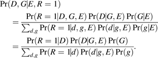 |
(A3) |
Here, R = 1 is an indicator denoting ascertainment into the case-control sample, and P(D|G,E) follows the logistic model A1. For rare diseases, Chatterjee and Carroll note that estimating the nuisance parameters, μ1 ∞ Pr(R|D = 1) and μ0 ∞ Pr(R|D = 0), can be problematic. However, external information about the marginal probability of the disease in the population can be incorporated to improve efficiency of parameter estimation. We assume that the population genotype distribution P(G) follows Hardy-Weinberg proportions and estimate the minor allele frequency using cases and controls combined (effectively weighted by sampling fractions for cases and controls). Unlike the case-only approach, the semiparametric maximum-likelihood estimation uses data from both cases and controls and, hence, can estimate all parameters of interest; moreover, because of the additional Hardy-Weinberg equilibrium assumption, the semiparametric maximum-likelihood estimation estimates of βGE differ slightly from the case-only estimates.
Hedge methods.
Empirical Bayes-type shrinkage estimator (“EB Shrinkage”).
Mukherjee and Chatterjee (8) use an empirical Bayes (EB)-type shrinkage estimation framework for testing G-E interactions. Their interaction estimator () is a weighted average of the standard case-control () and case-only () estimators of the interaction defined in A1 and A2 above. Weights are based on the variance of the case-control estimate and , where is the regression coefficient from the test of G-E independence among controls (i.e., is the log odds ratio from a logistic regression of E on G). These weights are used in an empirical-Bayes fashion to obtain an estimator that “shrinks” toward either the estimated interaction odds ratio under a general model for G-E dependence or toward the estimate obtained under the assumption of G-E independence, depending on the evidence for or against G-E independence:
| (A4) |
The estimated variance of this estimate is
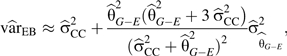 |
(A5) |
which is used to construct the test statistic T = βEB/√varEB, which is asymptotically distributed as a standard normal random variable. The expressions for and were derived for the special case of a binary genotype and binary exposure, with no covariate adjustment. Our application involves an ordinal coding for the genotype; we adopted expressions A4 and A5 for computational simplicity, relying on the fact that, for most SNPs, the ordinal and dominant codings yield similar results. In principle, however, one can calculate the appropriate empirical-Bayes estimates for general genotype and exposure codings and for general covariate adjustment, using the semiparametric maximum-likelihood estimation framework, as described in Mukherjee and Chatterjee (8).
Two-stage.
Murcray et al. (7) propose a simple 2-stage procedure for testing of G-E interactions. In stage 1, they perform a likelihood ratio test of association between G and E based on a logistic model. This is similar to the case-only analysis (A2), but in this context, the test is applied to the combined sample of cases and controls. If the P value for the test is above some prespecified α1, then there is no interaction between G and E. Otherwise, in stage 2, the SNPs that pass stage 1 are assessed in the standard case-control test (A1) for G-E interaction. By testing markers in the second stage using standard logistic regression, this procedure maintains a nominal type I error rate even in the presence of G-E dependence. Significance at this stage is defined as having a P value less than α/m, where α is the desired overall type I error rate and m is the number of tests that pass stage 1. The greater the portion of SNPs associated with E, or increasing α1, leads to an increase in m and reduced power of the method. Applying stage 1 to the entire sample, rather than to cases only, eliminates the correlation between tests in stages 1 and 2 and preserves the overall type I error rate (7).
Two df tests
Joint 2 df.
The joint test combines information about genetic main effects and G-E interaction, with no assumption of G-E independence or Hardy-Weinberg equilibrium. The test uses the same likelihood as the standard test for G-E interaction (A1) but constrains both βg = 0 and βge = 0 under the null and, thus, has 2 df (9).
Joint semiparametric maximum-likelihood estimation (semi-MLE 2 df).
The semiparametric maximum-likelihood estimation 2 df test applies the same assumptions and estimation techniques defined in A3 but, like the joint test described previously, constrains both the genetic main effect and G-E interaction parameters resulting in a 2 df test (4).
Marginal genetic effect
For comparison purposes, we also present results from the case-control test for marginal genetic effects, by testing βg = 0 in the models:
| (A6) |
| (A7) |
The marginal-effect parameter βg in models A6 and A7 represents the effect of G averaged over the distribution of sampled exposures and, thus, is distinct from the main-effect parameter βg in model A1.
Theoretical power calculations
Power calculations for the case-only tests of gene-environment interaction allowing for the presence of gene-environment correlation in the study base were performed by using the method described by Lindström et al. (34) and implemented in the SAS macro GEmis2, available at http://www.hsph.harvard.edu/faculty/peter-kraft/software/. This method is an implementation of the “exemplary data” approach (40) that is also used by Quanto software for power and sample size calculations (http://hydra.usc.edu/GxE/). Specifically, GEmis2 calculates the noncentrality parameter for the test statistic using a logistic regression of binary exposure on genotype for all possible exposure/genotype combinations, weighted by the probability of each combination under a given set of parameters (interaction odds ratio, strength of the G-E correlation in the study base, prevalence of exposure, and so on). The noncentrality parameter can then be used to calculate type I error (when the interaction odds ratio is 1, but the G-E correlation is non-zero) or power and sample size.
For each of the panels in Web Figure 8, we calculated the type I error for a single marker assuming the given genetic odds ratio for exposure (which measures the strength of the gene-environment correlation in the study base). The expected number of false positives was then calculated as N × α1 + (500,000 − N) × α0, where N is the number of markers associated with exposure, α1 is the type I error rate for a marker that is associated with exposure, and α0 is the nominal type I error rate (5 × 10⁻⁸). The probability of at least 1 false positive was calculated as 1 − (1 − α1)N(1 − α0)500,000 − N.
References
- 1.Dempfle A, Scherag A, Hein R, et al. Gene-environment interactions for complex traits: definitions, methodological requirements and challenges. Eur J Hum Genet. 2008;16(10):1164–1172. doi: 10.1038/ejhg.2008.106. [DOI] [PubMed] [Google Scholar]
- 2.Hwang SJ, Beaty TH, Liang KY, et al. Minimum sample size estimation to detect gene-environment interaction in case-control designs. Am J Epidemiol. 1994;140(11):1029–1037. doi: 10.1093/oxfordjournals.aje.a117193. [DOI] [PubMed] [Google Scholar]
- 3.Piegorsch WW, Weinberg CR, Taylor JA. Non-hierarchical logistic models and case-only designs for assessing susceptibility in population-based case-control studies. Stat Med. 1994;13(2):153–162. doi: 10.1002/sim.4780130206. [DOI] [PubMed] [Google Scholar]
- 4.Chatterjee N, Carroll RJ. Semiparametric maximum likelihood estimation exploiting gene-environment independence in case-control studies. Biometrika. 2005;92(2):399–418. [Google Scholar]
- 5.Satten GA, Epstein MP. Comparison of prospective and retrospective methods for haplotype inference in case-control studies. Genet Epidemiol. 2004;27(3):192–201. doi: 10.1002/gepi.20020. [DOI] [PubMed] [Google Scholar]
- 6.Albert PS, Ratnasinghe D, Tangrea J, et al. Limitations of the case-only design for identifying gene-environment interactions. Am J Epidemiol. 2001;154(8):687–693. doi: 10.1093/aje/154.8.687. [DOI] [PubMed] [Google Scholar]
- 7.Murcray CE, Lewinger JP, Gauderman WJ. Gene-environment interaction in genome-wide association studies. Am J Epidemiol. 2009;169(2):219–226. doi: 10.1093/aje/kwn353. [DOI] [PMC free article] [PubMed] [Google Scholar]
- 8.Mukherjee B, Chatterjee N. Exploiting gene-environment independence for analysis of case-control studies: an empirical Bayes-type shrinkage estimator to trade-off between bias and efficiency. Biometrics. 2008;64(3):685–694. doi: 10.1111/j.1541-0420.2007.00953.x. [DOI] [PubMed] [Google Scholar]
- 9.Kraft P, Yen YC, Stram DO, et al. Exploiting gene-environment interaction to detect genetic associations. Hum Hered. 2007;63(2):111–119. doi: 10.1159/000099183. [DOI] [PubMed] [Google Scholar]
- 10.Ritchie MD, Hahn LW, Roodi N, et al. Multifactor-dimensionality reduction reveals high-order interactions among estrogen-metabolism genes in sporadic breast cancer. Am J Hum Genet. 2001;69(1):138–147. doi: 10.1086/321276. [DOI] [PMC free article] [PubMed] [Google Scholar]
- 11.Lunetta KL, Hayward LB, Segal J, et al. Screening large-scale association study data: exploiting interactions using random forests [electronic article] BMC Genet. 2004;5(1):32. doi: 10.1186/1471-2156-5-32. (doi:10.1186/1471-2156-5-32) [DOI] [PMC free article] [PubMed] [Google Scholar]
- 12.Strobl C, Boulesteix AL, Kneib T, et al. Conditional variable importance for random forests [electronic article] BMC Bioinformatics. 2008;9:307. doi: 10.1186/1471-2105-9-307. (doi:10.1186/1471-2105-9-307) [DOI] [PMC free article] [PubMed] [Google Scholar]
- 13.Cupples LA, Bailey J, Cartier KC, et al. Data mining. Genet Epidemiol. 2005;29(suppl 1):S103–S109. doi: 10.1002/gepi.20117. [DOI] [PubMed] [Google Scholar]
- 14.Cordell HJ. Detecting gene-gene interactions that underlie human diseases. Nat Rev Genet. 2009;10(6):392–404. doi: 10.1038/nrg2579. [DOI] [PMC free article] [PubMed] [Google Scholar]
- 15.Mukherjee B, Ahn J, Gruber SB, et al. Tests for gene-environment interaction from case-control data: a novel study of type I error, power and designs. Genet Epidemiol. 2008;32(7):615–626. doi: 10.1002/gepi.20337. [DOI] [PubMed] [Google Scholar]
- 16.Hindorff LA, Junkins HA, Hall PN, et al. A Catalog of Published Genome-Wide Association Studies. Vol 2010. Bethesda, MD: National Human Genome Research Institute; 2010. [Google Scholar]
- 17.Qi L, Hu FB, Hu G. Genes, environment, and interactions in prevention of type 2 diabetes: a focus on physical activity and lifestyle changes. Curr Mol Med. 2008;8(6):519–532. doi: 10.2174/156652408785747915. [DOI] [PubMed] [Google Scholar]
- 18.Thompson WD. Effect modification and the limits of biological inference from epidemiologic data. J Clin Epidemiol. 1991;44(3):221–232. doi: 10.1016/0895-4356(91)90033-6. [DOI] [PubMed] [Google Scholar]
- 19.Siemiatycki J, Thomas DC. Biological models and statistical interactions: an example from multistage carcinogenesis. Int J Epidemiol. 1981;10(4):383–387. doi: 10.1093/ije/10.4.383. [DOI] [PubMed] [Google Scholar]
- 20.Greenland S. Basic problems in interaction assessment. Environ Health Perspect. 1993;101(suppl 4):59–66. doi: 10.1289/ehp.93101s459. [DOI] [PMC free article] [PubMed] [Google Scholar]
- 21.Greenland S. Interactions in epidemiology: relevance, identification, and estimation. Epidemiology. 2009;20(1):14–17. doi: 10.1097/EDE.0b013e318193e7b5. [DOI] [PubMed] [Google Scholar]
- 22.Thorleifsson G, Walters GB, Gudbjartsson DF, et al. Genome-wide association yields new sequence variants at seven loci that associate with measures of obesity. Nat Genet. 2009;41(1):18–24. doi: 10.1038/ng.274. [DOI] [PubMed] [Google Scholar]
- 23.Willer CJ, Speliotes EK, Loos RJ, et al. Six new loci associated with body mass index highlight a neuronal influence on body weight regulation. Nat Genet. 2009;41(1):25–34. doi: 10.1038/ng.287. [DOI] [PMC free article] [PubMed] [Google Scholar]
- 24.Li D, Conti DV. Detecting gene-environment interactions using a combined case-only and case-control approach. Am J Epidemiol. 2009;169(4):497–504. doi: 10.1093/aje/kwn339. [DOI] [PMC free article] [PubMed] [Google Scholar]
- 25.Aschard H, Hancock DB, London SJ, et al. Genome-wide meta-analysis of joint tests for genetic and gene-environment interaction effects. Hum Hered. 2010;70(4):292–300. doi: 10.1159/000323318. [DOI] [PMC free article] [PubMed] [Google Scholar]
- 26.Greenland S, Rothman K. Concepts of interaction. In: Rothman K, Greenland S, editors. Modern Epidemiology. Philadelphia, PA: Lippincott Williams & Wilkins; 1998. [Google Scholar]
- 27.Richardson DB, Kaufman JS. Estimation of the relative excess risk due to interaction and associated confidence bounds. Am J Epidemiol. 2009;169(6):756–760. doi: 10.1093/aje/kwn411. [DOI] [PMC free article] [PubMed] [Google Scholar]
- 28.Skrondal A. Interaction as departure from additivity in case-control studies: a cautionary note. Am J Epidemiol. 2003;158(3):251–258. doi: 10.1093/aje/kwg113. [DOI] [PubMed] [Google Scholar]
- 29.Qi L, Cornelis MC, Kraft P, et al. Genetic variants at 2q24 are associated with susceptibility to type 2 diabetes. Meta-Analysis of Glucose and Insulin-related traits Consortium (MAGIC). Diabetes Genetics Replication and Meta-analysis (DIAGRAM) Hum Mol Genet. 2010;19(13):2706–2715. doi: 10.1093/hmg/ddq156. [DOI] [PMC free article] [PubMed] [Google Scholar]
- 30.Laurie CC, Doheny KF, Mirel DB, et al. Quality control and quality assurance in genotypic data for genome-wide association studies. Genet Epidemiol. 2010;34(6):591–602. doi: 10.1002/gepi.20516. [DOI] [PMC free article] [PubMed] [Google Scholar]
- 31.Willett W, Stampfer MJ, Bain C, et al. Cigarette smoking, relative weight, and menopause. Am J Epidemiol. 1983;117(6):651–658. doi: 10.1093/oxfordjournals.aje.a113598. [DOI] [PubMed] [Google Scholar]
- 32.Murcray CE, Lewinger JP, Conti DV, et al. Sample size requirements to detect gene-environment interactions in genome-wide association studies. Genet Epidemiol. 2011;35(3):201–210. doi: 10.1002/gepi.20569. [DOI] [PMC free article] [PubMed] [Google Scholar]
- 33.Purcell S, Neale B, Todd-Brown K, et al. PLINK: a tool set for whole-genome association and population-based linkage analyses. Am J Hum Genet. 2007;81(3):559–575. doi: 10.1086/519795. [DOI] [PMC free article] [PubMed] [Google Scholar]
- 34.Lindström S, Yen YC, Spiegelman D, et al. The impact of gene-environment dependence and misclassification in genetic association studies incorporating gene-environment interactions. Hum Hered. 2009;68(3):171–181. doi: 10.1159/000224637. [DOI] [PMC free article] [PubMed] [Google Scholar]
- 35.Tchetgen Tchetgen EJ, Kraft P. On the robustness of tests of genetic associations incorporating gene-environment interaction when the environmental exposure is misspecified. Epidemiology. 2011;22(2):257–261. doi: 10.1097/EDE.0b013e31820877c5. [DOI] [PMC free article] [PubMed] [Google Scholar]
- 36.Grant SF, Thorleifsson G, Reynisdottir I, et al. Variant of transcription factor 7-like 2 (TCF7L2) gene confers risk of type 2 diabetes. Nat Genet. 2006;38(3):320–323. doi: 10.1038/ng1732. [DOI] [PubMed] [Google Scholar]
- 37.Clayton D, McKeigue PM. Epidemiological methods for studying genes and environmental factors in complex diseases. Lancet. 2001;358(9290):1356–1360. doi: 10.1016/S0140-6736(01)06418-2. [DOI] [PubMed] [Google Scholar]
- 38.Bhattacharjee S, Wang Z, Ciampa J, et al. Using principal components of genetic variation for robust and powerful detection of gene-gene interactions in case-control and case-only studies. Am J Hum Genet. 2010;86(3):331–342. doi: 10.1016/j.ajhg.2010.01.026. [DOI] [PMC free article] [PubMed] [Google Scholar]
- 39.Ottman R. Gene-environment interaction: definitions and study designs. Prev Med. 1996;25(6):764–770. doi: 10.1006/pmed.1996.0117. [DOI] [PMC free article] [PubMed] [Google Scholar]
- 40.Longmate JA. Complexity and power in case-control association studies. Am J Hum Genet. 2001;68(5):1229–1237. doi: 10.1086/320106. [DOI] [PMC free article] [PubMed] [Google Scholar]
Associated Data
This section collects any data citations, data availability statements, or supplementary materials included in this article.