Measuring Flux Distributions for Diffusion in the Small-Numbers Limit

Abstract

For the classical diffusion of independent particles, Fick's law gives a well-known relationship between the average flux and the average concentration gradient. What has not yet been explored experimentally, however, is the dynamical distribution of diffusion rates in the limit of small particle numbers. Here, we measure the distribution of diffusional fluxes using a microfluidics device filled with a colloidal suspension of a small number of microspheres. Our experiments show that (1) the flux distribution is accurately described by a Gaussian function; (2) Fick's law, that the average flux is proportional to the particle gradient, holds even for particle gradients down to a single particle difference; (3) the variance in the flux is proportional to the sum of the particle numbers; and (4) there are backward flows, where particles flow up a concentration gradient, rather than down it. In addition, in recent years, two key theorems about nonequilibrium systems have been introduced: Evans' fluctuation theorem for the distribution of entropies and Jarzynski's work theorem. Here, we introduce a new fluctuation theorem, for the fluxes, and we find that it is confirmed quantitatively by our experiments.

I. Introduction

Fick's law, which describes the diffusion of atoms, molecules, and particles, is important in many areas of science and is the basis for engineering models of material transport. According to Fick's first law, the average particle flux is proportional to the average concentration gradient:¹

$$\langle J\rangle =-D\frac{\partial \langle c\rangle }{\partial x}$$ (1)

where 〈J〉 is the observed macroscopic flux and 〈c〉 is the concentration of particles. We use brackets here, 〈…〉, to make it explicit that this phenomenological expression deals with averages over macroscopically large numbers of particles and to indicate that only in macroscopic systems can the particle concentration and flux be meaningfully represented as smooth functions of space and time. Fick's first law is the basis for Fick's second law, also known as the diffusion equation:

$$\frac{\partial \langle c\rangle }{\partial t}=D\frac{{\partial }^2\langle c\rangle }{\partial x^2}$$ (2)

These equations have been verified extensively in bulk gases and solutions with macroscopically large numbers of particles.²

Our particular interest here is in the “small-numbers” limit of diffusion, where there are only a few particles in the system and where the fluctuations can be large. Small particle numbers and their fluctuations are important (a) in nanotechnology, (b) inside biological cells, where the typical copy number of any given type of protein is often less than a few thousand,³ and (c) in single-molecule studies of ion channels, molecular motors, and laser trap experiments,^4–6 for example. Fick's law describes averages over a macroscopic number of particles; it does not describe small-number fluctuational quantities, such as 〈J²〉 − 〈J〉², or other aspects of the flux distribution function. One of our motivations for undertaking this work is a growing interest in nonequilibrium dynamics in small-numbers systems. We reasoned that a first step in examining the distribution of microtrajectories in nonequilibrium systems would be to revisit classical systems such as simple diffusion where the average properties are well-established. Only recently has it become possible to perform experiments on small-numbers diffusion and to measure full dynamical distribution functions, based on advances in nanotechnology, video microscopy, and microfluidics.

Does Fick's law hold in the limit of small numbers of particles? And, are there violations? That is, if Fick's law predicts flow to the right, due to a concentration gradient sloping downward toward the right, does it ever happen that particles flow instead to the left? Such situations have been called “second-law violations”,^7,8 or in classical thermal problems, they are expressed in terms of “Maxwell's demon”.⁹ Such fluctuations are, of course, not real violations of the second law, because the second law is only a statement about averages, not fluctuations.¹⁰ In this article, we refer instead to such trajectories that go “against the grain” as bad actors.

What dynamical distribution of rates would be expected from theory? We describe below the results from a maximum-entropy-like approach,¹¹ called maximum caliber, based on the work of E. T. Jaynes.¹² Other approaches based on random-flight modeling should lead to the same result. In short, if particles are independent, diffusing in one dimension, and if their jump rates are stationary in time, the distribution of particle fluxes, P(J), at time t along an x-axis from one bin at x having N₁ particles to an adjacent bin at x + Δx having N₂ particles, should follow the binomial distribution, or approximately a Gaussian function:¹¹

$$\begin{array}{cc}\hfill P\left(J\right)& =\frac{1}{\sqrt{2\pi \langle {\left(\Delta J\right)}^2\rangle }}\text{exp}\left(-\frac{{(J-\langle J\rangle )}^2}{2\langle {\left(\Delta J\right)}^2\rangle }\right)\hfill \\ \hfill & =\frac{1}{\sqrt{2\pi \left(\mathit{pqN}\right)}}\text{exp}\left(-\frac{{(J-p\Delta N)}^2}{2\mathit{pqN}}\right)\hfill \end{array}$$ (3)

where ΔN = N₁ − N₂, N = N₁ + N₂, 〈ΔJ²〉 is the variance in the flux, J, and q = 1 − p, with p being the probability that a particle jumps in the time interval, Δt.

Various moments of the distribution function are readily obtained from this approach. First, the model predicts that the average net number of particles, J, that jump per unit time at time t is¹¹

$$\langle J\rangle =\langle j_1-j_2\rangle =-\frac{p}{\Delta t}\Delta N$$ (4)

where j₁ is the flux from bin 1 at x to bin 2 at x + Δx and j₂ is from bin 2 to 1. This proportionality of the average flux, 〈J〉, to ΔN simply predicts Fick's law, where the diffusion coefficient, D, is related to p by D = pΔx²/Δt, and where Δx is the bin size and Δt is the unit time step.

For the flux fluctuations, that is, the second moment, the model predicts

$$\langle \Delta J^2\rangle =\langle {(J-\langle J\rangle )}^2\rangle =\frac{p(1-p)}{\Delta t^2}N$$ (5)

where N = N₁ + N₂ is the total number of particles associated with the two bins of interest. Hence, the key prediction here is that the flux fluctuations are proportional to the total particle number, N.

We are also interested in the number of bad actors, that is, the number of trajectories that would lead to particle flows up a concentration gradient, rather than down it. This quantity can be derived from the flux distribution¹¹ as

$${\Phi }_{\text{badactors}}=\frac{1}{2}\left(1-\text{erf}\left(\frac{\langle J\rangle }{\sqrt{2\langle {\left(\Delta J\right)}^2\rangle }}\right)\right)\approx \frac{1}{2}-\frac{1}{\sqrt{2\pi }}\frac{\langle J\rangle }{\sqrt{\langle {\left(\Delta J\right)}^2\rangle }}\dots +\mathcal{Q}\left\{{\left(\frac{\langle J\rangle }{\sqrt{\langle {\left(\Delta J\right)}^2\rangle }}\right)}^3\right\}$$ (6)

where the approximation holds for small values of $\langle J\rangle ∕\sqrt{\langle {\left(\Delta J\right)}^2\rangle }$. In the expression above, the next higher term (the cubic term) is an order of magnitude smaller than the linear term for the values of $\langle J\rangle ∕\sqrt{\langle {\left(\Delta J\right)}^2\rangle }$ used in our experiments (see Figure 3).

Figure 3.

Fraction of trajectories that are bad actors vs the deviation from equilibrium as characterized by the normalized mean flux, $\langle J\rangle ∕\sqrt{2\langle {\left(\Delta J\right)}^2\rangle }$. Experimental data are shown in squares, while the solid line represents the fit to the data. The coefficient of determination, R², for the fit is also reported. The slope and intercept agree well with the model.

A. A “Flux Fluctuation Theorem”

Recent work has led to fluctuation theorems that have provided important insights into nonequilibrium systems. Fluctuation theorems describe the extent to which a system deviates from its dominant flow behavior.^8,13–16 In the diffusive dynamics case of interest here, if the number of particles, N₁, in bin 1 is greater than the number of particles, N₂, in bin 2, then particles, on average, will flow from 1 to 2. Fluctuation theorems describe the amount of reverse flow, that is, up the concentration gradient in this case. One such theorem^8,13 expresses such flows in terms of the probabilities of entropy changes in the forward and backward directions, P(ΔS)/P(−ΔS). And, the work theorems of Jarzynski and Crooks express the probabilities, P[w/(kT)]/P[−w/(kT)], of the work, w, in the two directions.¹⁷

Ours is a fluctuation theorem about the flux, J. We compute P(J)/P(−J), the ratio of probabilities of fluxes in the forward and backward directions, using eq 3:¹¹

$$\text{ln}\frac{P\left(J\right)}{P(-J)}=\frac{2\langle J\rangle }{\langle {\left(\Delta J\right)}^2\rangle }J$$ (7)

Thus, the quantity ln[P(J)/P(−J)] is predicted to be proportional to the normalized flux, 〈J〉/〈(ΔJ)²〉 × J. In situations having large flux, the back-flow becomes exponentially negligible. We subjected these predictions to experimental tests, described below.

II. The Microfluidics Experiments

To study the dynamical distributions in diffusion, we devised a microfluidics experiment. Using the techniques of soft lithography, chip fabrication,¹⁸ and the Sylgard 184 Silicone elastomer kit (Dow Corning Corporation), we made a microfluidics chamber having approximate dimensions of 400 μm by 100 μm, partitioned into two regions (see Figure 1a). The cross section of this chamber is a segment of a circular disc, with a maximum depth of 10 μm (see Figure 1b). The chamber is filled on one side with a solution containing about 200 colloidal, green fluorescent polystyrene particles 0.29 μm in diameter (Duke Scientific, Cat. No. G300) (see Figure 1a). The beads are at an optimized concentration so that the interactions are negligible¹⁹ while at the same time permitting sufficient statistics over a wider range of ΔN and N.

Figure 1.

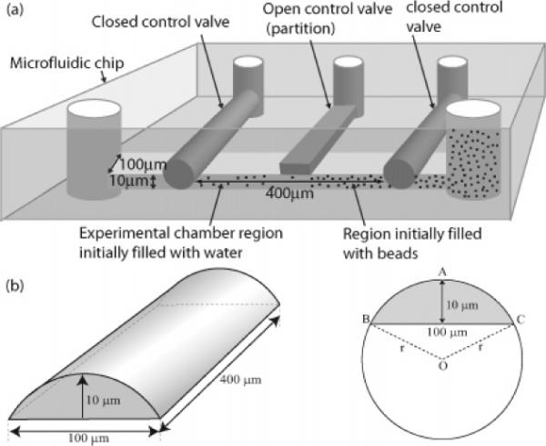
Microfluidics experiment. Colloids corralled on one side of a gate begin to diffuse at time t = 0 by opening the gate. (a) Schematic of the microfluidic chip (see text for details). (b) The geometry of the microfluidic chamber (not drawn to scale).

At time t = 0, we open a microfluidic gate (i.e., a partition), allowing particles to diffuse from one side to the other, taking periodic snapshots under an Olympus IX71 inverted microscope. (We performed the same experiment under equilibrium conditions where the initial concentration was uniform across the whole chamber (results not shown, see ref 20).) We take three snapshots of the beads in the chamber every time interval of Δt = 10 s, for 6 h. Since there is a possibility that some particles temporarily overlap and/or are out of focus in a single snapshot, taking three snapshots of each minimizes that error to 1–2%, which corresponds to 2–4 particles out of the 200. The snapshots are taken using fluorescence microscopy with a SONY DFW-V500 camera. (During the time when no snapshots are taken, a shutter prevents the experimental chamber from being exposed to the incident light, to prevent photobleaching and heating the chamber.) We then determine the particle positions at each snapshot using a computerized centroid tracking algorithm.²⁵

The time-dependent particle density is determined by dividing the chamber into a number of equal-sized bins of value Δx each along the longest dimension of 400 μm and by computing the number of particles in each bin as a function of time. Although the microfluidic chamber is three-dimensional, it can be shown that, in the case of weak particle–particle and particle–wall interactions, the problem can be collapsed to a one-dimension diffusion problem. Therefore, we bin only along the x-axis, the direction of the concentration gradient.

As expected from the equations presented in the previous section, eqs 3–7, the results presented below are independent of the choice of the bin size for bin sizes that are reasonable (i.e., clearly bins with a size compared to the entire chamber are not useful). Indeed, different values for the bin size were used for the data analysis, all producing results that agree with the ones shown in section III. However, the choice of the bin size affects the statistics for each combination of N₁ and N₂ as well as the range of N and ΔN themselves. If the bins are too wide, then there will not be enough statistics and the range of values for N will not include small numbers (since it will be rare to have one or two particles in a single bin). On the other hand, if the bin size is too small, we may not have a sufficient range of values for N and ΔN (since small bins will rarely have more than a few particles). Also, if the bins are too small, a particle may jump across multiple bins within the time interval, Δt. Therefore, the optimal choice of the bin size was made on the basis of the bead's expected mean excursion within the time interval, Δt, which is x$\sqrt{2D\Delta t}$. This is the only relevant microscopic length scale. Here, D is the diffusion coefficient for an individual bead given by the Stokes formula.²⁶

For a bead of 0.29 μm in diameter suspended in water at room temperature, the Stokes formula gives a diffusion coefficient, D, of approximately 1.5 μm²/s. This value, within experimental error, is equal to the one we obtain by fitting our data of the concentration profile at different times to the one-dimensional diffusion equation using D as our fitting parameter (i.e., D = 1.3 ± 0.27 μm²/s). This gives a bin size of Δx ≈ 5 μm. By observing all the consecutive bin pairs for all the frames taken, we were able to obtain, on average, about 5000 points for each combination of N₁ and N₂. Given the bead concentration in the microfluidics channel, N₁ and N₂ ranged from 0 to 6. The choice of bin size determines the value of the jump probability, p, as discussed in ref 21.

We can find the flux at a plane i at a specific time interval from the computed particle distribution statistics as a function of position x and time t mentioned above. Since the microfluidic chamber is isolated, the total number of particles stays the same from one frame to the next. As a result of this conservation in particle number, the flux at plane i + 1, J_i+1, that is, the plane that separates bins i and i + 1, can be easily evaluated by using the continuity equation:

$$N_i(t+\Delta t)=N_i\left(t\right)+(J_i\left(t\right)-J_{i+1}\left(t\right))\Delta t$$ (8)

$$\Rightarrow J_{i+1}\left(t\right)=-\frac{N_i(t+\Delta t)-N_i\left(t\right)}{\Delta t}+J_i\left(t\right)$$ (9)

where N_i is the number of particles in bin i. Since the microfluidic chamber is isolated, from our boundary conditions, the flux J₀ (flux at x = 0) is zero at all times. Combined with eq 9, we obtain J₁(t). Thus, from the analysis of these images, we obtain complete sets of the values of {N_i(t)} and {J_i(t)} in all of the bins and at all times of observation. Then, for each pair of consecutive bins with specific values of N₁ and N₂, we construct the histogram of J values. Upon normalization, the histogram becomes the flux probability distribution, P(J).

III. Results

A. The Flux Distribution is a Gaussian Function

Figure 2 shows our observed particle flux distribution function at the optimized concentration. All of the data fall on a single master curve where 〈J〉 and 〈(ΔJ)²〉 have been calculated separately from each combination of N₁ and N₂. The quadratic form observed on this log plot shows that the distribution function is given accurately by a Gaussian. The theory predicts that (i) the coefficient of the square term should be −1, (ii) the coefficient of the linear term should be zero, and (iii) the constant term should be ln$(\Delta J_{\mathrm{bin}}∕\sqrt{2\pi })\approx -0.9$, where ΔJ_bin is the bin size used to obtain the histogram and is equal to 0.1 s⁻¹, that is, one particle per unit time. Consistent with these predictions, the coefficient observed for the square term is −0.98, that for the linear term is −0.0018, and that for the constant term is −0.94. The coefficient of determination for the quadratic fit is R² = 0.98.

Figure 2.

Flux distribution function. ½ ln(〈(ΔJ)²〉) + ln(P(J)) is plotted against ($(J-\langle J\rangle )∕\sqrt{2\langle {\left(\Delta J\right)}^2\rangle }$, based on the form indicated by eq 3. The circles indicate experimental points, and the line shows a quadratic fit to the data. The coefficient of determination, R², for the fit is also reported. This demonstrates that the distribution function is Gaussian, and we find that the coefficients are well predicted by eq 3.

Next, we analyze the bad actors–the backward flows–in two different ways.

B. The Bad-Actor Trajectory Counts are Well Predicted by the Model

Equation 6 predicts that, for small values of $\langle J\rangle ∕\sqrt{\langle {\left(\Delta J\right)}^2\rangle }$, the fraction of bad actors should be linearly proportional to $\langle J\rangle ∕\sqrt{\langle {\left(\Delta J\right)}^2\rangle }$. In good agreement, Figure 3 confirms this linearity and gives the predicted intercept of 0.5. This means that, as the system approaches equilibrium (i.e., 〈J〉 ≈ 0), about half the trajectories involve flow down the vanishingly small gradient and half the trajectories involve flow up that small gradient. In the linear regime, the best fit line shows the slope to be 0.37, which agrees well with the expected value of $1∕\sqrt{2\pi }\approx 0.4$ from eq 6. The coefficient of determination for the linear fit is R² = 0.99. This figure shows that when the system is more distant from equilibrium (as implied by a larger mean flux), there are fewer bad actors. Expressed differently, far from equilibrium, more trajectories are “potent”; they are able to change the current state of the system.¹¹

C. Testing the Flux Fluctuation Theorem

Figure 4 shows ln(P(J)/P(−J)) versus the flux, normalized by 〈J〉J/〈(ΔJ)²〉, to account for different averages and variances of the flux distribution. This rescaling leads to a linear master curve, as predicted by eq 7. There are four outlying points which clearly deviate from the linear curve. A possible explanation for these outliers comes from the fact that the quantity plotted in the y-axis is a ratio and this results in error magnification. Therefore, one needs very small error in the flux distribution itself in order to minimize the error in P(J) and P(−J) and avoid uncertainties in their ratio, P(J)/P(−J). Possible sources of error for the deviant points can be the nonconservation in the particle number and/or insufficient statistics. Both of these would lead to inaccurate values of P(J) and, thus, to outlying points. However, these outliers do have sufficient statistics, so we believe that they are the result of the nonconservation in the particle number. In other words, the very construction of the variable plotted in the y-axis makes it sensitive to the actual measurement unlike the averages or the histogram shown in other graphs. However, it is still clear from the plot that the experiments show the slope to be 2.0, in perfect agreement with the predicted slope of 2 from eq 7, where R² = 0.77. This and other fluctuation theorems provide a compact way to quantitate the bad-actor microtrajectories.

Figure 4.

Flux fluctuation theorem. The plot shows ln[P(J)/P(−J)] vs 〈J〉J/〈(ΔJ)²〉 for different values of 〈J〉 and 〈(ΔJ)²〉 arising due to different combinations of N₁ and N₂. Experimental data are shown in circles, while the solid line represents the fit to the data. The coefficient of determination, R², for the fit is also reported. The slope and intercept agree with the prediction of eq 7.

D. Fick's Law Holds Even in the Small-Numbers Limit

We compare the average flux between two neighboring bins, 〈J〉, with the difference in particle numbers, ΔN = N₁ − N₂. This data is compiled from all the values of N₁ and N₂ that provide a given ΔN value. Figure 5 shows that 〈J〉 depends linearly on the particle number gradient, ΔN, even down to “gradients” of zero or one particle, indicating that Fick's law holds in the small-numbers limit. The slope of the graph (0.03/s) also gives us a value of the jump rate, p = 0.3, which is in good agreement with the theoretical estimate of 0.33 made in terms of the bin size and the diffusion coefficient.²¹ As expected, the intercept is close to 0 (see eq 4). The linear fit has a coefficient of determination of R² = 0.99.

Figure 5.

Experimental support for Fick's law, even down to few-particle gradients. The average flux, 〈J〉, is shown as a function of ΔN, the gradient in the particle number between two neighboring bins. Experimental data are shown in circles, while the solid line represents the fit to the data. The coefficient of determination, R², for the fit is also reported. The error bars shown are the variances due to the different combinations of N₁ and N₂ resulting in the same ΔN. The slope and intercept are in agreement with the expected theoretical values, based on eq 4.

E. The Second Moment of Particle Flux is Proportional to the Sum of Particle Numbers

Equation 5 predicts that the second moment of the flux should be proportional to the sum of particle numbers in the two bins, N = N₁ + N₂. Figure 6 confirms this dependence of 〈ΔJ²〉 = 〈(J − 〈J〉)²〉 on N. For the optimized particle concentrations, the slope (0.0022/s²) is equal to the expected slope of 0.0022/s² for the value of p = 0.33, with R² = 0.96. At higher particle concentrations (data not shown), however, not surprisingly, systematic errors begin to appear and the slope deviation is quite high compared to the expected value. We performed Brownian dynamics simulations that show the likely cause of these concentration-dependent errors is nonconservation of bin counts, from particles that either overlap or go out of focus in one snapshot and into focus in the next (see previous section).

Figure 6.

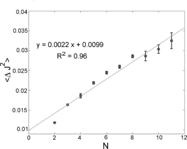
Second cumulant, 〈ΔJ²〉) 〈J²〉 − 〈J〉², vs the total number of particles, N. The second moment of particle flux is proportional to the sum of particle numbers in the two bins. Experimental data are shown in circles, while the solid line represents the fit to the data. The coefficient of determination, R², for the fit is also reported. The error bars show the variances due to the different combinations of N₁ and N₂ that result in the same N value. The slope and intercept are well predicted by eq 5.

IV. Conclusions

Whereas Fick's law of average diffusion is well-established, the distribution function of diffusional rates has not been so widely studied. Recent advances in microfluidics now make it possible to study diffusion in the limit of small particle numbers. We describe here a microfluidics experiment with which we determine the distribution of particle fluxes in few-particle diffusion. We find that the flux is distributed according to a Gaussian distribution function. With only a single parameter p, which is essentially the diffusion constant, elementary theory gives several results that are confirmed by the experiments. First, we find that Fick's law–the proportionality of average flux to the gradient of average concentration–holds even down to concentration gradients as small as a single particle. Experiments also confirm that the variance in the flux is proportional to the total number of particles, 〈J²〉 ∝ N₁ + N₂, with correct slopes within experimental errors. In addition, we introduce a new flux fluctuation theorem, that is found to be consistent with the data in predicting an exponentially diminishing number of variant trajectories, as a function of the deviation from equilibrium. It is an analog of quantities of recent interest in other nonequilibrium experiments.^8,14–16 The model predicts the backward flows, the bad actors, which are relatively infrequent situations in which particles flow up, rather than down, their concentration gradients. These experiments provide extensive data that go beyond more traditional phenomenological average flux quantities and illuminate the nature of dynamical fluctuations in a simple classical system.

References and Notes

- (1).Dill K, Bromberg S. Molecular driving forces: statistical thermodynamics in chemistry and biology. Garland Sciences; New York: 2003. [Google Scholar]
- (2).Baker RW. Controlled release of biologically active agents. Wiley; New York: 1987. [Google Scholar]
- (3).Wu J-Q, Pollard TD. Science. 2005;310:5746. doi: 10.1126/science.1113230. [DOI] [PubMed] [Google Scholar]
- (4).Hille B. Ion channels of excitable membranes. Sinauer Associates; Sunderland, MA: 2001. [Google Scholar]
- (5).Howard J. Mechanics of motor proteins and the cytoskeleton. Sinauer Associates; Sunderland, MA: 2001. [Google Scholar]
- (6).Neuman KC, Block SM. Rev. Sci. Instrum. 2004;75:2787. doi: 10.1063/1.1785844. [DOI] [PMC free article] [PubMed] [Google Scholar]
- (7).Evans DJ, Cohen EGD, Morriss GP. Phys. ReV. Lett. 1993;71(15):2401. doi: 10.1103/PhysRevLett.71.2401. [DOI] [PubMed] [Google Scholar]
- (8).Evans DJ, Searles DJ. Adv. Phys. 2002;51:1529. [Google Scholar]
- (9).Feynman R. Feynman lectures on computation. Perseus; Cambridge, MA: 1996. [Google Scholar]
- (10).Callen HB. Thermodynamics and an introduction to thermostatics. Wiley; New York: 1985. [Google Scholar]
- (11).Ghosh K, Dill K, Inamdar M, Seitaridou E, Phillips R. Am. J. Phys. 2006;74:123. doi: 10.1119/1.2142789. [DOI] [PMC free article] [PubMed] [Google Scholar]
- (12).Jaynes ET. E. T. Jaynes: Papers on probability, statistics and statistical physics. Kluwer; Boston, MA: 1980. [Google Scholar]
- (13).Crooks GE. Phys. Rev. E. 1999;60:2721. doi: 10.1103/physreve.60.2721. [DOI] [PubMed] [Google Scholar]
- (14).Blickle V, Speck T, Helden L, Seifert U, Bechinger C. Phys. Rev. Lett. 2006;96:070603. doi: 10.1103/PhysRevLett.96.070603. [DOI] [PubMed] [Google Scholar]
- (15).Collin D, Ritort F, Jarzynski C, Smith S, Tinoco I, Bustamante C. Nature. 2005;437:231. doi: 10.1038/nature04061. [DOI] [PMC free article] [PubMed] [Google Scholar]
- (16).Feitosa K, Menon N. Phys. Rev. Lett. 2004;94:164301. doi: 10.1103/PhysRevLett.92.164301. [DOI] [PubMed] [Google Scholar]
- (17).Crooks G. Ph.D. Thesis. 1999. [Google Scholar]
- (18).Unger MA, Chou HP, Thorsen T, Scherer A, Quake SR. Science. 2000;288:113. doi: 10.1126/science.288.5463.113. [DOI] [PubMed] [Google Scholar]
- (19).The bead concentration is such that the mean particle spacing is about 8 μm. For such large particle separations, electrostatic22 and hydrodynamic interactions23,24 are negligible. Although the polystyrene particles have a small negative surface charge, it is readily shown using the Poisson–Boltzmann equation that there is little interaction at these separations, and we confirmed that result by an experiment showing an independence on salt concentrations (data not shown). Also, the data of Meiners and Quake23 and Dufresne et al.,24 applied to our system, show that hydrodynamic interactions should be small.
- (20).The results obtained under the equilibrium setting were similar to the ones presented in this paper. However, the equilibrium measurements were not presented, since the local concentration gradient was obviously rather small, thus limiting the range of ΔN values.
- (21).The jump probability, p, in the time interval, Δt, from bin i – 1 to bin i (of size Δx) can be estimated from the diffusion of a particle with diffusion coefficient D. However, there is also a possibility of a jump occurring from any of the other bins to bin i. After summing all of the jump probabilities from all of the neighboring bins, the effective probability, p, is found to be p ≃ 0.33, for the given values of Δx, Δt, and D. (22) Crocker, J. C.; Grier, D. G. Phys. Rev. Lett. 1994, 73, 352.
- 22.Crocker JC, Grier DG. Phys. ReV. Lett. 1994;73:352. doi: 10.1103/PhysRevLett.73.352. [DOI] [PubMed] [Google Scholar]
- (23).Meiners J-C, Quake SR. Phys. Rev. Lett. 1999;82:2211. [Google Scholar]
- (24).Dufresne ER, Squires TM, Brenner MP, Grier DG. Phys. Rev. Lett. 2000;85:3317. doi: 10.1103/PhysRevLett.85.3317. [DOI] [PubMed] [Google Scholar]
- (25).Crocker JC, Grier DG. J. Colloid Interface Sci. 1996;179:298. [Google Scholar]
- (26).Reif F. Fundamentals of statistical and thermal physics. McGraw-Hill; New York: 1965. [Google Scholar]