Circadian desynchronization

Abstract

The suprachiasmatic nucleus (SCN) coordinates via multiple outputs physiological and behavioural circadian rhythms. The SCN is composed of a heterogeneous network of coupled oscillators that entrain to the daily light–dark cycles. Outside the physiological entrainment range, rich locomotor patterns of desynchronized rhythms are observed. Previous studies interpreted these results as the output of different SCN neural subpopulations. We find, however, that even a single periodically driven oscillator can induce such complex desynchronized locomotor patterns. Using signal analysis, we show how the observed patterns can be consistently clustered into two generic oscillatory interaction groups: modulation and superposition. In seven of 17 rats undergoing forced desynchronization, we find a theoretically predicted third spectral component. Combining signal analysis with the theory of coupled oscillators, we provide a framework for the study of circadian desynchronization.

1. Introduction

The mammalian suprachiasmatic nucleus (SCN) contains a master circadian clock that governs the circadian rhythms of physiology and behaviour. Daily light–dark (LD) cycles detected by the eyes entrain about 20 000 neurons in the SCN via signals travelling along the retinohypothalamic tract. The SCN is constituted by a network of single-cell neuronal oscillators that together act as a pacemaker, which regulates circadian rhythms through direct and indirect output pathways to other regions of the brain. It is an open question how individual SCN cells create an integrated pacemaker, which produces a robust and coherent rhythm. Several studies suggest heterogeneity at different levels within the SCN network: studies on SCN slices and dispersed SCN cells revealed that SCN cells have a broad distribution of periods, amplitudes and amplitude-relaxation rates [1,2]. Such diverse SCN neuronal population synchronize via neuropeptide diffusion, synaptic signalling, nitric oxide [3] and gap junctions [4–6].

Experiments elucidating SCN heterogeneity are often invasive and thus implicitly modify the SCN tissue in an unknown manner. Interestingly, a protocol to non-invasively dissociate this circadian oscillatory network in vivo was proposed. Rats exposed to exotic short LD cycles, presumably close to the limits of circadian entrainment (see below), express two stable circadian motor activity rhythms (a fast and a slow rhythm [7–9]). These two stable circadian components depend on the period of the external cycle, i.e. the strength and period of both components are regulated by the external LD cycle [8,10]. Further studies of SCN gene expression under such conditions suggested that these two-motor-activity rhythms reflect the separate activities of two populations of oscillators in anatomically identifiable subregions of the SCN, i.e. ventrolateral and dorsomedial SCN subdivisions [9,11]. The presence of two oscillators in the SCN—one in the vasoactive intestinal polypeptide-containing ventral SCN and one in the vasopressin-containing dorsal SCN—was already proposed by Shinohara et al. [12]. Compartmentalization within the SCN has been observed under different photoperiods and in jet-lag experiments from gene expression level to electrical activity (for a review see [6]). This, so-called ‘forced desynchronization’, protocol was proposed to be the first stable separation of two regional SCN oscillators in vivo [13]. Moreover, a series of experiments exploit this regional SCN separation to investigate the link between known SCN outputs and the ventrolateral or dorsomedial SCN regions [14–17].

Here, we present a detailed study on the ‘forced desynchronization’ experiments from a theoretical perspective. We show how two stable circadian motor activity rhythms can be generated from only one driven oscillator. With oscillatory interactions between the external zeitgeber and the internal circadian clock, we are able to explain all the observed patterns. Furthermore, we predict a third slower circadian component in the activity pattern. Re-analysis of the previously published data confirms this additional component in seven of 17 rats undergoing forced desynchronization. These results can be explained in terms of classical signal analysis: a modulated signal results in spectra containing the original carrier frequency and two mirror-symmetric side-band frequencies. We show that such side-bands can be explained using bifurcation theory of coupled oscillators. Our analysis elucidates a novel mechanism in circadian biology: a slow periodic modulation of the circadian output near the borderline of entrainment regions.

2. Basics of entrainment

To provide a theoretical background, we first summarize established concepts of entrainment and describe the dynamical features observed in the forced desynchronization experiments. In figure 1, we present the generic entrainment results expected from a driven oscillator with an endogenous period of 24 h. Figure 1a schematically describes the concept of oscillator entrainment to external signals (zeitgebers such as light). Zeitgeber cycles interact with the endogenous oscillator in such a way that the frequencies are locked in a 1 : 1 entrainment ratio leading to a stable phase relation between the external signal and the entrained oscillator. Critically, upon release into constant conditions, entrained oscillations persist with a phase predicted from the previous entrained cycles. Note that we do not yet assume anything about the physical nature of the oscillator: it could be a single-cell biochemical oscillator or a synchronized population of cells, such as the SCN. Figure 1b illustrates that the range of entrainment depends on zeitgeber strength. Entrainment is most easily achieved if the endogenous and zeitgeber periods are similar. For example, the circadian behaviour in laboratory rodents can be entrained to zeitgeber cycles with deviations of about 2 h from the endogenous period of ca 24 h. The entrainment range can be enlarged if the zeitgeber strength is increased. Thus, the entrainment region typically shows a tongue-shaped form [18]. For a constant zeitgeber strength, the entrainment region is confined between its lower (T_low) and upper (T_high) limit of entrainment, known as the entrainment range (figure 1b). In circadian biology, the oscillator dynamics is usually represented as a double-plotted actogram, i.e. the activities on two subsequent days are plotted horizontally in each line. While the oscillator state variable values are above a given threshold (figure 1a), the activity is represented as a black horizontal line. In such 24 h double-plot actograms, 24 h rhythms appear as vertical stripes resulting from a superposition of several black horizontal lines (see actograms in figure 1a,d). Shorter (figure 1c) and longer periods (figure 1e) have positive and negative slope stripes, respectively. Within the entrainment region, the oscillator period is locked to the zeitgeber period and thus the spectrum has only one circadian component (figure 1g–i). Consequently, a plot of the main spectral component for different zeitgeber periods within the entrainment region leads to a straight line with slope one (figure 1f). The normalized spectral power of this component exhibits a resonance-like behaviour (figure 1j).

Figure 1.

Basic concepts of entrainment (a) Schematic of a circadian rhythm entrained by 24 h LD cycles. The square-wave light cycles represent the zeitgeber cycle used in the experiments of this study also known as T-cycle. Note that upon complete entrainment, the phase angle relation between rhythmic variable and zeitgeber cycle is constant. (b) Schematic of the entrainment region where the oscillator period is locked to the external period in a 1∶1 relation. The entrainment region is dependent on zeitgeber period (T) and zeitgeber strength and is also known as 1∶1 Arnold tongue. For a constant zeitgeber strength, the entrainment region is confined between its lower (T_low) and upper (T_high) limit of entrainment. Outside the entrainment region, the oscillators show no stable phase relation. Within the entrainment region, the oscillator can be locked to shorter (22 h) and longer (26 h) than 24 h period. The oscillator state variable is typically plotted as a 24 h double-plotted actogram (c–e), i.e. with activity on day n followed by day n + 1 horizontally, succeeded by days n + 1 and n + 2 on the next line, etc. The actogram of an oscillator entrained to 22, 24 and 26 h typically shows positive slope, vertical and negative slope stripes, respectively. Within the entrainment region, the oscillator is locked to the external rhythm and thus the spectra of the oscillator state variable shows only one main component with the period of the zeitgeber (g–i). Thus, the spectral component for different zeitgeber periods leads to a line of slope one (f) and the normalized power of this unique component leads to a resonance-like curve (j). (c–j) was generated with the oscillator model discussed below. Further details are given in §9.

3. Forced desynchronization of rat-activity rhythms

Having established the basic concepts of entrainment, we now revise the main experimental results obtained under the forced desynchronization protocol. In a first series of experiments published in Campuzano et al. [8], six groups of eight rats each were housed individually in 25 × 25 × 12 cm transparent cages and exposed to a symmetric LD cycle with periods of 21, 21.5, 22, 22.5, 23 and 23.5 h. In all cases white light of 300 lux and dim-red light of less than 0.5 lux alternate. Animals were kept under these LD conditions for 60 days and their motor activities were recorded with infrared beams. In more recent experiments published in de la Iglesia et al. [9], 21 two-month-old male Wistar rats were exposed to a 22 h symmetric LD entrainment cycle for 30 days and their motor activities were recorded again with crossed infrared beams (further experimental details in Campuzano et al. [8]).

In this paper, we discuss results from both publications and analyse previously unpublished locomotor data from the experiments by de la Iglesia et al. [9]. In figure 2, we present a summary of rats locomotor activity data obtained from both series of experiments. As a representative example, we plot in figure 2a a double-plot actogram of a rat under a 22 h symmetric LD entrainment cycle. Surprisingly, under these conditions a short and long period-like patterns are observed in the double-plot actogram, shaded in red and green, respectively. The red-shaded pattern has a typical positive slope of shorter than 24 h period (compare with figure 1c), whereas the green-shaded that of a longer period (figure 1e). These two locomotor rhythms were associated with two neuronal subpopulations within the SCN that might act as independent oscillators under these challenging experimental conditions [9,17]. However, below we present an alternative interpretation involving only one driven neural population. Even though only two locomotor rhythms were observed in the actogram in figure 2a, our spectral analysis reveals three spectral components (figure 2b). Borrowing terminology from signal analysis here we call the spectral component closer to 24 h the ‘carrier component’, whereas the shorter and longer than 24 h are called here ‘fast’ and ‘slow’ components (figure 2b). Furthermore, a rat is said to undergo ‘forced desynchronization’ if at least two circadian components are present in the spectrum. The experiments in Campuzano et al. [8] showed that: (i) for zeitgeber periods shorter than 23 h, complex locomotor patterns with more than one spectral component are present in the activity data and (ii) that the period and amplitude of these components depend on the zeitgeber period as shown in figure 2c,d. In particular, the period of the carrier component decreases as the zeitgeber period increases, whereas the period of the fast component seems to follow the external LD cycle. In figure 2d, the normalized variance was calculated to estimate the relative significance of the different peaks (figure 2c,d is adapted from Campuzano et al. [8]). The slow component was not analysed in that paper and thus only the fast and carrier components are presented in figure 2c,d. Altogether, the results in Campuzano et al. [8] and de la Iglesia et al. [9] showed that under these exotic short LD conditions, the rat locomotor patterns exhibit multiple rhythms with a clear dependence on the external zeitgeber period.

Figure 2.

Rat locomotor activity under forced desynchronization protocol. (a) Locomotor activity of a rat maintained in a symmetric 22 h LD cycle (11 h light, 11 h dark) displayed as a double-plotted actogram. Two locomotor rhythms with different period lengths are expressed simultaneously, as highlighted by the red- and green-coloured areas: one rhythm is short with a period close to the external 22 h cycle (red), whereas the other has a longer period around 25 h (green). (b) The normalized power spectrum of the activity data shows three significant peaks: one carrier wave around 24.7 h and two sidebands at 22 h and 28 h. (c) Period of the fast and carrier components for different zeitgeber periods. For increasing zeitgeber periods the carrier component is pulled to slightly shorter periods, whereas the fast component follows the external period. (d) Normalized variances of the fast and carrier components of the motor activity. Graphs a,b refer to rat 2 (see the electronic supplementary material) and c,d are adapted from Campuzano et al. [8]. See §9 for experimental and data analysis details.

In §4, we perform a detailed signal analysis study of the rat's activity data and unveil candidate oscillatory interactions leading to such rich locomotor patterns.

4. Signal analysis of locomotor activity data reveals modulation and beating

The rhythmicity in the SCN can be traced back to the single cell level and emerges from the interaction among clock genes and their products, leading to cyclic protein expression with a period around 24 h [19]. Results of SCN transplant studies suggest that secreted factors drive locomotor activity rhythms in rodents [20–22]. The SCN controls the timing of behavioural and physiological rhythms through electrical and humoral mechanisms. As mentioned in §1, here we will analyse one of the SCN outputs, locomotor activity, without specifying the mechanistic details.

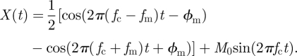
Signal analysis of the rat's locomotor activity allows us to cluster the data into three main groups: with one, two and three spectral components. We will show how the two spectral component case can be described as a linear superposition of two oscillators (zeitgeber and internal clock), whereas the three-component case can be described as a modulation of oscillators. In this latter case, the nonlinear interaction between the zeitgeber and an internal clock leads to modulation effects similar to that of radio signals. In fact, both amplitude modulation (AM) and frequency modulation (FM) lead to a spectra of three components similar to that in figure 2b. To illustrate this basic modulation principle, we focus here on AM. The one- and two-spectral component cases will be discussed later in this section. We start by connecting classical signal analysis results to the observed rat locomotor patterns. In particular, we present here a circadian carrier wave under AM where the carrier wave might be regarded as the internal SCN oscillator and the modulation wave emerges from an interaction between the zeitgeber and the internal clock. For the sake of simplicity, we assume that each involved rhythm has a sinusoidal waveform. A carrier wave C(t) and a modulation wave M(t) can be described as functions C(t) = C sin(2πf_ct + ϕ_c) + C₀ and M(t) = Msin(2πf_mt + ϕ_m) + M₀, respectively. Here, we set ϕ_c = C₀ = 0 and C = M = 1 and discuss the general case in the electronic supplementary material. An amplitude-modulated wave is obtained from the product X(t) = M(t)C(t). Using simple trigonometric identities we obtain:

4.1

Thus, the modulated signal X(t) has three spectral components, a main carrier wave of frequency f_c and two other waves (known as sidebands) whose frequencies are above and below the carrier frequency, i.e. f_l < f_c < f_h with the low frequency f_l = f_c − f_m and the high frequency f_h = f_c + f_m. The carrier period is τ_c = 1/f_c, the slow component period is τ_s = 1/f_l and the fast component period is τ_f = 1/f_h. Note that the sidebands are symmetric in the frequency spectrum and slightly asymmetric in the period domain. Analysis of the rat locomotor activity plotted in figure 2b presents a typical modulation-like spectrum with a circadian carrier wave and two smaller sidebands. Thus in this case, we can regard the SCN output as an amplitude-modulated signal. The theory predicts that both sidebands should be located at equal distances (in the frequency spectrum) from the carrier frequency. This implication can be tested using two of the observed components to predict the location of the third one. For example, using the experimentally measured periods of the main peak (carrier) and the fast component, it is possible to calculate the period of the slow component and the period of the modulation. In figure 2b, the carrier period is τ_c≃24.67 h and the fast component period is τ_f≃22.02 h. Using the relations described above in terms of the periods, i.e. τ_m = (1/τ_f − 1/τ_c)⁻¹ and τ_s = (1/τ_c − 1/τm)⁻¹, we obtain a modulation period of τ_m = 205 h and a predicted slow component of τ_s-predicted = 28.04 h. This coincides with the observed spectral peak at 28 h. Consequently, assuming modulation allows us to calculate the modulation period and the slow component period using two of the experimentally measured components.

In figure 3a, we sketch a circadian signal being amplitude modulated by a much slower wave resulting in a modulated X(t). In figure 3b, we use the expression of the modulated wave X(t) described by equation (4.1), plot its actogram and analyse its spectral components (figure 3c). Note that figure 3b,c results directly from a modulated circadian oscillation X(t) using two parameters from experimental data: τ_m = 205 h and τ_c = 24.64 h. Similar symmetrical sidebands and carrier wave are obtained by FM as illustrated in figure 3d–f. A frequency-modulated wave is obtained from X(t) = C sin(2πf_ct + M(t)). In this pure FM case there is no amplitude variations and thus the actograms look different. Nevertheless, the presence of two locomotor rhythms (highlighted in red and green) can be observed in both actograms and lead to almost identical spectra. Both AM and FM lead to the same symmetrical sideband frequencies with the low f_l = f_c − f_m and the high frequency f_h = f_c + f_m bands. Figure 3a–f illustrates that AM and/or FM reproduce the spectra observed in the forced desynchronization experiments.

Figure 3.

Modulation and linear superposition of waves with their associated actogram and spectral components. (a) Sketch of the AM with a circadian carrier wave C(t) being amplitude-modulated (AM) by a slow modulation M(t) resulting in an output wave X(t) = M(t)C(t). (b) Actogram of X(t) with the fast (shaded in red) and carrier (shaded in green) components and (c) the spectral components of such actogram. (d) FM of a circadian carrier wave C(t) under a slow FM M(t). The output wave is X(t) = C sin(2πf_ct + ϕ_c + M(t)). (e) Actogram of X(t) with the fast (shaded in red) and carrier (shaded in green) components and (f) the spectral components of such actogram. (g) Linear superposition of a circadian internal wave I(t) and the zeitgeber wave Z(t) resulting in an output wave X(t) = I(t) + Z(t). (h) Actogram of X(t) with the fast (shaded in red) and slow (shaded in green) components and (i) the spectral components of such actogram. For the AM plots in a–c we plot equation (4.1) with τ_m = 205 h, ϕ_m = π, M₀ = 0.2, τ_c = 24.6 h and modulation amplitude M = 0.3. For the FM plots in d–f we use τ_m = 205 h, ϕ_m = π, M₀ = 0.2, τ_c = 24.6 h and modulation amplitude M = 1. For the linear superposition plots in g–i we use T = 22 h, τ = 24.6 h and both amplitudes are set to 1.

In figure 3g–i, we illustrate the case of superposition of waves without modulation. A linear superposition of waves is obtained from X(t) = Z(t) + I(t) = B sin((2π/T)t) + I sin((2π/τ)t)) with B, T, I and τ as zeitgeber strength, period, internal amplitude and internal period, respectively. Two added circadian signals also lead to an actogram with two locomotor rhythms (highlighted in red and green in figure 3h) but in this case only two spectral components are present in the spectra (figure 3i). We will return to the linear superposition case when discussing the two spectral components group.

In order to provide further evidence of modulations, we pursue in figure 4 a similar strategy as for figure 2b: we analyse the activity data of all 21 rats, measure their locomotor activity spectral components and, if suitable, use two of the significant peaks to predict the period of a third component. From the 21 rats, seven rats show three circadian periods (figure 4), 10 show only two circadian periods (figure 5) and the rest shows only one significant period (figure 5a,b). Note that from the 21 rats studied in these experiments only 17 rats undergo forced desynchronization (show more than one peak in the spectrum) and one rat was discarded from the analysis owing to technical problems (rat 8). The three-component cases are presented in figure 4, where each plot represents the spectrum of a different rat with the fast, carrier and slow component periods depicted. The maximum power was normalized to 1 in each case. For each plot in figure 4, we use two measured components (bold numbers in figure 4) to predict the value of the third component period sketched by a vertical line in the spectra and annotated as the ‘predicted period’. We repeat this procedure three times per plot, i.e. we use the slow and fast to predict the carrier component, the fast and carrier to predict the slow component and the slow and carrier to predict the fast component. In all cases the predicted third peak is in good agreement with the experimentally measured value. Note that the relative power of each component is related to the amplitudes and phases of the carrier and modulation waves (see the electronic supplementary material) and in this part, we focus only on the periods.

Figure 4.

Spectral components of locomotor activity from seven rats maintained in a symmetric 22 h LD cycle. These rats are probably undergoing an AM and/or FM modulation and thus exhibit symmetrical sidebands. As a simple test in each subfigure we use two peaks (bold numbers) to predict the period of the third component sketched by a vertical line and annotated as ‘predicted value’. We repeat this procedure three times per plot: we use the slow and fast to predict the carrier component, the fast and carrier to predict the slow component and the slow and carrier to predict the fast component. See §9 for experimental and data analysis details.

Figure 5.

Spectral components of locomotor activity from 13 rats maintained in a symmetric 22 h LD cycle. (a) Two rats presumably inside the entrainment region with only one component coinciding with the 22 h zeitgeber period. (b) One rat seems to be unperturbed by the LD cycle and exhibits a rhythm close to the free running period. (c–f) Most of the rats under forced desynchronization showed two locomotor peaks, i.e. a 22 h zeitgeber component and a ca 25 h component similar to the measured internal period. See §9 for experimental and data analysis details. (a) Solid line, rat 4; dotted line, rat 15. (d) Solid line, rat 4; dotted line, rat 16; dashed line, rat 21; dashed-dotted, rat 13. (e) Solid line, rat 12; dotted line, rat 18; dashed line, rat 20. (f) Solid line, rat 14; dotted line, rat 1.

Altogether, these results suggest a strong correlation of the three main circadian peaks of the rats' locomotor activity, which can be explained as a slow AM and/or FM of the clock output. This modulation follows a much slower time scale with a period around 205 h (8 days).

Following an anonymous reviewer's suggestion, we analysed the spectral components of the locomotor activity of 21 rats under free-running conditions (constant darkness) and under 24 h LD (T24) entrainment cycles (data not shown). We found no evidence of sidebands in these data and, thus, we conclude that the sidebands observed here are specific for rats undergoing forced desynchronization.

In figure 5, we present the spectral analysis of the remaining rats under the T22 LD cycle. Similar spectra are grouped in the same graph, for instance figure 5e contains the spectra of the activity of rats 18, 12 and 15. Remarkably, under these challenging entrainment conditions two animals (rat 5 and rat 15) were able to entrain (figure 5a) and consequently the spectra exhibit only one circadian component at the zeitgeber period as the examples in figure 1g–i. On the other hand, one rat locomotor activity (rat 10) seems unperturbed by the external zeitgeber and shows only one circadian period similar to the expected free-running period (figure 5b). All the other rats have a two-component spectra (figure 5c–f). The fast period component coincides with the zeitgeber period around 22 h and the slow component with the internal or free running period as measured in Campuzano et al. [8]. These two-component cases can be simply described as a linear superposition of two waves as depicted in figure 3g–i and discussed in Wever [23] and Linkens [24].

In the following sections, we will see how the presence of a slow rhythm is in fact a generic feature of oscillators near the entrainment region and how this leads to patterns exhibiting one, two and three spectral components.

5. Slow oscillations emerge at the borderline of entrainment regions

The results of the three-component case discussed in §4 strongly suggest slow AM or/and FM rhythms acting on the circadian clock. The biological mechanism generating such slow oscillations are not known yet. In this section, we identify a likely dynamical origin of such slow rhythms.

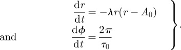
When an oscillator is near its entrainment region, a slow modulation can appear. This is a well-characterized generic phenomenon of oscillators observed in biology, physics and chemistry [25,26] and was already reported under forced desynchronization studies where melatonin release exhibits a slow modulation [17]. Slow modulations have been classified into two groups depending on whether a beating effect or a modulation phenomenon dominates. Beating is characterized by a linear superposition of two oscillations, whereas modulation phenomena reflect more complicated interactions between the oscillators leading to AM and/or FM [23,24]. Note that these phenomena were associated with terms such as ‘relative coordination’, ‘oscillatory free-run’ and ‘relative entrainment’ [23]. Here, we stay with a description derived from the theory of coupled oscillators that provides a well-defined framework to describe phenomena outside the entrainment range. For illustrative purposes we use a generic model oscillator to study in detail how slow periods arise from out-of-entrainment phenomena. Our generic oscillator model is characterized only by its amplitude, period and its stability with respect to amplitude perturbations (amplitude relaxation rate or Floquet exponent [27]). These general oscillator properties are conveniently parametrized by the Poincaré oscillator [28], which is given by the following equations in polar coordinates with the radial coordinate r and phase ϕ:

5.1

Here, A₀ and τ₀ denote the amplitude and intrinsic period of the oscillator. The parameter λ quantifies the relaxation of amplitudes to the stable oscillation (limit cycle) at r = A₀.

In Cartesian coordinates this oscillator has two oscillatory state variables, i.e. horizontal X(t) and vertical Y(t). The entrainment signal (zeitgeber), applied to oscillator's horizontal coordinate, is considered as a simple sinusoidal function Z(t) = B sin((2π/T)t) with B and T the zeitgeber strength and period, respectively (see §9 for details). In figure 6, we present a numerical and theoretical study of a circadian oscillator near the entrainment region. We study a self-sustained 24 h oscillator driven by short zeitgeber periods. The horizontal coordinate X(t) is considered as the output of the oscillator (figure 6a,b). An oscillator can leave its entrainment region by challenging zeitgeber periods and/or strength (figure 1b). Independent of which zeitgeber parameter is varied, there are two generic dynamical routes by which an oscillator loses entrainment, a saddle-node (SN) bifurcation of limit cycles and a Hopf bifurcation [26]. In both cases a slow oscillation close to the entrainment region arises. Interestingly, one way leads to beating and the other to modulations. We start here with modulations and discuss in the next sections both mechanisms in detail. We choose the zeitgeber strength such that the lower limit of entrainment is around 23 h and study the out-of-entrainment dynamics for zeitgeber periods ranging from 23 to 21 h (circles 1–5 in figure 6b). Inside the entrainment region the oscillator has a stable phase and amplitude but outside this region both phase and amplitude change in time. Close to the border of entrainment, the amplitude of the oscillator exhibits extremely slow variations. The period of such a modulation can be calculated as the time between the highest peaks of the AM (figure 6a). We present the results in figure 6c where the triangles represent the numerically calculated and the solid black line the analytical results (see the electronic supplementary material for the analytic derivation). At the border of entrainment the modulation period tends to infinity and decays for zeitgeber periods further away from the entrainment border.

Figure 6.

Generic behaviour of an oscillator outside the entrainment region where a slow modulation appears. (a) A circadian oscillator forced with short zeitgeber periods out of the entrainment region. The oscillator state variable X(t) is taken as the oscillator output with modulation. (b) Schematic of the oscillator entrainment region as a function of the zeitgeber period and amplitude. Here, the zeitgeber strength is such that the lower limit of entrainment is ca 23 h. (c) Numerical and analytical calculation of the modulation period as a function of the zeitgeber period. Blue filled triangles, simulation; solid line, theory. We numerically simulate the generic oscillator described in equation (5.1) with A₀ = 1, λ = 1 and τ₀ = 24. In §9 and the electronic supplementary material further analytical and numerical details are given.

As discussed, such slow modulations lead to symmetrical sidebands as experimentally observed in figures 2b and 4 and theoretically described in figure 3a–f. The slow modulation period depends on the zeitgeber period and, consequently, the carrier and sideband components will also vary with the zeitgeber period. In §§6 and 7, we compare quantitative results of our model with the data described in Campuzano et al. [8] (figure 2c,d).

Note that our model based on one driven self-sustained oscillator is not in contradiction with previous interpretations based on two oscillators [9,17,11]. A driven oscillator implies the presence of two oscillators, i.e. a driver and a driven oscillator. One subgroup of cells within the SCN might oscillate with the external 22 h, and another group might represent the autonomus oscillations. We show here that a model based on only one driven oscillator is sufficient to describe the observed complex patterns.

6. Modulation of a circadian oscillator

We have shown that signal analysis of rats' locomotor activity data reveals slow modulations in seven of the 17 rats undergoing forced desynchronization. In §5, we discussed how such slow modulations emerge as a generic behaviour of oscillators out-of-entrainment and how its period varies. The varying modulation period leads to specific temporal patterns. In figure 7, we characterize such patterns in terms of time series, actograms, phase evolution and spectral components. The patterns are studied in our generic oscillator model for four different zeitgeber periods. We choose here the zeitgeber strength such that the lower limit of entrainment is around 21.9 h. For a zeitgeber period of 22 h, the oscillator is still inside its entrainment region, no modulation occurs, the actogram shows the typical parallel stripes, the phase difference is stable and only one significant spectral component is present (figure 7d,h,l,p). The phase is numerically calculated as the phase difference between the oscillator state variable and the zeitgeber signal Z(t). Note that the oscillator takes around 15 days to achieve entrainment, i.e. stable phase, in agreement with the long transient times expected at the borders of the entrainment region [23,29].

Figure 7.

Circadian oscillator undergoing modulation outside the entrainment region. Time series of the oscillator state variable, actograms, phase evolution and spectral analysis of a periodically driven oscillator. We study the oscillator state variable under challenging short sinusoidal entrainment signals (from 22 to 20 h). For zeitgeber periods shorter than 22 h the oscillator exhibits modulation and sidebands appear in the spectra. (a–d) Time series of the oscillator state variable and (e–h) the associated 24 h actogram plots. (i–l) Normalized phase difference evolution as a function of time measured in zeitgeber cycles units. Long epochs of almost constant phase and short epochs of rapidly changing phase are known as phase slips (k). (m–p) Normalized power of the spectral components for different zeitgeber periods. See §9 for simulation details.

For periods shorter than 22 h the oscillator is out of its entrainment region, modulation appears and no parallel stripes are visible in the associated actogram (figure 7c,g,k,o). For such zeitgeber periods close to the border of entrainment there is no stable phase difference but a characteristic phase pattern. Long epochs of almost constant phase and short episodes of rapidly changing phase (figure 7k) are known as phase slips [26,30]. A spectral analysis reveals multiple components including a fast (dot), a carrier (square) and a slow component (diamond). For a shorter zeitgeber period of 21.25 h, the actogram can be interpreted as carring two rhythms: a shorter and a longer shaded in red and green, respectively (figure 7f). Nevertheless, a spectral analysis reveals three components: fast, carrier and slow component. This spectrum shows symmetrical sidebands and as a signature of AM and/or FM (compare figure 7n with figure 3a,b). Note that here the phase runs are unbounded and no phase slips occur (figure 7j). A similar pattern is observed for even shorter zeitgeber periods with the slow and fast components spreading further apart from the carrier period (figure 7a,e,i,m).

In order to compare our simulations with the experimental data shown in figure 2c,d, we plot in figure 8 the numerically and theoretically calculated slow, carrier and fast components for zeitgeber periods ranging from 20 to 23 h. Inside the entrainment region only one significant component is present, i.e. the oscillator state variable period is locked to the zeitgeber period. For shorter zeitgeber periods, the oscillator leaves the entrainment region crossing the lower limit of entrainment around 22 h and three spectral components diverge symmetrically (figure 8b). Assuming that the 24 h oscillator is undergoing modulation allows us to obtain an analytical expression for the fast and slow components in good agreement with the numerically calculated components (see the electronic supplementary material for the analytical derivation of sidebands). From a nonlinear dynamics point of view the patterns presented in figures 7 and 8 are closely related to an SN bifurcation of a limit cycle to a torus [26,30].

Figure 8.

Circadian spectral components of a circadian oscillator under modulation. (a) For zeitgeber periods shorter than 22 h this oscillator escapes from its entrainment region, exhibits modulation and sidebands appear in the spectra. The patterns presented here and in figure 7 are closely related to an SN bifurcation of a limit cycle to a torus. (b) Three main circadian spectral component periods for varying zeitgeber periods. We present both analytical (solid lines in blue, green and red represent theory) and numerical (squares, diamonds and circles in green, blue and red represent simulation, respectively) results. (c) Detailed view of the plot (b) with only the carrier and fast component for comparison with the results presented in figure 2c. (d) Normalized power of the three components for different zeitgeber periods. See §9 for simulation details.

For comparison with figure 2c, we plot in figure 8c only the carrier and fast component periods. Note that in both the measured rat locomotor activity and the simulations, the carrier component exhibits a small period decrease for a 2 h increase of the zeitgeber period. This slight period dependence on the external zeitgeber is known as frequency pulling [31]. Additionally, in simulation and experiments, the fast component follows the external zeitgeber period. Furthermore, we calculate the normalized power of the three main significant components for different zeitgeber periods (figure 8d). The fast and slow components show a similar pattern of their power: they have a maximum value close to the lower limit of entrainment followed by a monotonous decay for shorter zeitgeber periods. The carrier component is the main component for almost all zeitgeber periods. Our simulation results (figure 8d) and the experimental results (figure 2d) show similar trends but differences in details. Presumably additional parameters not considered in our simplified model affect sideband amplitudes (further discussion in the electronic supplementary material).

In §7, we present the alternative generic route by which an oscillator loses entrainment, termed beating mechanism.

7. Beating of a circadian oscillator

From the two generic routes by which an oscillator loses entrainment we discussed above the modulation mechanism. In this section, we characterize the patterns of a circadian oscillator losing entrainment by a beating mechanism. To illustrate the beating mechanism we use a beating-prone version of the original model oscillator achieved here by changing the amplitude relaxation rate parameter (see §9). The zeitgeber strength is the same as in figures 7 and 8. The beating emerges when the driven oscillator escapes from the entrainment region. For a zeitgeber period of 22 h, the oscillator is still inside its entrainment region, no beating is present, the stripes in the actogram show the typical positive slope, and there is a stable phase difference and only one significant spectral component (figure 9d,h,l,p).

Figure 9.

Circadian oscillator with beating. Time series of the oscillator state variable, actograms, phase evolution and spectral analysis of a periodically driven generic circadian oscillator. We study the oscillator state variable under challenging short sinusoidal entrainment signal (from 22 to 20 h). For zeitgeber periods shorter than 22 h the oscillator exhibits beating. (a–d) Time series of the oscillator state variable and (e–h) the associated 24 h actograms. (i–l) Phase difference evolution as a function of time measured in zeitgeber cycles units. (k) Periodically changing phase is known as phase trapping. (m–p) Normalized power of the spectral components for different zeitgeber periods. See §9 for simulation details.

For shorter periods, the oscillator is out of its entrainment region, beating appears, the associated actogram reveals a complex pattern and no parallel stripes are visible (figure 9c,g,k,o). For a zeitgeber close to the border of entrainment there is no stable phase difference but an oscillatory phase pattern. This periodically changing phase (figure 9k) is known as phase trapping [26,32]. For a shorter zeitgeber period of 20.5 h, the actogram shows steeper stripes and the phase runs unbounded (figure 7f,j). A spectral analysis of the time series outside entrainment reveals two components: a fast (dot) and a carrier (square) component. The fast component follows the external zeitgeber and the carrier component expresses the internal period of the oscillator, i.e. 24 h in our model. These spectra with two bands, internal and zeitgeber, is a characteristic of beating (compare with figure 3i). For shorter zeitgeber periods, the internal component increases its power. Thus the stripes become steeper approaching the vertical stripes pattern of a 24 h rhythm actogram (figure 1d).

In figure 10, we follow the beating period and both spectral components as the zeitgeber period is reduced. Here, the lower limit of entrainment is around 21 h (see figure 10a and §9 for model details). As in the modulation case, a slow oscillation emerges outside the entrainment region. This slow rhythm, called beating, has its own dynamical signatures that we describe below. The beating period is numerically calculated as the time between the highest peaks of the amplitude variations (as sketched in figure 6a). There is no period divergence at the border of entrainment (figure 10b). In signal analysis, beating is characterized as a linear superposition of two signals as shown in figure 10c. Here, the carrier component emerges at the border of entrainment with a stable period close to 24 h whereas the fast component follows independently the zeitgeber period. Inside the entrainment region, the normalized power of the unique carrier component decays as the oscillator approaches the border of entrainment. At the borderline both components have similar normalized power but for shorter zeitgeber periods the carrier component predominates and the fast component power decreases (figure 10b). From a nonlinear dynamics point of view, the patterns presented in figures 9 and 10 are closely related to a Hopf bifurcation of a limit cycle to a torus [26,30].

Figure 10.

Circadian spectral components of a circadian oscillator undergoing beating. (a) For zeitgeber periods shorter than 21 h this oscillator escapes from its entrainment region and exhibits beating and only two components appear in the spectra. The patterns presented here and in figure 9 are closely related to a Hopf bifurcation of a limit cycle to a torus. (b) Numerical calculation of the beating period as a function of the zeitgeber period. (c) Two main circadian spectral components for increasing zeitgeber periods. (d) Normalized power of the two components for different zeitgeber periods. See §9 for simulation details.

Note that from dynamical systems theory, it is known that a set of synchronized coupled oscillators can be described as a one-oscillator model where the parameters and variables represent the whole synchronized population. Thus, the results obtained in this and the previous sections studying one generic oscillator are general enough to apply to either single cells, or a synchronized rhythm generated by a set of coupled oscillators.

8. Concluding remarks

In this paper, we demonstrate how the rich activity patterns of rats undergoing forced desynchronization can be consistently explained in terms of only one driven oscillator. We show how the data clustered into two groups. One group exhibiting two independent spectral components, described as a linear superposition of waves, related to a beating mechanism and showing characteristic dynamical signatures of a Hopf bifurcation. The other group has three spectral components, a central carrier wave and two symmetrical sidebands, and can be described as a modulation of waves. This group has characteristic dynamical signatures of an SN bifurcation. The remaining rats do not exhibit forced desynchronization, i.e. their activities have only one circadian spectral component, and might be either inside or far away from the entrainment zone.

Previous studies interpreted the forced desynchronization results as an in vivo dissociation of two neural subpopulations within the SCN. Our results indicate that a single driven oscillator can explain the data. Nevertheless, our results are not in contradiction with previous interpretations based on two oscillators. A subpopulation of neurons such as the ventrolateral SCN might follow the driving LD cycle and another group of neurons could represent the autonomous oscillator. Interactions of these populations might lead to the observed modulations with sidebands. Further studies are necessary to investigate the biological mechanisms behind modulations.

Throughout this paper, we provide a framework that combines signal analysis and the theory of oscillators for the study of circadian desynchronization. Future studies might take this work as an starting point.

9. Material and methods

9.1. Analysis of locomotor activity

In this paper, we analysed the data of a total of 21 rats under square-wave cycles of 22 h (11 h light, 11 h dark). Two-month-old male Wistar rats were housed individually in 25 × 25 × 12 cm transparent cages, and their motor activities were recorded with crossed infrared beams, as described previously [8,9,33]. The original raw activity is available by request to the authors and is organized as follows: column 1 refers time in minutes, columns 2–22 refer to locomotor activity of rats 1–21. We group the rat's activity data based on the number of peaks observed in the spectra within the range of 20–30 h. The selection was based on three different spectral analysis methods: Sokolove & Busshell periodogram [34], Chi-square Clocklab data analysis tool and Matlab in-built function ‘periodogram.m’. The spectral analysis used for the figures was done with Matlab in-built function ‘periodogram.m’ applied directly to the raw activity data without noise filter or data window. By dividing each spectrum by its maximum peak, we obtained a normalized power spectral density. For the spectral analysis initial activity days were discarded because of transients and failures in the detection system: in figure 4 we discarded the first 5 days for all rats except for rats 17 and 19 were we discard the first 15 days. For figure 5 the first 10 days of activity of each rat were discarded from the analysed data. Figure 2c,d is adapted from Campuzano et al. [8]. In this series of experiments, six groups of eight rats each were exposed to a symmetric LD cycle with periods of 21, 21.5, 22, 22.5, 23 and 23.5 h. In all cases, ‘light’ consisted of cool white light of 300 lux and ‘dark’ of dim red light of less than 0.5 lux. Animals were kept under these LD conditions for 60 days [8].

9.2. Oscillator model

The simulations were designed to illustrate the out-of-entrainment dynamics and depend on a few generic parameters that are representative for a large class of oscillators. Results presented in figures 1c–j, 6c, 7, 8b–d, 9 and 10b–d were numerically calculated using a forced Poincaré oscillator in Cartesian coordinates:

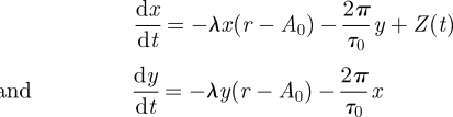The parameters represent the oscillator period τ₀, amplitude A₀ and amplitude relaxation rate λ. Introducing the radius r = (x + y)^1/2 and ϕ = arctan(y/x) leads to our model in equation (5.1). The oscillator is entrained by a forcing term acting on the horizontal coordinate Z(t) = B sin((2π/T)t) with B and T the zeitgeber strength and period, respectively. Without forcing, the oscillator has a 24 h period, i.e. τ₀ = 24 h and an amplitude of 1, i.e. A₀ = 1. For a moderate zeitgeber strength the Poincaré oscillator can exhibit modulation or beating. For figures 6–8 we use λ = 1 and for figures 9 and 10 we use λ = 0.03. For a moderate zeitgeber strength, this parameter modification from λ = 1 to λ = 0.03 change the bifurcation from a saddle node to a Hopf bifurcation and consequently from a modulation-prone to a beating-prone oscillator. Such bifurcation change can be also achieved by other parameter variations as discussed in detail in Balanov et al. [26].

In figures 1a, 6b, 8a and 10a, we sketched the 1 : 1 Arnold tongues of the Poincaré oscillator. A comprehensive bifurcation analysis of the Poincaré oscillator is out of the scope of this publication. In figure 6c, we choose the zeitgeber strength such that the lower limit of entrainment is around 23 h, i.e. B = 0.02, and for figures 7–10 we use a zeitgeber strength B = 0.05.

References

- 1.Welsh D. K., Logothetis D. E., Meister M., Reppert S. M. 1995. Individual neurons dissociated from rat suprachiasmatic nucleus express independently phased circadian firing rhythms. Neuron 14, 697–706 10.1016/0896-6273(95)90214-7 (doi:10.1016/0896-6273(95)90214-7) [DOI] [PubMed] [Google Scholar]
- 2.Westermark P. O., Welsh D. K., Okamura H., Herzel H. 2009. Quantification of circadian rhythms in single cells. PLoS Comput. Biol. 5, e1000580. 10.1371/journal.pcbi.1000580 (doi:10.1371/journal.pcbi.1000580) [DOI] [PMC free article] [PubMed] [Google Scholar]
- 3.Plano S. A., Golombek D. A., Chiesa J. J. 2010. Circadian entrainment to light–dark cycles involves extracellular nitric oxide communication within the suprachiasmatic nuclei. Eur. J. Neurosci. 31, 876–882 10.1111/j.1460-9568.2010.07120.x (doi:10.1111/j.1460-9568.2010.07120.x) [DOI] [PubMed] [Google Scholar]
- 4.Shirakawa T., Honma S., Honma K. 2001. Multiple oscillators in the suprachiasmatic nucleus. Chronobiol. Int. 18, 371–387 10.1081/CBI-100103962 (doi:10.1081/CBI-100103962) [DOI] [PubMed] [Google Scholar]
- 5.Aton S. J., Herzog E. D. 2005. Come together, right … now: synchronization of rhythms in a mammalian circadian clock. Neuron 48, 531–534 10.1016/j.neuron.2005.11.001 (doi:10.1016/j.neuron.2005.11.001) [DOI] [PMC free article] [PubMed] [Google Scholar]
- 6.Welsh D. K., Takahashi J. S., Kay S. A. 2010. Suprachiasmatic nucleus: cell autonomy and network properties. Annu. Rev. Physiol. 72, 551–577 10.1146/annurev-physiol-021909-135919 (doi:10.1146/annurev-physiol-021909-135919) [DOI] [PMC free article] [PubMed] [Google Scholar]
- 7.Vilaplana J., Cambras T., Campuzano A., Díez-Noguera A. 1997. Simultaneous manifestation of free-running and entrained rhythms in the rat motor activity explained by a multioscillatory system. Chronobiol. Int. 14, 9–18 10.3109/07420529709040537 (doi:10.3109/07420529709040537) [DOI] [PubMed] [Google Scholar]
- 8.Campuzano A., Vilaplana J., Cambras T., Díez-Noguera A. 1998. Dissociation of the rat motor activity rhythm under T cycles shorter than 24 h. Physiol. Behav. 63, 171–176 10.1016/S0031-9384(97)00416-2 (doi:10.1016/S0031-9384(97)00416-2) [DOI] [PubMed] [Google Scholar]
- 9.de la Iglesia H. O., Cambras T., Schwartz W. J., Dez-Noguera A. 2004. Forced desynchronization of dual circadian oscillators within the rat suprachiasmatic nucleus. Curr. Biol. 14, 796–800 10.1016/j.cub.2004.04.034 (doi:10.1016/j.cub.2004.04.034) [DOI] [PubMed] [Google Scholar]
- 10.Cambras T., Chiesa J., Araujo J., Díez-Noguera A. 2004. Effects of photoperiod on rat motor activity rhythm at the lower limit of entrainment. J. Biol. Rhythms 19, 216–225 10.1177/0748730404264201 (doi:10.1177/0748730404264201) [DOI] [PubMed] [Google Scholar]
- 11.Schwartz M. D., Congdon S., de la Iglesia H. O. 2010. Phase misalignment between suprachiasmatic neuronal oscillators impairs photic behavioral phase shifts but not photic induction of gene expression. J. Neurosci. 30, 13 150–13 156 10.1523/JNEUROSCI.1853-10.2010 (doi:10.1523/JNEUROSCI.1853-10.2010) [DOI] [PMC free article] [PubMed] [Google Scholar]
- 12.Shinohara K., Honma S., Katsuno Y., Abe H., Honma K. 1995. Two distinct oscillators in the rat suprachiasmatic nucleus in vitro. Proc. Natl Acad. Sci. USA 92, 7396–7400 10.1073/pnas.92.16.7396 (doi:10.1073/pnas.92.16.7396) [DOI] [PMC free article] [PubMed] [Google Scholar]
- 13.Schwartz W. J. 2009. Circadian rhythms: a tale of two nuclei. Curr. Biol. 19, R460–R462 10.1016/j.cub.2009.04.044 (doi:10.1016/j.cub.2009.04.044) [DOI] [PubMed] [Google Scholar]
- 14.Canal-Corretger M. M., Cambras T., Vilaplana J., Díez-Noguera A. 2003. The manifestation of the motor activity circadian rhythm of blinded rats depends on the lighting conditions during lactation. Chronobiol. Int. 20, 441–450 10.1081/CBI-120021442 (doi:10.1081/CBI-120021442) [DOI] [PubMed] [Google Scholar]
- 15.Cambras T., Weller J. R., Anglès-Pujoràs M., Lee M. L., Christopher A., Díez-Noguera A., Krueger J. M., de la Iglesia H. O. 2007. Circadian desynchronization of core body temperature and sleep stages in the rat. Proc. Natl Acad. Sci. USA 104, 7634–7639 10.1073/pnas.0702424104 (doi:10.1073/pnas.0702424104) [DOI] [PMC free article] [PubMed] [Google Scholar]
- 16.Lee M. L., Swanson B. E., de la Iglesia H. O. 2009. Circadian timing of REM sleep is coupled to an oscillator within the dorsomedial suprachiasmatic nucleus. Curr. Biol. 19, 848–852 10.1016/j.cub.2009.03.051 (doi:10.1016/j.cub.2009.03.051) [DOI] [PMC free article] [PubMed] [Google Scholar]
- 17.Schwartz M. D., Wotusa C., Liub T., Friesenc W. O., Borjiginb J., Odad G. A., de la Iglesiaa H. O. 2009. Dissociation of circadian and light inhibition of melatonin release through forced desynchronization in the rat. Proc. Natl Acad. Sci. USA 106, 17 540–17 545 10.1073/pnas.0906382106 (doi:10.1073/pnas.0906382106) [DOI] [PMC free article] [PubMed] [Google Scholar]
- 18.Berge P., Pomeau Y., Vidal C. 1984. Order within chaos: towards a deterministic approach to turbulence. New York, NY: Wiley-Interscience [Google Scholar]
- 19.Takahashi J. S., Hong H.-K., Ko C. H., McDearmon E. L. 2008. The genetics of mammalian circadian order and disorder: implications for physiology and disease. Nat. Rev. Genet. 9, 764–775 10.1038/nrg2430 (doi:10.1038/nrg2430) [DOI] [PMC free article] [PubMed] [Google Scholar]
- 20.Ralph M. R., Foster R. G., Davis F. C., Menaker M. 1990. Transplanted suprachiasmatic nucleus determines circadian period. Science 247, 975–978 10.1126/science.2305266 (doi:10.1126/science.2305266) [DOI] [PubMed] [Google Scholar]
- 21.Silver R., LeSauter J., Tresco P. A., Lehman M. N. 1996. A diffusible coupling signal from the transplanted suprachiasmatic nucleus controlling circadian locomotor rhythms. Nature 382, 810–813 10.1038/382810a0 (doi:10.1038/382810a0) [DOI] [PubMed] [Google Scholar]
- 22.Reppert S. M., Weaver D. R. 2002. Coordination of circadian timing in mammals. Nature 418, 935–941 10.1038/nature00965 (doi:10.1038/nature00965) [DOI] [PubMed] [Google Scholar]
- 23.Wever R. 1972. Virtual synchronization towards the limits of the range of entrainment. J. Theor. Biol. 36, 119–132 10.1016/0022-5193(72)90181-6 (doi:10.1016/0022-5193(72)90181-6) [DOI] [PubMed] [Google Scholar]
- 24.Linkens D. A. 1979. Theoretical analysis of beating and modulation phenomena in weakly inter-coupled van der Pol oscillator systems for biological modelling. J. Theor. Biol. 79, 31–54 10.1016/0022-5193(79)90255-8 (doi:10.1016/0022-5193(79)90255-8) [DOI] [PubMed] [Google Scholar]
- 25.von Holst E. 1939. Die relative Koordination als Phaenomen und als Methode zentralnervoeser Funktionsanalyse, vol. 42 Berlin, Germany: Springer [Google Scholar]
- 26.Balanov A., Janson N., Postnov D., Sosnovtseva O. 2009. Synchronization: from simple to complex. New York, NY: Springer [Google Scholar]
- 27.Guckenheimer J., Holmes P. 1983. Nonlinear oscillations, dynamical systems, and bifurcations of vector fields. New York, NY: Springer [Google Scholar]
- 28.Glass L., Mackey M. C. 1988. From clocks to chaos: the rhythms of life. Princeton, NJ: Princeton University Press [Google Scholar]
- 29.Granada A. E., Herzel H. 2009. How to achieve fast entrainment? The timescale to synchronization. PLoS ONE 4, e7057. 10.1371/journal.pone.0007057 (doi:10.1371/journal.pone.0007057) [DOI] [PMC free article] [PubMed] [Google Scholar]
- 30.Pikovsky A., Rosenblum M., Kurths J. 2001. Synchronization: a universal concept in nonlinear sciences. Cambridge, UK: Cambridge University Press [Google Scholar]
- 31.Linkens D. A. 1979. Modulation analysis of forced non-linear oscillators for biological modelling. J. Theor. Biol. 77, 235–251 10.1016/0022-5193(79)90356-4 (doi:10.1016/0022-5193(79)90356-4) [DOI] [PubMed] [Google Scholar]
- 32.Aronson D. G., Ermentrout G. B., Kopell N. 1990. Amplitude response of coupled oscillators. Physica D: Nonlinear Phenomena 41, 403–449 10.1016/0167-2789(90)90007-C (doi:10.1016/0167-2789(90)90007-C) [DOI] [Google Scholar]
- 33.Cambras T., Vilaplana J., Campuzano A., Canal-Corretger M. M., Carulla M., Díez–Noguera A. 2000. Entrainment of the rat motor activity rhythm: effects of the light–dark cycle and physical exercise. Physiol. Behav. 70, 227–232 10.1016/S0031-9384(00)00241-9 (doi:10.1016/S0031-9384(00)00241-9) [DOI] [PubMed] [Google Scholar]
- 34.Sokolove P. G., Bushell W. N. 1978. The chi square periodogram: its utility for analysis of circadian rhythms. J. Theor. Biol. 72, 131–160 10.1016/0022-5193(78)90022-X (doi:10.1016/0022-5193(78)90022-X) [DOI] [PubMed] [Google Scholar]