Balance equations can buffer noisy and sustained environmental perturbations of circadian clocks

Abstract

We present a new approach to understanding how regulatory networks such as circadian clocks might evolve robustness to environmental fluctuations. The approach is in terms of new balance equations that we derive. We use it to describe how an entrained clock can buffer the effects of daily fluctuations in light and temperature levels. We also use it to study a different approach to temperature compensation where instead of considering a free-running clock, we study temperature buffering of the phases in a light-entrained clock, which we believe is a more physiological setting.

1. Introduction

Circadian oscillators are entrained by the daily cycles of light and temperature. It is therefore important that a clock is sensitive to their daily periodicity. On the other hand, there are very substantial stochastic day-to-day fluctuations in these environmental cycles. This can, for example, be seen in the time series for light intensity and temperature shown in figures 1 and 2. The daily fluctuations in both are substantial: the fluctuations in light have a coefficient of variation of approximately 36 per cent, while those of England's maximum and minimum temperatures in degrees centigrade over just the single month of September have a coefficient of variation 15 and 29 per cent, respectively.

Figure 1.

Light intensity measurements for the month of September 2005 from the environmental radiometry data from Harvard Forest [17].

Figure 2.

Daily maximum and minimum temperature measurements for the month of September 2005 from UK Met Office Historical Central England data (HadCET) [18].

The presence of such substantial noisy perturbations raises a number of questions. Our theoretical understanding suggests that in a typical model these perturbations will produce substantial fluctuations in the protein levels (e.g. figure 4). This seems to be in conflict with the need for the clock to provide robust signals to the genes that it is controlling. It therefore raises the question of whether the clock can be designed so that the daily protein variation is robustly entrained but at the same time the system manages to effectively buffer the stochastic variations.

Figure 4.

Effect of light intensity fluctuations on the protein profile of the morning loop component LHY of the Locke model. The profile reflects levels of the cytoplasmic protein for light intensity α ∼ 𝒩(1,0.2).

In this paper, we explain how it is relatively easy for evolution to adjust a clock network so as to carry out such buffering of stochastic environmental fluctuations. We argue that this is potentially an important reason why an oscillator, rather than a direct measurer of the entraining signal (light or temperature) is used. The mathematical argument that we employ is very general and can be applied to a much broader class of regulatory and signalling systems and other environmental factors. It uses a combination of ideas behind balance equations (used previously to explain temperature compensation [1–3]) and the principal component aspects of global sensitivity analysis [4–8]. We consider fluctuations in the light level and temperature fluctuations. To give examples of the effectiveness of the buffering mechanism for light fluctuations, we use a published model of the Arabidopsis thaliana circadian clock [7], and for temperature fluctuations, we introduce a temperature-dependent version of this model.

A related issue was addressed in a recent paper [8]. In a study involving artificial in silico evolution of clock networks, it was shown that a combination of the need to cope with multiple photoperiods and stochastic variation in the timing of dawn and dusk favoured the evolution of more loops and light inputs and greater complexity in the networks.

After considering short-term fluctuations, we turn to temperature compensation. Temperature compensation refers to the striking and defining feature of circadian clocks whereby their period only varies by a small amount over a physiological range of temperatures [9,10]. However, the exact value of the free-running period in constant conditions does not appear to have a direct selective value in the natural environment, as the clock will normally be entrained to diurnal day/night cycles. One may therefore ask why temperature compensation has arisen during evolution. We address this question here and develop a theory to address the question of how evolution might act on forced entrained oscillators. We show that for typical systems, the phases of the proteins in the clock will vary significantly with temperature but that one can tune the clock to satisfy certain balance equations so that the changes in phase are buffered. We propose that the buffering of the free-running period characteristic of classically temperature-compensated systems is a consequence of this phase buffering. The idea that there is a connection between the free-running period and the entrained phase is not a new one. The way in which phase changes as one crosses an Arnold tongue is well understood in dynamical systems theory [5,11] and in circadian rhythms [12,13]. This relation between the period and the entrainment phase has been observed experimentally in physiologically relevant situations [14].

Throughout, we assume that our circadian clock is modelled by a set of ordinary differential equations

1.1

where t is time, a vector x = (x₁, … , x_n) represents the state variables (namely, mRNA and protein levels) and k = (k₁, … , k_s) is a vector of parameter values. We assume that equation (1.1) has an attracting periodic solution x = g(t,k) of period T. We study the properties of this solution. We will illustrate our results by using a model of the Arabidopsis circadian clock [7].

2. Global sensitivity analysis and its principal components

If g(t) is the solution of equation (1.1) mentioned above, then the change δg(t) in g caused by a change δk = (δk₁, … , δk_s ) in the parameter vector k is

where the linear map M is given by

We can regard M as a map from the parameter space ℝ^s to a space of time series. For our purposes, the appropriate space of time series is the Hilbert space ℋ defined in appendix A, and we also consider the subspace ℋ₀ of ℋ spanned by the functions ∂g/∂k_j(t) on 0 ≤ t ≤ T, j = 1, … , s.

In Rand [6], it is shown that there are a set of numbers σ₁ ≥ σ₂ ≥ … ≥ σ_s, a set of orthonormal vectors V₁, … ,V_s of the parameter space ℝ^s and a set of orthonormal vectors U₁, … ,U_s in ℋ such that MV_i = σ_iU_i, M*U_i = σ_iV_i with the following optimality property: for all k ≥ 1, the average error given by

is minimized over all orthonormal bases of H₀. At this minimal value, e_k² = cσ_k², where c is an absolute constant. The σ_i are uniquely determined and the V_i and U_i are, respectively, eigenvectors of MM* and M*M. Thus, the σ_i are the eigenvalues of M*M. If they are simple eigenvectors, then the U_i and V_i are uniquely determined.

M* is the adjoint to M and is given by

where

It follows that the ijth element of M*M is given by

Since this is self-adjoint, it has real positive eigenvalues and these are σ₁ ≥ σ₂ ≥ … ≥ σ_s.

It follows from the above discussion that a change δk to the parameters leads to a change δg in the solution g such that

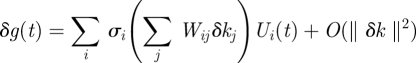and that the σ_i decay as rapidly as is possible for any such representation. Here, the W_ij are the elements of the inverse matrix W = V⁻¹. The speed with which the σ_i decay for the Arabidopsis clock model [7] is shown in figure 3. Inspection of figure 3 shows that this decay is exponential for the case for the clock model of Locke et al. [7], and this is typical [4,6,15] as also shown in the electronic supplementary material, figure S1.

Figure 3.

Plot of log₁₀(σ_i/σ₁) for the largest singular values of the clock model [9]. The σ_i decay exponentially.

Note that when applying this theory, one can either apply it directly to the model parameters k_j or one can apply it to the parameters η_j = log k_j. It is often more relevant to use the second approach because, in regulatory and signalling systems, the values of two parameters may differ by an order of magnitude or more. Therefore, it is more appropriate to consider relative changes in the parameters k_j than the absolute changes. The only change to the theory when considering relative changes instead of absolute ones is to replace the linear operator M above by M · Δ, where Δ = diag(k) is the diagonal matrix whose diagonal is made up of the parameter values. If we denote quantities for the latter relative case using a tilde, we have Ṽ = Δ · V, W̃_ij = k_jW_ij and σ̃_i = σ_i. This follows from the fact that for small changes δk to the model's parameters, δη_j = δk_j/k_j. The scaled changes δη_j also have the advantage of being non-dimensional.

3. Balance equations for sustained and daily fluctuations

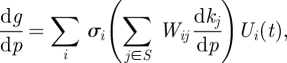
Now suppose that a subset {k_j1, … , k_jq} of the parameters depend upon a parameter p, i.e. k_jm = k_jm(p). Then,

3.1

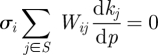
where the latter sum is over j in 𝒮 = {j₁, … , j_q}. Thus, if we want dg/dp = 0, we require

3.2

for i = 1, … , s. The s equations in (3.2) are called the balance equations and the sums ∑_j∈𝒮 W_ij dk_j/dp are called balance sums.

Note that the ith balance equation can only be solved if, for this value of i, the W_ijdk_j/dp do not all have the same sign. This places a constraint on the W_ij and hence on the system as a whole.

Now we come to the reason why using the above principal components U_i is important. Note that in equation (3.1), each term ∑_j∈S W_ijdk_j/dp is multiplied by σ_i and therefore if the σ_i decrease rapidly, as usually is the case for the sort of systems that we consider, then the importance of the balance equations in ensuring dg/dp ≈ 0 decreases rapidly as i increases, and obtaining the balance equations for just a few low i will substantially decrease |dg/dp|. Inspection of figure 3 shows that this is certainly the case for the clock model of Locke et al. [7] and this is typical [4,6,15].

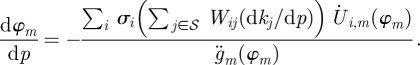
For circadian oscillators, we are often particularly interested in the changes in phase of the various components of the clock. If we define the phase φ_m of the mth component as the time that it reaches its maximum value, then [6]

3.3

A derivation of equation (3.3) is provided in appendix A. Thus, the balance equation to obtain dφ_m /dp ≈ 0 agrees with equation (3.2).

In practice, the balance sums are never zero, and the aim of the balancing is to reduce them substantially in the sense that the ratio of the sum after balancing to that before is substantially less than one.

4. Application to daily light fluctuations

Our aim here is to demonstrate a simple mechanism that can enable the clock to filter out the sort of substantial variation in daytime light intensity that is observed in the Harvard Forest data [17], figure 1.

We denote the time-dependent light intensity by θ(t). For example, θ(t) might be the function that is 1 between dawn t_l and dusk t_d and zero elsewhere or it might be a slightly smoothed version of this discontinuous function. We model fluctuations in the light by replacing θ(t) by αθ(t), where α fluctuates daily around its mean value of α = 1.

We then consider a model where the effect of light is to modulate a subset of the terms in the differential equation so that they are functions of αθ(t). In general, the light input will occur in multiple terms in the form k_jθ(t), where k_j is one of the parameters of the system. If the light level is fluctuating as above, then the term k_jθ(t) is replaced by k_jαθ(t). Let 𝒮 be the set of parameter indices for the parameters that occur in this way.

Suppose that this original model is not buffered against variation in daytime light intensity. To buffer it, we can assume that there is some simple regulation of the light inputs, so each of the terms k_jαθ(t), j ∈ 𝒮, is replaced by k_j(c_jα + d_j)θ(t). It is also natural to assume that c_j + d_j = 1 since this implies that k_j(c_jα + d_j) fluctuates around k_j. One can always reduce to this case by scaling the k_j in advance. We call this the light-modified model.

If c_j and d_j are fixed (and not regarded as parameters), then the new value for W_ij in this new system is c_jW_ij, where the latter W_ij is the value in the original system. Therefore, the balance equation for absolute changes in the parameters is

4.1

where the W̃_ij are as above for the approach where one uses relative changes in parameters instead of absolute ones so that one uses η_j = log k_j.

This is a very general formulation and is, for example, directly applicable to the model of Locke et al. [7] for the Arabidopsis clock that introduces light in the way described. The light parameters k_j, j ∈ 𝒮, are listed in table 1. The light parameters that have the greatest effect on the balance equations (by ranking σ_iW_ij) are LHY transcription (q₁), light and TOC1-mediated induction (q₂ and n₄) of Y transcription and accumulation of protein P (p₅).

Table 1.

Left: parameters for the balanced model. Each light parameter k_j has light intensity of the form α_jL(t). For the Locke model, α_j = α = 1, while for the balanced model, α_j = c_jα + d_j, where c_j are listed in the table and d_j are d_j = 1−c_j. Right: the sum ∑_jW_ijdk_j/dα for i = 1,…, 8 evaluated for the Locke model (dk_j/dα = 1) and the balanced model (dk_j/dα = c_j). The corresponding singular values σ_i are plotted in figure 3.

kj	cj	∑jεSWij (dkj/dα)
		i	(dkj/dα) = 1	(dkj/dα) = cj
q1	1.1918
n0	1.2	1	0.0002	−0
m5	−314.2308	2	0.0094	0
m7	1.0163	3	−0.0158	−0
q2	1.2491	4	0.0466	−0.0117
n4	−0.2427	5	−0.0213	0.0154
p5	−0.6042	6	−0.0453	0.0140
q3	1.5	7	0.0032	0.0033
q4	1.0198	8	−0.0314	0.0116

We assume that the variations α are normally distributed with mean μ and standard deviation σ, which we denote by α ∼𝒩(μ,σ). As shown in figure 4 (and in the electronic supplementary material, figure S2), the daily variation in the amplitude of the limit cycle solution of this model is substantial and quantitatively reflects the variation in the light amplitude. A light-modified model was constructed as described for which the left-hand sides of equation (4.1) are substantially smaller, as is given in table 1.

To implement this, the values of six of the c_j were chosen fairly arbitrarily but relatively close to one and then the remaining three were calculated by solving the linear balance equations corresponding to the first three principal components. Our balanced model shows less variation in the output protein and gene levels (figure 5 for α ∼ 𝒩(1,0.2)). For all genes and proteins, the balanced model shows less variation in the concentration levels than the unbalanced Locke model (electronic supplementary material, figure S3 and table S1). The phases of the balanced model show less variation for all components, except the LHY gene and proteins, which are of same order as those of the Locke model (electronic supplementary material, table S2).

Figure 5.

Effect of light intensity fluctuations on the morning loop protein LHY of the balanced model. The profile reflects levels of the cytoplasmic protein for light intensity α ∼ 𝒩(1,0.2).

5. Application to daily temperature fluctuations

We consider a model with fixed but differing day and night temperatures, T_D and T_N. Below, we derive a set of balance equations that eliminate the effects of temperature fluctuations.

We assume that the temperature enters the model through a set of parameters k_j, j ∈ 𝒮, which are temperature sensitive. A standard assumption for the temperature dependence of each of model parameters k_j is that it is similar to that for rate constants of chemical reactions and is described by the Arrhenius equation. This expresses the dependence of the rate constant k_j on the temperature T and activation energy E_j as k_j = A_j exp(−E_j/RT), where A_j is a constant specific to the individual parameter and R is the gas constant (8.314472 × 10⁻³ kJ mol⁻¹K⁻¹). In our case, we need to deal with the fact that we have different night and day temperatures and therefore we assume

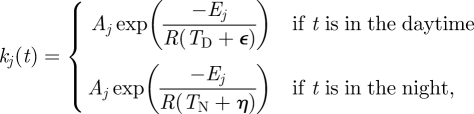5.1

where t is in the daytime if t_l ≤ t mod τ < t_d, where [t_l, t_d] denotes the range of day hours, and otherwise t is in the night. Moreover, ε and η denote the fluctuations in day and night temperatures, T_D and T_N, respectively. We consider the following first-order Taylor series expansion:

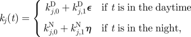5.2

where k_j,0^D = A_j exp(−E_j/RT_D) and k_j,1^D = − k_j,0^DE_j/RT_D and similarly for the night parameters. Note that this is a very good approximation and higher order terms can be neglected, since for a parameter of order 𝒪(0.1) (i.e. the order of a large number of Locke parameters), with sensible activation energy E ≈ 50 kJ mol⁻¹, the coefficient of the second-order term is of order 𝒪(0.001).

From the observation in equation (3.1), day temperature variations ε will have the following effects on changes to the solution g:

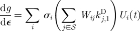5.3

and the following changes to the phases:

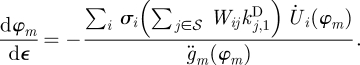5.4

Similar expressions can be derived for night temperature fluctuations. Together, these give rise to two sets of balance equations,

5.5

Or alternatively,

5.6

since, by the above, k_j,1^D = −k_j,0^DE_j/RT_D². In order to make a model temperature dependent, we have to define the dependence of its parameters on temperature. It is likely that all parameters in a regulatory system are actually temperature dependent, but this temperature dependence will have little effect for a parameter k_j if all the sensitivities S_ij = σ_iW_ij are small for that value of j. Therefore, in order to keep the model reasonably tractable, we will only introduce temperature into those variables with a significant sensitivity.

Moreover, to determine the relative importance of parameters, since values of some parameters differ by an order of magnitude or more, it is more appropriate to compare relative changes of parameters and to use the log parameters and the W̃_ij as described in the last paragraph of §2. We selected parameters that ranked highest when ordered by max_i=1−4 |σ_iW̃_ij|. The plot of top 20 is shown in figure 6. In this selection, we include only parameters that come linearly in the model and exclude Hill coefficients as these are not rate constants. Parameter n₆ has the highest max_i=1−4log₁₀|σ_iW̃_ij|. Only seven other parameters have sensitivity higher than 30 per cent of the maximum. These eight parameters will be temperature sensitive.

Figure 6.

Power sensitivity spectrum of the Locke model. Each group of bars corresponds to the values of log₁₀|σ_iW_ij| for a parameter k_j. These are only plotted for those i for which log₁₀|σ_iW_ij| is significant (here that is i = 1–4). The parameters k_j are ordered by max_i=1−4 log₁₀|σ_iW_ij| and only 20 most sensitive ones are plotted. Not taking into account Hill terms g₂ and g₇ (for reasons outlined in the main text), parameter p₆ has the highest max_i=1−4 log₁₀|σ_iW_ij|. Only seven other parameters (parameters up to and including m₁) have sensitivity higher than 30 per cent of the maximum, and they will be candidates for temperature-sensitive parameters.

Note that the key parameters to control the buffering were parameters linked to PRR7/9 components, namely LHY-dependent transcription (n₆), mRNA degradation (m₁₆), translation (p₆) and cytoplasmic protein degradation (m₁₇) as well as the nuclear-cytoplasmic transport (r₁₂). Aside from these, the list also includes TOC1 light-independent transcription (n₂), mRNA degradation (m₄) and LHY mRNA degradation (m₁). Each of the parameters k_j was separated into a morning and an evening term, k_j = k_j^Dθ + k_j^N(1 − θ), where morning and evening terms were adjusted to be a fixed percentage higher or lower than the Locke model values. Note that the term θ is the light function. For most parameters, we chose this to be 10 per cent, but for m₁₇, we had to choose a significantly smaller value of 1 per cent, so that gene and protein waveforms of the temperature-sensitive model would match those of the Locke model as closely as possible. We confirmed that the parameters had a strong effect on the model by verifying that several of them appeared in the top 10 per cent of parameters ordered by their magnitude of max_i=1−4log₁₀|σ_i W̃_ij|. We chose night and day temperatures to be T = 285.15 K and T = 290.15 K, to be close to the temperature data from UK Met Office (figure 2), with mean maximum and minimum temperatures T = 292.79 K and T = 283.92 K.

We calculated the energies of the new model and checked the balance equations. We tried several different combinations of energies, then recalculated the morning and evening parameters and then computed the balance equations for the model. From the starting Locke model, we evolved two models with differing values of energies (table 2). We labelled them a balanced and an unbalanced model according to their fit to the balance equations (table 3).

Table 2.

Energies and night and day parameter values for the unbalanced and the balanced model. Note that day temperature T_D=290.15 K and night temperature is T_N=285.15 K.

	unbalanced			balanced
kj	Ej	k0,jD (TD)	k0,jN (TN)	Ej	k0,jD (TD)	kN0,j(TN)
n6	13.7721	7.6670	8.4742	27.6101	7.2635	8.8777
m16	39.1133	11.0158	14.6380	27.6091	11.0158	13.4638
p6	41.5837	0.2471	0.3343	27.6374	0.2616	0.3198
m17	2.7490	4.4595	4.5495	2.7490	4.4595	4.5495
m4	13.7658	3.6320	4.0142	27.6079	3.4408	4.2054
r10	27.5836	0.1991	0.2433	27.5836	0.1991	0.2433
n2	27.6115	2.7078	3.3096	27.6115	2.7078	3.3096
m1	27.6087	1.7991	2.1989	27.6087	1.7991	2.1989

Table 3.

The balance sums ∑_jW_ijk_0,j^D E_j and ∑_jW_ijk_0,j^N E_j and the corresponding singular values σ_i for the unbalanced model (UB) and the balanced model (B). To get the true sums, divide each column by 1/RT², where T_D=290.15 K and T_N=285.15 K.

	∑jWijki,1D(TD)		∑jWijki,1N(TN)		σi (× 104)
i	UB	B	UB	B	UB	B
1	−0.1031	0.0380	−0.0215	−0.0082	1.0349	1.5089
2	−0.7195	0.4218	−0.2216	−0.0488	0.0402	0.0361
3	−6.3831	8.8031	−1.0568	1.0984	0.0182	0.0114
4	0.9973	−2.7543	−3.6876	0.0877	0.0069	0.0051
5	2.2247	2.2007	−0.0972	2.6921	0.0024	0.0031

The balanced model was chosen so that originally it had activation energies of about 30 kJ mol⁻¹ for almost every component except for that of the parameter m₁₇ whose activation energy was chosen to be significantly lower to make balancing easier. Since later we adjusted the temperature range to fit with the data seen in figure 2, these values appeared slightly smaller. The unbalanced model was made by changing four energies from the list of the balanced model, in order to make a worse fit to the balance equations.

In fact, our initial temperature-sensitive model gave the best balance equations, so it was chosen as the balanced model. The balanced model shows less variation in peak concentrations and phase variations than the unbalanced model (figures 7 and 8 and electronic supplementary material, tables S3 and S4).

Figure 7.

Effect of night temperature fluctuations on protein profile of the morning loop component LHY of the Locke model. The profile reflects levels of the cytoplasmic protein for night temperature variations η, ε ∼ 𝒩(0,1).

Figure 8.

Effect of night temperature fluctuations on the morning loop protein LHY of the balanced model. The profile reflects levels of the cytoplasmic protein for night temperature variations η, ε ∼ 𝒩(0,1).

6. Application to temperature compensation

Instead of temperature compensation on a free-running clock (i.e. dp/dT ≈ 0), we are interested in temperature compensation of the light-entrained clock, which we believe is a more physiological setting. The aim is to minimize protein and phase changes in the context of changing temperature, dφ/dT ≈ 0. We therefore consider models that are entrained to the day–night cycle rather than the free-running clock.

This hypothesis [16] that a balance of opposing reactions could allow temperature compensation was first tested by Ruoff using a simple model for an oscillatory feedback loop [1–3]. He used an Arrhenius representation for temperature dependence and deduced a balance equation for the local period slope dp/dT in terms of the activation energies E_j and control coefficients for each of the parameters.

We also assume that parameters k_j, j ∈ 𝒮, are temperature dependent and describe them by Arrhenius equations, k_j = A_j exp(−E_j/RT), as described above. The temperature t is in kelvins in the range 285.15 K ≤ T ≤ 300.15 K. Activation energies, E_j, must be in the range 1 kJ mol⁻¹ ≤ E_j ≤ 150 kJ mol⁻¹. We insist that some of the activation energies are substantial because otherwise the parameters only have weak dependence upon temperature. In fact, for a given balanced system, since these energies enter linearly into the balance equation, scaling them by a factor just scales the divergence from perfect balance by that factor.

We now apply equation (3.2) where p is replaced by temperature T. From the relation dk_j /dT = k_jE_j /RT², we deduce that the balance equations are

6.1

for i = 1, …, s. When the σ_i decrease rapidly, we need only consider these balance equations for the first few i in order to get dg/dT or dφ_m/dT small. Note that the ith equation can only be solved if, for this value of i, the W_ij do not all have the same sign. This is because k_j E_j is always positive. This places a constraint on the W_ij and hence on the system as a whole. Only certain networks can be balanced.

We assume that the model parameters from Locke et al. [7] correspond to a model at T = 288.15 K. Since this model does not include temperature, we selected the temperature-sensitive parameters at each temperature end by checking the parameter sensitivity spectrum, as described in §5.

We consider three models in which temperature dependence is inserted into the Locke model. In two of them (models 1 and 2), the parameter values at T = 288.15 K are as in the original model but although they have the same activation coefficients A_j, they have different activation energies E_j (table 4).

Table 4.

Energy values E_j of the temperature-sensitive models based on the Locke et al. [7] model: model 1 (M1) and model 2 (M2).

kj	Ej (M1)	Ej (M2)
n6	11.3399	22
m16	12.3650	5
p6	7.5775	7.5775
m17	10.2539	10.2539
r10	48.3543	48.3543
m4	42.2986	10
n2	50.8636	50.8636
m1	1.2201	1.2201

The energies for model 1 were selected so that they were substantial and roughly satisfied the balance equation (table 6). We then iteratively calculated the W_ij's for the new model and more exactly rebalanced the equation. The iterative procedure converged reasonably well. For model 2, the energies were modified so that the balance equations were not well satisfied (table 6). Some energies were decreased as well as increased (table 4). We could easily do this as the two models share W_ij's at T = 288.15 K.

Table 6.

Sums ∑_jε𝒮W_ijk_jE_j at each temperature T₀ = 285.15 K, T₁ = 288.15 K and T₂ = 300.15 K for all three models. To get the true sums, divide each sum by 1/RT². The corresponding singular values σ are shown in parentheses.

		∑jε𝒮Wijkj(T)Ej and (σi (× 104))
	i	T0	T1	T2
model 1	1	0.0397	0.0419	−0.0229
		(18.8826)	(1.0648)	(1.2884)
	2	−1.1872	0.0134	0.1168
		(0.0261)	(0.0352)	(0.0367)
model 2	1	0.0840	−0.0787	0.0544
		(4.8274)	(1.0648)	(3.6128)
	2	1.0042	−0.2398	0.1579
		(0.0325)	(0.0352)	(0.0310)
model 3	1	0.0434	0.0286	0.0162
		(1.2388)	(1.5245)	(1.2037)
	2	−0.0681	0.1220	0.1057
		(0.0368)	(0.0351)	(0.0368)

The temperature compensation in model 2 is substantially worse than that in model 1, demonstrating the importance of balancing. We find that model 1 is better at local temperature compensation than model 2, with less variation in its protein concentrations and phases from the original published model [7], cf. TOC1 protein times series in figure 9, and also it fares better at global temperature compensation (electronic supplementary material, tables S8 and S9). Moreover, model 1 can temperature compensate in constant light conditions (figure 10), with model 2 becoming arrhythmic outside a narrow temperature range. Model 3 shares activation energies of model 1 but has different activation coefficients A_j. Thus, its parameter values do not agree exactly with the Locke model at any temperature (table 5). This model is better balanced than either of the other two (table 6) and is significantly better compensated for phase than the other models (tables 7 and 8 and electronic supplementary material, table S10). Moreover, in continuous light conditions, its period is much better compensated than model 2 and slightly better than model 1 (figure 10).

Figure 9.

TOC1 protein profiles. The Locke model at T = 288.15 K (dashed line) against the balanced model 1 at T = 289.15 K (a) and the unbalanced model 2 at T = 289.15 K (b). By balancing, we can ensure minimum change to protein profile and phases.

Figure 10.

Period of the free-running temperature-sensitive models. The plot shows the period of model 3 (open circles) and the Locke temperature-sensitive model with different energies, models 1 and 2 (black squares and open triangles, respectively). The original model of Locke et al. [7] is plotted as the third black square (T = 288.15 K). Both temperature-sensitive Locke models cannot temperature compensate as well as model 3. Model 2 is arrhythmic outside the range plotted.

Table 5.

Values of temperature-dependent parameters for model 3 with T₀ = 285.15 K and T₁ = 300.15 K.

kj	Ej	kj (T0)	kj (T1)
n6	11.3399	7.6784	9.7517
m16	12.3650	11.5927	15.0445
p6	7.5775	0.2812	0.3299
m17	10.2539	4.2545	5.2810
r10	48.3543	0.2050	0.5000
m4	42.2986	3.0918	8.5677
n2	50.8636	2.4062	7.0300
m1	1.2201	1.9883	2.0401

Table 7.

Peak and trough times of cytoplasmic protein at temperatures T₀ = 285.15 K and T₁ = 300.15 K of model 3 (the globally compensated model) with parameter values from table 5.

	peak times		trough times
	(T = T0)	(T = T1)	(T = T0)	(T = T1)
LHYc	7.2	7.11	20.7	19.7
TOC1c	22.8	22.2	9.6	10.0
Xc	5.0	4.5	15.7	15.7
Yc	6.9, 16.0	6.9, 16.8	1.8, 10.0	2.2, 9.8
PRR7/9c	16.9	16.9	23.2	23.0

Table 8.

Peak and trough times of cytoplasmic protein of model 2 at temperatures T₀ = 285.15 K and T₁ = 300.15 K.

	peak times		trough times
	(T = T0)	(T = T1)	(T = T0)	(T = T1)
LHYc	7.1	8.2	19.8	21.9
TOC1c	23.1	13.1	9.5	23.5
Xc	5.3	20.1	15.9	5.0
Yc	6.9, 16.4	2.2, 7.0	2.4, 9.8	6.0, 17.5
PRR7/9c	16.0	16.9	0	2.5

7. Discussion

We have attempted to show how a combination of ideas behind balance equations and the principal component aspects of global sensitivity analysis gives a new approach to understanding how to design regulatory networks that are buffered against certain fluctuating environmental perturbations. As well as presenting some concrete examples of applications to circadian clocks, we have described the general theory behind this. From this, it is clear that it can be applied to a much broader class of regulatory and signalling systems and environmental factors other than light and temperature.

If buffering of a particular environmental fluctuation has significant selective pressure for the organism in question, then we can interpret this selective pressure as acting on the balance equation. There will then be selective pressure on the quantities that make up the left-hand side of the equation (e.g. system parameters, activation energies) to make them balance to zero. Understanding this makes it much clearer how evolution can act to achieve what appear to be quite complex tasks.

Temperature compensation has been one of the driving dogmas of circadian biology and has been interpreted in terms of the constancy or near-constancy of the free-running period of the circadian clock under changing temperature. However, it is not clear how evolution acts on the free-running period since in physiological conditions the clock is entrained to the day–night cycle and has a period of 24 h. We show that through certain balance equations it is possible to buffer the changes in phase over relatively large ranges of temperature. Although we do this for a specific example, the mathematical approach suggests that this buffering should be possible for an extremely broad range of clock models. We suggest that the observed near-constancy of the free-running period is a consequence of the near-constancy of the phases of the entrained clock.

To balance a balance equation, it is necessary that the terms making up the equation do not all have the same sign. For example, for temperature compensation, we require that the relevant quantities W_ij do not all have the same sign. This puts constraints on the network structure, and this leads to a prediction about what network structures can be expected.

8. Methods

All the computations were carried out using Matlab and XPPAUT. In particular, the global sensitivity calculations were done using the Matlab-based Time Series Sensitivity Analysis Package available from http://www2.warwick.ac.uk/fac/sci/systemsbiology/software/, and the period calculations were performed using XPPAUT, available from http://www.math.pitt.edu/~bard/xpp/xpp.html.

Appendix A

A.1. Definition of Hilbert space ℋ

This is the L² Hilbert space of ℝⁿ-valued functions U(t) = (U₁(t), … ,U_n(t)), U^′(t) = (U^′₁(t), … ,U^′_n(t)), 0 ≤ t ≤ T, with inner product

and norm given by ||U||²_L² = 〈U,U 〉_L².

A.2. Derivation of equation (3.3)

This was presented in Rand [6]. Let t = ϕ_m(k) be the time when the concentration of the mth component, g_m, is at a maximum or a minimum value. Hence, ϕ_m(k) satisfies ġ_m(ϕ_m(k),k) = 0. Differentiating both sides with respect to k_j and rewriting,

References

- 1.Ruoff P. 1992. Introducing temperature-compensation in any reaction kinetic oscillator model. J. Interdiscip. Cycle Res. 23, 92–99 [Google Scholar]
- 2.Ruoff P. 1994. General homeostasis in period and temperature compensated chemical clock mutants by random selection conditions. Naturwissenschaften 81, 452–459 10.1007/BF01136649 (doi:10.1007/BF01136649) [DOI] [Google Scholar]
- 3.Ruoff P., Vinsjevik P. M., Rensing L. 2000. Temperature compensation in biological oscillators: a challenge for joint experimental and theoretical analysis. Comment. Theor. Biol. 5, 361–382 [Google Scholar]
- 4.Rand D. A., Shulgin B. V., Salazar D., Millar A. J. 2004. Design principles underlying circadian clocks. J. R. Soc. Interface 1, 119–130 10.1098/rsif.2004.0014 (doi:10.1098/rsif.2004.0014) [DOI] [PMC free article] [PubMed] [Google Scholar]
- 5.Rand D. A., Shulgin B. V., Salazar J. D., Millar A. J. 2006. Uncovering the design principles of circadian clocks: mathematical analysis of flexibility and evolutionary goals. J. Theor. Biol. 238, 616–635 10.1016/j.jtbi.2005.06.026 (doi:10.1016/j.jtbi.2005.06.026) [DOI] [PubMed] [Google Scholar]
- 6.Rand D. A. 2008. Mapping the global sensitivity of cellular network dynamics: sensitivity heat maps and a global summation law. J. R. Soc. Interface 6, S59–S69 10.1098/rsif.2008.0084.focus (doi:10.1098/rsif.2008.0084.focus) [DOI] [PMC free article] [PubMed] [Google Scholar]
- 7.Locke J. W. C., Kozma-Bognár L., Gould P. D., Fehér B., Kevei É., Nagy F., Turner M. S., Hall A., Millar A. J. 2006. Experimental validation of a predicted feedback loop in the multi-oscillator clock of Arabidopsis thaliana. Mol. Syst. Biol. 2, 59. 10.1038/msb4100102 (doi:10.1038/msb4100102) [DOI] [PMC free article] [PubMed] [Google Scholar]
- 8.Troein C., Locke J. C., Turner M. S., Millar A. J. 2009. Weather and seasons together demand complex biological clocks. Curr. Biol. 19, 1961–1964 10.1016/j.cub.2009.09.024 (doi:10.1016/j.cub.2009.09.024) [DOI] [PubMed] [Google Scholar]
- 9.Gardner G. F., Feldman J. F. 1981. Temperature compensation of circadian period length in clock mutants of Neurospora crassa. Plant Physiol. 68, 1244–1248 10.1104/pp.68.6.1244 (doi:10.1104/pp.68.6.1244) [DOI] [PMC free article] [PubMed] [Google Scholar]
- 10.Mattern D. L., Forman L. R., Brody S. 1982. Circadian rhythms in Neurospora crassa: a mutation affecting temperature compensation. Proc. Natl Acad. Sci. USA 79, 825–829 10.1073/pnas.79.3.825 (doi:10.1073/pnas.79.3.825) [DOI] [PMC free article] [PubMed] [Google Scholar]
- 11.Arnold V. I. 1961. Small denominators I. Mapping the circle onto itself. Izv. Akad. Nauk SSSR Ser. Mat. 25, 21–86 [Transl. Am. Math. Soc. Trans. Ser. 2 1965 46, 213–284.] [Google Scholar]
- 12.Pittendrigh C. S. 1960. Circadian rhythms and the circadian organization of living systems. Cold Spring Harb. Symp. Quant. Biol. 25, 159–184 10.1101/SQB.1960.025.01.015 (doi:10.1101/SQB.1960.025.01.015) [DOI] [PubMed] [Google Scholar]
- 13.Glass L. 2001. Synchronization and rhythmic processes in physiology. Nature 410, 277–284 10.1038/35065745 (doi:10.1038/35065745) [DOI] [PubMed] [Google Scholar]
- 14.Brown S. A., Kunz D., Dumas A., Westermark P. O., Vanselow K., Tilmann-Wahnschaffe A., Herzel H. 2008. Temperature compensation of circadian period length in clock mutants of Neurospora crassa. Proc. Natl Acad. Sci. USA 105, 1602–1607 10.1073/pnas.0707772105 (doi:10.1073/pnas.0707772105) [DOI] [PMC free article] [PubMed] [Google Scholar]
- 15.Gutenkunst R. N., Waterfall J. J., Casey F. P., Brown K. S., Myers C. R., Sethna J. P. 2007. Universally sloppy parameter sensitivities in systems biology models. PLoS Comput. Biol. 3, e189. 10.1371/journal.pcbi.0030189 (doi:10.1371/journal.pcbi.0030189) [DOI] [PMC free article] [PubMed] [Google Scholar]
- 16.Hastings J. W., Sweeney B. M. 1957. On the mechanism of temperature compensation in a biological clock. Proc. Natl Acad. Sci. USA 43, 804–811 10.1073/pnas.43.9.804 (doi:10.1073/pnas.43.9.804) [DOI] [PMC free article] [PubMed] [Google Scholar]
- 17.Moore K. E., Fitzjarrald D. R., Sakai R. K., Goulden M. L., Munger J. W., Wofsy S. C. 1996. Seasonal variation in radiative and turbulent exchange at a deciduous forest in central Massachusetts. J. Appl. Meteorol. 35, 122–134 (doi:10.1175/1520-0450(1996)035<0122:SVIRAT>2.0.CO;2) [DOI] [Google Scholar]
- 18.Parker D. E., Legg T. P., Folland C. K. 1992. A new daily central England temperature series, 1772–1991. Int. J. Climatol. 12, 317–342 10.1002/joc.3370120402 (doi:10.1002/joc.3370120402) [DOI] [Google Scholar]