Bayesian design strategies for synthetic biology

Abstract

We discuss how statistical inference techniques can be applied in the context of designing novel biological systems. Bayesian techniques have found widespread application and acceptance in the systems biology community, where they are used for both parameter estimation and model selection. Here we show that the same approaches can also be used in order to engineer synthetic biological systems by inferring the structure and parameters that are most likely to give rise to the dynamics that we require a system to exhibit. Problems that are shared between applications in systems and synthetic biology include the vast potential spaces that need to be searched for suitable models and model parameters; the complex forms of likelihood functions; and the interplay between noise at the molecular level and nonlinearity in the dynamics owing to often complex feedback structures. In order to meet these challenges, we have to develop suitable inferential tools and here, in particular, we illustrate the use of approximate Bayesian computation and unscented Kalman filtering-based approaches. These partly complementary methods allow us to tackle a number of recurring problems in the design of biological systems. After a brief exposition of these two methodologies, we focus on their application to oscillatory systems.

1. Introduction

Mathematical models are widely used to describe and analyse complex systems and processes across the natural, engineering and social sciences [1]. In biology, we consider mathematical models as mechanistic representations of dynamical processes in living systems. While mathematical modelling in the life sciences has a surprisingly long history—the population dynamic work of Leonardo de Pisa, better known as Fibonacci, even predates the work of Galileo Galilei, which set the foundations for theoretical physics, by some 200 years—it has only recently become pervasive in the modern biomedical and life sciences. Mathematical models force us to explicitly state our assumptions about the constituent parts of biological systems and their interactions, and through either mathematical analysis or simulation follow them to their logical conclusions. These may be evaluated against experimental or field study data, and careful comparison may result in an increased understanding of the biological processes.

While in systems biology the main aim is to understand how naturally evolved systems operate [2], synthetic biology is developing around the vision that we can rationally engineer biological systems for specific biomedical or biotechnological purposes [3–5]. Here, after specification of the design objectives—e.g. production of the hormone insulin—a solution is sought by combining standardized parts into a working system; the whole approach is inspired by engineering approaches and relies heavily on in silico simulation and testing prior to implementation in ‘wet ware’. This is of course fraught with a host of problems: biological macromolecules are hardly as simple as, for example, electronic components; they tend to be involved in many processes in a manner that is highly contingent on a variety of regulatory inputs; they are often subject to stochastic effects (owing to thermal effects and the small number of many molecules); and finally they interact promiscuously, i.e. there is no insulation between different pathways but instead probably ubiquitous cross-talk (interference) between different pathways.

In systems biology, the challenges are equally formidable: systems' behaviours change as environmental or physiological conditions are altered, and there appears to be considerable cell-to-cell variability in many important phenotypes. These in turn underlie, for example, cell fate decisions and can have profound clinical implications in, for example, stem-cell biology [6], cancer [7] or antibiotic resistance in microbial organisms [8]. Crucially, we also have to carefully choose the appropriate modelling framework; and consider quality and quantity of data and prior knowledge about the process under investigation. Most reverse-engineering approaches are targeted at specific types of data, or at inferring certain types of models. Relevance and Bayesian network approaches [9–11] aim to infer regulatory interactions from gene-expression data, generally under the assumption that molecular interaction networks do not change over time or in response to the environment, although it is increasingly becoming possible to relax such restrictions [12]. Dynamical systems on the other hand use stochastic processes and/or differential equations in order to model the relationships between molecules inside a cell, tissue or other biological systems [13]. Such dynamical systems are the focus of our work here.

In the area of systems biology, a generic modelling work flow illustrated in figure 1 has emerged [14]. Thus, for a given model, one typically obtains parameter estimates, models the system and perhaps conducts a sensitivity analysis, which provides insight into how simulation outcomes depend on uncertainty in the parameter values and initial conditions of the system. Within this simple framework, we would consider it best practice to provide parameter estimates with some measure of confidence [15], and to analyse the sensitivity or robustness of model outputs [16,17]. This is in order to ensure consistent propagation of uncertainty and therefore the ability to perform probabilistic inference when undertaking model-based reasoning regarding system properties.

Figure 1.

Typical work flows in the theoretical analysis of biological systems separate parameter inference from modelling and sensitivity/robustness analysis. The aim of the present project is to reconnect these aspects into a single coherent and maximally informative framework.

2. Inference versus design

In statistical problems, we are typically faced with data, 𝒟 = {d₁, d₂, … ,d_n}, where d_i can be a vector of observations. Note that, for many systems, the d_i do not have to be identically and independently distributed, and in the cases discussed below, this is generally not the case. In addition to the data, we also have a set of candidate models, ℳ = {M₁, M₂, … ,M_q}, which may have given rise to the data (figure 2). Each model has a parameter vector, θ_i, 1 ≤ i ≤ q.

Figure 2.

Given the setting or experimental conditions, we seek to identify the model which is most likely to explain the resulting data or fulfil the design objectives. In inference (systems biology), we want to learn the model structure that best captures the structure of the evolved system; in design (synthetic biology), we start with the models and aim to design the system to resemble the mathematical model that best delivers the design objectives.

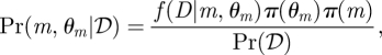
Thus our problem is to identify the model—together with the model parameters—which best explains the data [18]. In a Bayesian framework, we thus seek to determine

2.1

where π(m) and π(θ_m) denote the priors for model m and its associated parameter set θ_m, respectively, and f(D|m, θ_m) is the data-generating process for model m, 1 ≤ m ≤ q; Pr(𝒟) is a normalization constant that is also frequently referred to as the evidence [19]. The posterior Pr(m, θ_m|𝒟) is here taken jointly over the parameter spaces of all the models and the (discrete) model indicator variable. The conceptual equivalence between model selection and parameter inference is one of the most appealing features of the Bayesian approach. Unfortunately, however, analytical expressions of the posterior are generally not available, but a host of computational approaches have been developed that allow the numerical evaluation of posteriors and derived quantities.

Marginalizing over model parameters yields the marginal posterior for model m,

2.2

which assigns a probability to model m to be the model that generated the data 𝒟, conditional on the available data, the set of candidate models, ℳ, and the specified model and parameter priors [19,20]. If for a particular model, we have a marginal posterior close to one, then in this framework we would choose this model. If, however, the posteriors of several models are roughly equally large and no clear best model emerges, then we can (or should) use Bayesian model averaging for any further analysis.

The principal difference between statistical inference and design as discussed here is that, in the former, we have data and seek to reconstruct the model that is most likely to have generated the data [21]; in the latter case, we have an idea of the model/system outputs that we would like to see (such as adapation as in Ma et al. [22] or Barnes et al. [21]). The task then is to learn the structure of the system that is most likely to generate these desired data. As long as we can encode our design objectives in an appropriate way, we can use inferential techniques in the design of synthetic or engineered systems.

We thus replace the observed data 𝒟 by surrogate data, 𝒟_S, that embody our design objectives appropriately, and then determine the marginal posterior probability of each candidate model to deliver these specified outcomes. And just as in the case of the statistical inference, or reverse-engineering, problem, the more detailed 𝒟_S becomes, the more intricate the search for a suitable model gets. This gives rise to the second difference between design and inference: while the choice of a suitable cost-function which rewards models for fit to the data is typically obvious, choosing a cost-function for design may also take into account other factors. In addition to satisfying the design objectives, other factors may also play an important part. In the context of synthetic biological systems, for example, cost and safety considerations may override the ‘fit’ of the model to 𝒟_S. We will return to this point in the penultimate section.

3. Sequential algorithms for inference-based modelling

For simplicity, we will refer to data and design objectives collectively as data and denote these by 𝒟. As mentioned before, analytical expressions for the posterior, equation (2.1), are generally not available. Markov chain Monte Carlo (MCMC) methods have risen to great prominence among the computational tools capable of representing posterior distributions numerically. There is a substantial literature in the area of computational statistics. Here, however, we focus instead on sequential algorithms [23]. While sequential approaches were initially conceived to cope with problems where data are produced in a sequential fashion and inferences were improved as new data became available, sequential Monte Carlo (SMC) and Kalman-filtering-type approaches can also be used on the whole data. Then the sequential algorithms yield increasingly better estimates for the posterior distribution.

Below we will consider highly nonlinear dynamical systems. For these evaluation of the likelihood,

is generally not straightforward [24, 25], and in many cases computationally prohibitive. Here, we develop two complementary frameworks that pursue different strategies in order to study complex dynamical systems.

3.1. Unscented Kalman filter for parameter inference

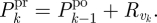
The Kalman filter [26] has been one of the main workhorses for state estimation, but can also be applied for parameter inference, and has been used widely in time-series analysis [27]. We consider the case of estimating the parameters, θ, of a nonlinear mapping g(·) from a sequence of inputs x_ti (which may also be unknown), and noisy observed outputs, 𝒟 = {d₁, … ,d_n}, obtained at times t_i with 1 ≤ i ≤ n. The filter is an example of recursive Bayesian estimation in which at step k, the current estimated parameter distribution conditioned upon data d_j for j < k, is used to make a prediction, , for the next data point. This estimate is then compared with the actual observation, d_k, in order to arrive at updated estimates for θ (and x_k if it is unknown).

The Kalman filter is based on the assumption that dynamics are linear and any noise entering the dynamics and/or the observations is Gaussian-distributed. We are, however, dealing with highly nonlinear problems in both systems and synthetic biology, and non-Gaussian noise. Several extensions to the standard Kalman filter have been proposed, the two most prominent of which follow very different strategies: the extended Kalman filter copes with nonlinearities by Taylor expanding the dynamics to first order [28]. The unscented Kalman filter (UKF) allows for arbitrarily complex dynamics but captures probability distributions to finite order, typically by focusing on mean and variance (i.e. approximating noise by Gaussian noise models) [29–31].

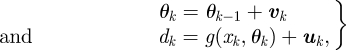
Here, we follow the second approach, and propagate our prior parameter distribution—assumed to be sufficiently well approximated by a Gaussian—through the exact system dynamics. This is achieved by carefully choosing a set of parameters Ξ_k = (χ₀, … ,χ_2L)—where each χ_i is known as a sigma point, and L is the total number of parameters (and states if desired) to be inferred—which completely capture the statistics of the prior distribution. These may be propagated individually through the system and reassembled to approximate the distribution of the output. For the moment, we will consider parameter estimation rather than model selection. We begin by defining the state space model,

3.1

where g(·) is the nonlinear observation function with parameter vector θ_k, u_k ∼ 𝒩(0,R_uk) and v_k ∼ 𝒩(0,R_vk) are the measurement noise and artificial process noise driving the system with covariance matrices R_uk and R_vk, respectively. x₀ are the initial conditions that can also be included into the parameter vector if they are unknown.

We then have for the UKF

• U1 Initialization:

  

  Set k = 1.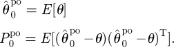
• U2 Prediction: while k ≤ n

  

  and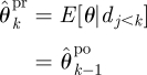

  
• U3 Update:

  
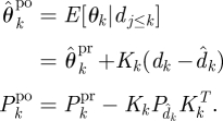  Here, we have

  

  with the sigma point set Ξ_k and weights ω_i given by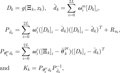

  

  where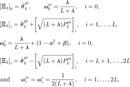

  

  and parameters κ, α and β may be chosen to control the positive definiteness of covariance matrices, spread of the sigma points and error in the kurtosis, respectively.

The 2L + 1 sigma points, Ξ_k (in U3), together with the corresponding weights ω_i^c/m, describe the distribution over the parameter state up to the second moment of the probability distribution. That is, we approximate the probability distribution up to and including the second moment of the distribution; we can go beyond this at increased computational cost. For more complex likelihood surfaces, the UKF therefore gives us a local (Gaussian) look at the posterior. In order to characterize parameter space more globally, multiple runs of the UKF may be used with priors chosen to cover the regions of interest.

Crucially for our purposes, the observation function, g(·), can be arbitrarily complex (subject to the usual regularity conditions) and along with the data, 𝒟—which other than an observed dataset, may also be any function of the data, or even expected or desired qualitative/quantitative characteristics of the system's behaviour [32]—may be chosen to explore various features of interest of the dynamical system. This great, and thus far under-explored, flexibility allows us to use the UKF to determine a set of parameters commensurate with the objectives set out prior to the analysis and encoded in 𝒟. In addition to data and conventional surrogate data (e.g. to condition on design objectives), this may include

•  — stability properties of the stationary state,

•  — existence of bifurcations, and

•  — boundedness of behaviour.

Below we will illustrate this approach in the context of the attractor structure.

The UKF is a natural complement to the approximate Bayesian computation (ABC) approaches discussed below. We are able to tackle larger problems because of the simplified representation of the probability distributions.

3.2. Approximate Bayesian computation

Circumventing explicit evaluation of the likelihood by directly simulating from the data-generating model(s), ABC methods [33–36] are increasingly being applied, especially in inferentially demanding contexts such as evolutionary and systems biology. They work by comparing simulated and observed/desired data and rejecting all parameter/model combinations that fail to provide a satisfactory description of the data. In their simplest form, they work as a simple rejection algorithm.

•  (i) Draw m* from the prior π(m).

•  (ii) Sample θ* from the prior π(θ_m*).

•  (iii) Simulate a candidate dataset D* ∼ f(D| θ*, m*).

•  (iv) Compute the distance. If Δ(𝒟, D*) ≤ ε, accept (m*, θ*), otherwise reject it.

•  (v) Return to (i).

Here, Δ(x,y) can be any suitable distance measure, and ε > 0 is the tolerance level which is set by the user. Once a sample of N particles (parameter vectors) has been accepted, the approximate marginal posterior distribution is given by

Here, we compare the complete data; in principle, we may want to choose to compare summary statistics, which can have advantages for very complicated data structures. But great care has to be invested into the choice of the best summary statistics if we want to perform model selection. This is because choice of insufficient statistics can lead to spurious results for the marginal posterior distribution as discussed by Robert et al. [37].

This simplicity of ABC algorithms is deceptive, as for practical applications, the simple rejection scheme is computationally too inefficient. A range of computational schemes based on MCMC, and especially SMC methods have been proposed and here we follow the algorithm introduced by Toni et al. [35] and Toni & Stumpf [38]:

• A1 Initialize ε₁, … ,ε_T.

  Set the population indicator t = 1.

• A2.0 Set the particle indicator i = 1.

• A2.1 If t = 1 sample (m**, θ**) from the prior distribution Pr₀ (m, θ) = π (m, θ).

  If t > 1 sample m* with probability Pr_t−1(m*) and draw m** ∼ KM_t(m|m*).

  Sample θ* from previous population {θ(m**)_t−1} with weights w_t−1 and draw θ** ∼ KP_t,m**(θ|θ*).

  If π(m**, θ**) = 0, return to A2.1.

  Simulate a candidate dataset D* ∼ f(D|θ**, m**).

  If Δ(𝒟, D*) > ε_t, return to A2.1.

• A2.2 Set (m_t⁽ⁱ⁾, θ_t⁽ⁱ⁾) = (m**, θ**) and calculate the weight of the particle as

  

  where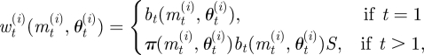

  
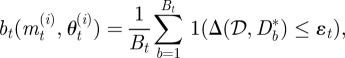  1(Δ(𝒟, D_b^*) ≤ ε_t) denotes the indicator function (=1 if Δ(𝒟, D_b^*) ≤ ε_t and =0 otherwise), and

  

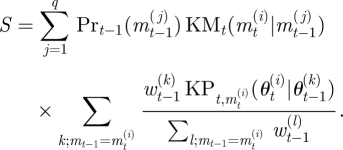
  If i < N set i = i + 1, go to A2.1.

• A3 Normalize the weights w_t.

  Sum the particle weights to obtain marginal model probabilities,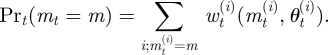

  

  If t < T, set t = t + 1, go to A2.0.

Here, KM and KP are model and parameter perturbation kernels, respectively; B_t ≥ 1 is the number of replicate simulations for a fixed particle.

In practical applications, the choices of ε_t, 1 ≤ t ≤ T, and the perturbation kernels, KM and KP, B_t, can matter a great deal. Obviously, choice of priors will also affect inferences; the distance metric Δ(x,y) should have negligible impact as ε_T → 0. Much of this is still an area of ongoing research, but the package ABC-SysBio [39] offers a convenient implementation of the ABC SMC algorithm and can be used for model selection. The computational power provided by graphics processing units has enabled the application of these methods to problems of increasing complexity [40]. In the following section, we will illustrate the use of this framework in both inference and design settings.

4. Learning the structure of natural systems and successful designs

Here, we illustrate the uses of the ABC SMC and UKF approaches outlined above. We will start with parameter estimation and model selection in the ABC framework. Here, we will stress the conceptual similarities between inference and design.

4.1. Parameter estimation for dynamical systems

The repressilator [41] has become one of the canonical model systems for systems and synthetic biology. It is a simple circuit of three genes and their respective protein products, where protein 1, y₁, inhibits expression of gene 2, x₂; protein 2, y₂, inhibits the expression of gene 3, x₃; and protein 3, y₃, finally, inhibits x₁. In mathematical form, we write for the simplest case of shared kinetic parameters,

4.1

where x_i and y_i denote the mRNA and protein concentrations corresponding to gene i. The index i cycles over the set {1,2,3}. The structure and mathematical details of this model are discussed elsewhere [35].

This model and its generalizations [42] have been studied extensively and it is also included among the examples of the ABC-SysBio package [39], which implements ABC SMC for dynamical systems. In figure 3, we show the resulting posterior probability distributions obtained from simulated data, assuming flat priors for all four parameters. This figure shows the complexity of posterior parameter distributions, even for very small dynamical systems: posterior distributions show considerable levels of correlation and in some directions are still extending over large regions (marginals may even cover the whole prior range).

Figure 3.

Contour plots and marginal densities of the (ABC) posterior distributions for the repressilator model. The distributions are plotted over the prior ranges. The Hill exponent is most reliably inferred, whereas the transcription rate α is least constrained by the (simulated) data. See the examples of the ABC-SysBio package for further details (http://abc-sysbio.sourceforge.net). Also noteworthy is the high level of correlation between n and β.

This is a typical finding for dynamical systems: Sethna and co-workers [43,44], and subsequently other authors [45,46], have found that the likelihood or posterior for the parameters of dynamical systems tend to be flat, even when unrealistically large data were used. Furthermore, correlation between parameters appears to be ubiquitous, which may put practical limits on the use of statistical approaches that assume independence between parameters. This is mainly owing to the fact that dynamical systems tend to be mechanistic and attempt to represent the underlying physical processes. This often means that they contain more parameters and only certain combinations are inferable.

The problem of the complexity of likelihood surfaces or posterior distributions of dynamical systems is further exacerbated by the fact that these also depend subtly on a host of dynamical features of such systems, such as the existence of bifurcations and initial conditions. While posteriors that cover large areas may seem disappointing, more recent studies, albeit confirming such findings, also clearly indicate that parameters which are hard to infer have only negligible impact on the system outputs. On the other hand, all parameters that, when varied slightly, yield very different system outputs, tend to be inferred easily. Following [44] such parameters (or parameter combinations) are referred to as ‘sloppy’ and ‘stiff’, respectively. Many of these problems are most naturally studied using the observed or expected Fisher information [47], also for stochastic dynamical systems [48].

4.2. Qualitative design with the unscented Kalman filter

As we have seen in the previous example, the parameter posterior, Pr(θ|𝒟), for a dynamical system can extend over large areas in parameter space. Reporting such high-dimensional and decidedly non-normal probability distributions generates new challenges but is important given that point estimates carry only limited information. Here, we return to the parameter estimation problem. But rather than looking for quantitative agreement between data and a mathematical model, we seek to determine a set of parameters that gives rise to certain type of qualitative behaviour [32].

One way of specifying or encoding qualitative behaviour of a dynamical system is via its Lyapunov spectrum [49]. For a dynamical system

which is the solution of an ordinary differential equation system

we define the Lyapunov exponents as the rate at which initially arbitrarily close trajectories diverge or converge exponentially with time under the influence of the dynamical system's vector field. More formally, if δy(t) denotes the difference between two trajectories that at time t = 0 were separated by δ₀ > 0, the Lyapunov exponents are the eigenvalues of the matrix Λ defined by

4.2

The leading eigenvalue, λ₁, determines to a large extent the dynamical behaviour of the solution. For λ₁ < 0 all initially nearby solutions will converge and consequently the system will have a single stable equilibrium solution. For λ₁ > 0 trajectories will diverge and the attracting state of the system will depend sensitively on the initial conditions; such dynamical behaviour is commonly referred to as ‘chaotic’. Finally, for λ₁ = 0, trajectories will neither converge nor diverge and the system's attractor will have an oscillatory structure. While Lyapunov exponents are costly to calculate in practice, they do capture the qualitative dynamical behaviour comprehensively and are therefore a useful feature to consider when designing dynamical systems, or specifying their qualitative behaviour.

The UKF now allows us to identify parameter sets that give rise to certain types of dynamical behaviour, if we define the state of the system in terms of the leading Lyapunov exponent (or the entire spectrum) that we desire the system to exhibit. That is, we specify the set of Lyapunov exponents, λ_i, and, starting from an arbitrary starting point, θ₀, we iterate through the UKF procedure until the procedure delivers a set of parameters that are in concordance with the desired system output (characterized by the specified values of λ_i).

In figure 4, we illustrate this in two contexts. First in figure 4a, we infer parameters for the Hénon attractor, one of the canonical models used to study and illustrate the effects of chaotic dynamics for discrete time-dynamical systems.

Figure 4.

The UKF achieves the design objectives in a sequential fashion. In (a), we have given it the task to recreate the Lyapunov spectrum of the classical Hénon map, which is achieved very quickly. In (b), we set it the task of finding an oscillatory solution for the repressilator. We show the convergence of the model parameters to values which meet the design criteria over the required iterations. At the top of both figures, we illustrate some of the attractor structures attained along the way.

H Hénon map:

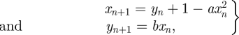4.3

where a and b are free parameters.

Here, we start from a parameter choice for which the system exhibits oscillations and drives it towards values for which we recover the classical attractor structure. In figure 4b, we revisit the repressilator again, given by equations (4.1). Again we start from a random vector which lies in the region where the system's attractor occupies a stable equilibrium point and drives it into an oscillatory regime by specifying λ₁ = 0. For the repressilator, this tends to happen very quickly.

Both examples serve only as illustrations of the use of the UKF and qualitative considerations in the design of dynamical systems. We find that this approach is particularly well suited if the correct qualitative behaviour is paramount. This may, however, also happen in inference: simple optimization approaches can get stuck in regions with the qualitatively wrong behaviour (for example, when a straight line is chosen to approximate an oscillatory solution). By specifying the correct qualitative target behaviour via the (leading) Lyapunov exponent(s), we can guide the solution towards the correct behaviour. This may, for example, aid in eliciting suitable priors for further quantitative inference tasks (e.g. using ABC or exact Bayesian approaches). Overall qualitative inference has received very little attention thus far [50–52], but the combination of suitable statistical tools coupled to appropriate encoding of qualitative features holds a lot of promise both for the inference and the design setting. The types of qualitative behaviour we may want to consider are summarized together with appropriate criteria in table 1.

Table 1.

The ‘zoo’ of possible behaviours relevant for synthetic biology design.

qualitative behaviour	distance/objective functions
stability	Lyapanov exponent λ1 < 0
oscillations	Lyapanov exponent λ1 = 0
	complex eigenvalues of the Jacobian
chaos	Lyapanov exponent λ1 > 0
hyper-chaos	Lyapanov exponents λ1 > 0 and λ2 > 0
switch	zero eigenvalue of the Jacobian
filters	L2 norm between observed and desired frequency response

4.3. Model choice and design using approximate Bayesian computation

In a design setting, we often have a choice of available designs with a wide range of potential parameters which would generate system dynamics that fulfil our specifications. In either case, we can marginalize over the parameter space in order to obtain posterior probabilities,

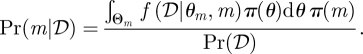4.4

In design applications, 𝒟 can be any set of specified system behaviours. The approach outlined above allows us to compare the probability of different models to achieve the design objectives. Here, a probabilistic approach is beneficial if the system dynamics exhibits elements of intrinsic or extrinsic stochastic behaviour.

4.3.1. Classic oscillators

As a simple illustration, in figure 5 we compare the ability of three dynamical systems to exhibit certain types of oscillatory behaviour. We compare three mathematical models describing biological oscillators, which had been considered previously [53].

Figure 5.

Marginal probabilities for the three classic oscillator models (see main text) to reach the design objectives on (a) frequency and amplitude, and (b) support of a Hopf bifurcation. Model posteriors were obtained using ABC SMC as outlined in the text.

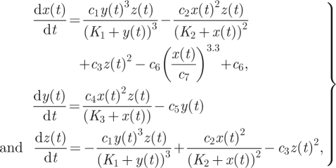
M₁ Meyer–Stryer oscillator:

4.5

where c₄ is free and the other parameters are fixed at c₁ = 6.64, c₂ = 5, c₃ = 0.0000313, c₅ = 2, c₆ = 0.5, c₇ = 0.6, K₁ = 0.1, K₂ = 0.15, K₃ = 1 and the initial conditions are x₀ = 0.1, y₀ = 0.01, z₀ = 25.

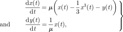
M₂ Van der Pol oscillator:

4.6

where μ is free, x₀ = 0.1 and y₀ = 0.

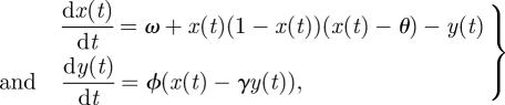
M₃ FitzHugh–Nagumo oscillator:

4.7

where ϕ is free, θ = 0.2, ω = 0.112, γ = 2.5, ν₀ = 0 and w₀ = 0.

All of these systems can exhibit oscillatory behaviour and have been proposed in different contexts as models of real-world biologically oscillating systems.

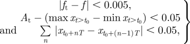
We illustrate the design approach by imposing two different sets of objectives. First, we demand that the oscillations occur at a frequency of 0.02 Hz (within the region 0.0188–0.0298) and that the amplitude of x(t) exceeds 0.1 (figure 5a). This is achieved by simulating systems for t = 200 s and imposing the following design constraints:

4.8

where n is an integer, f_t is the target frequency (=0.02), f is the frequency determined from the largest component of the Fourier spectrum, A_t is the target amplitude (=0.1), T is the target period and t₀ is a cut to remove initial transients (=50 s). These constraints are applied to the first species in all three models although the target species can change the posterior distribution significantly [21]. Second, we require that only the system is able to undergo a Hopf bifurcation [54] (figure 5b); a distance function which allows us to specify this type of behaviour is given by

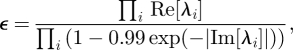4.9

where the λ_i are the eigenvalues of the linearized systems around the steady state [55]. This distance function decreases as the real part of a pair of complex conjugate eigenvalues moves from − inf to 0 giving rise to purely imaginary eigenvalues and limit-cycle oscillations. Here, we used ε = 0.001 as the final threshold.

As we can see in figure 5, the three models show some differences in their respective abilities to produce the desired behaviour. The Van der Pol oscillator, for example, appears less able to deliver the first design objectives than the other two models, which are roughly equally proficient in the first case but start to differ considerably under the second, less-restrictive design objective. Here, we find that the simple FitzHugh–Nagumo oscillator exhibits Hopf bifurcation more reliably than the other two models. In addition to the marginal model probabilities, we also, of course, obtain estimates for the parameter regions that are commensurate with the desired behaviour, which allows us to assess, for example, biophysical constraints that need to be fulfilled by real systems.

Depending on the desired system behaviour, the balance may tip in favour of any of these oscillators. But as we see in figure 5a, sometimes a tie between different models may mean that we have to defer to other factors to choose the best model. In the case of a choice between the Meyer–Stryer and FitzHugh–Nagumo oscillators, for example, we may prefer the simpler model because of the potentially higher ‘cost’ of implementing the three-species model. Including additional factors into the cost function is straightforward in Bayesian decision problems, and is also possible (and desirable) in the design problem as outlined here.

4.3.2. Synthetic in vitro transcriptional oscillators

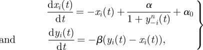
An example of how this approach can be applied to synthetic biological design is demonstrated by considering three in vitro synthetic transcriptional oscillators previously constructed using DNA–RNA circuits [56].

D_I a two-switch negative feedback oscillator:

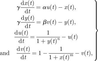4.10

where α, β, γ, n, m, x₀, y₀, u₀ and v₀ are free parameters.

D_II an amplified negative feedback oscillator:

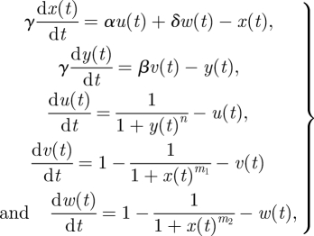4.11

where α, β, γ, δ, n, m₁, m₂, x₀, y₀, u₀, v₀ and w₀ are free parameters.

D_III a three-switch ring oscillator:

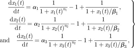4.12

where α_i, β_i, n_i and x_i(0), i ∈ {1,2,3}, are free parameters.

All three systems were constructed with the two-switch negative feedback oscillator demonstrating the most robust oscillations. While the authors eventually used more complex models to achieve agreement with experimental data, these simple models were used to understand the principles of operation.

Our approach in this example was to first use the UKF to determine regions of parameter space giving rise to oscillatory behaviour (λ₁ = 0). The UKF was run 200 times with parameters sampled over the region [0,100] for α, β, γ, [0,25] for m, n and initial conditions sampled over the region [0,5]⁴ using latin hypercube sampling. Examples of the resultant distributions for the two-switch negative feedback oscillator (D_I) are given in figure 6. The ranges from the UKF parameter distributions were then used as priors for an ABC model selection analysis with the Hopf bifurcation criterion (equation (4.9)) as our desired design objective which gives rise to limit-cycle oscillatory solutions (though the upper bound on Hill coefficients was set to 10). Figure 7 illustrates the results of this analysis, which show that the two-switch negative feedback oscillator clearly outperforms the other two for these design objectives. This demonstrates the balance between model complexity (number of parameters) and the achievement of the design objectives which will be discussed below. Figure 8 shows the ABC posterior for the two-switch negative feedback oscillator. The desired behaviour is most sensitive to the Hill coefficients m,n and least sensitive to α.

Figure 6.

UKF parameter distributions for oscillatory behaviour (λ₁ = 0) for the two-switch negative feedback oscillator (D_I). These were generated by running the UKF 200 times with parameters sampled over the region [0,100] for α, β, γ, [0,25] for m, n and initial conditions sampled over the region [0,5]⁴. The exact ranges of the resultant parameter distributions are shown.

Figure 7.

Marginal probabilities for three in vitro synthetic oscillator designs to reach the design objectives of support of a Hopf bifurcation. Model posteriors were obtained using ABC SMC as outlined in the text.

Figure 8.

Contour plots and marginal densities of the (ABC) posterior distributions for the two-switch negative feedback oscillator (D_I). The distributions are plotted over the prior ranges. The desired behaviour is most sensitive to the Hill coefficients m,n and least sensitive to α.

5. Inference and robust behaviour

In the earlier-mentioned examples, the focus has been on evaluating the posterior distributions, Pr(θ|𝒟) or Pr(m,θ_m|𝒟). This incurs considerable computational costs and, given that we have to make some approximations in both approaches presented here, we may want to consider the underlying rationale.

Optimization methods locate the relevant extrema in some objective or cost function. Thus, for a single model they provide us with the parameter value that, for example, maximizes the likelihood of observing the given data. Comparing different models in an optimization framework is not always straightforward as it requires a number of additional heuristics and assumptions; information criteria [57] such as the Akaike information criterion, Bayesian information criterion or deviance information criterion can be used to compare the explanatory power of different models in a way that penalizes against overly complicated models. But such post hoc measures can be problematic, and perhaps more worryingly, optimization-based approaches typically lack appropriate model selection mechanisms entirely.

The advantages of the computationally much more costly inferential frameworks advocated here are easily illustrated in figure 9. We assume that we have data (circles in the inset to the figure) and two competing models for which we have obtained posteriors for the single parameter describing both models. The maximal posterior estimate of the ‘grey’ model is higher than that of the ‘black’ model; simulating from this model for the maximum parameter, , yields a curve (solid grey line) which perfectly fits the data for the grey model. However, perturbing the parameter slightly by a small amount, δ, rapidly deteriorates the fit between model and data (dashed grey line). For the black model, we observe that the maximum a posteriori estimate results in a good but not perfect fit (solid black line); adding a small perturbation to a value results now, however, in a less severely compromised fit (dashed black curve). In evolutionary biology, robustness has sometimes been referred to as ‘survival of the fattest’. Thus, height of the posterior probability curve, or optimality of a cost function in other words, might suggest that the grey model is to be preferred, while robustness to variation in the parameter would tip the balance in favour of the black model. In fact, in a Bayesian framework, the marginal likelihood gives an objective criterion for model selection. This naturally strikes a balance between model performance and robustness (and, of course, model complexity is implicitly dealt with in this framework).

Figure 9.

Illustration of the relative trade-off between model fit and model robustness (see main text for details) in the light of some data 𝒟 = {d₁, … ,d_n}.

6. Discussion

In both inference and design, we seek to balance model fit/performance with robustness. Many engineering approaches have been devised in settings where stochastic effects are ignored, whereas randomness is inherent to the statistical perspective. Hence, some elegant approaches that are applicable in deterministic modelling contexts [58] are not readily applicable to processes where intrinsic or extrinsic noise affects the dynamics and behaviour of a system. In such contexts, we may prefer the computational burden incurred by the approaches described above (linear in the number of parameters for the UKF and approximately exponential for ABC SMC) over the potential pitfalls that optimization methods (e.g. [59,60]) can encounter when confronted with noisy and stochastic dynamics.

From our point of view, the principal difference between inference and design is whether we seek to elucidate the structure that has given rise to some observed data, or the structure that will give rise to the type of output which we would like to observe. This change in perspective allows us to apply the whole apparatus (and, in our view, the inherent advantages) of Bayesian inference to design problems. If we are furthermore, as envisaged in synthetic biology, dealing with libraries of standardized and well-characterized basic parts or components, then we can begin to construct integrated design platforms that explore the available model space (in terms of the available components) and search for solutions that meet the design objectives. Table 1 shows some possible design objectives that can be achieved using our design framework.

Here, a number of challenges need to be faced: unlike electronic systems, biological systems are subject to (specific and unspecific) cross-talk that is mediated by molecules involved in many different processes (e.g. metabolites such as ATP or NADPH); the search space can be vast and efficient heuristics will almost certainly be required to traverse such spaces efficiently; and the correct encoding of design objectives is not always clear a priori. Some of these potential difficulties, of course, mirror many of the problems also encountered in statistical inference and systems biology, or the inverse problem field more generally. The computational approaches developed and illustrated here make best use of the advantages of the Bayesian inferential framework: while we have not focused on this here, they can incorporate prior knowledge and biophysical constraints in their respective prior specifications; they naturally strike a balance between model robustness and performance (or fit to data); and they ensure that parsimony is obeyed as much as possible. In summary, we feel that the Bayesian perspective on design offers a considerate and disciplined way of approaching exciting problems in synthetic biology.

References

- 1.May R. M. 2004. Uses and abuses of mathematics in biology. Science 303, 790–793 10.1126/science.1094442 (doi:10.1126/science.1094442) [DOI] [PubMed] [Google Scholar]
- 2.Nurse P., Hayles J. 2011. The cell in an era of systems biology. Cell 144, 850–854 10.1016/j.cell.2011.02.045 (doi:10.1016/j.cell.2011.02.045) [DOI] [PubMed] [Google Scholar]
- 3.Kwok R. 2010. Five hard truths for synthetic biology. Nature 463, 288–290 10.1038/463288a (doi:10.1038/463288a) [DOI] [PubMed] [Google Scholar]
- 4.Chin J. W. 2006. Programming and engineering biological networks. Curr. Opin. Struct. Biol. 16, 551–556 10.1016/j.sbi.2006.06.011 (doi:10.1016/j.sbi.2006.06.011) [DOI] [PubMed] [Google Scholar]
- 5.Lim W. A. 2010. Designing customized cell signalling circuits. Nat. Rev. Mol. Cell Biol. 11, 393–403 10.1038/nrm2904 (doi:10.1038/nrm2904) [DOI] [PMC free article] [PubMed] [Google Scholar]
- 6.Simons B. D., Clevers H. 2011. Strategies for homeostatic stem cell self-renewal in adult tissues. Cell 145, 851–862 10.1016/j.cell.2011.05.033 (doi:10.1016/j.cell.2011.05.033) [DOI] [PubMed] [Google Scholar]
- 7.Batchelor E., Loewer A., Lahav G. 2009. The ups and downs of p53: understanding protein dynamics in single cells. Nat. Rev. Cancer 9, 371–377 10.1038/nrc2604 (doi:10.1038/nrc2604) [DOI] [PMC free article] [PubMed] [Google Scholar]
- 8.Eldar A., Chary V. K., Xenopoulos P., Fontes M. E., Losón O. C., Dworkin J., Piggot P. J., Elowitz M. B. 2009. Partial penetrance facilitates developmental evolution in bacteria. Nature 460, 510–514 10.1038/nature08150 (doi:10.1038/nature08150) [DOI] [PMC free article] [PubMed] [Google Scholar]
- 9.Werhli A., Grzegorczyk M., Husmeier D. 2006. Comparative evaluation of reverse engineering gene regulatory networks with relevance networks, graphical Gaussian models and Bayesian networks. Bioinformatics 22, 2523–2531 10.1093/bioinformatics/btl391 (doi:10.1093/bioinformatics/btl391) [DOI] [PubMed] [Google Scholar]
- 10.Wang M., Augusto Benedito V., Xuechun Zhao P., Udvardi M. 2010. Inferring large-scale gene regulatory networks using a low-order constraint-based algorithm. Mol. Biosyst. 6, 988–998 10.1039/b917571g (doi:10.1039/b917571g) [DOI] [PubMed] [Google Scholar]
- 11.Pe'er D., Hacohen N. 2011. Principles and strategies for developing network models in cancer. Cell 144, 864–873 10.1016/j.cell.2011.03.001 (doi:10.1016/j.cell.2011.03.001) [DOI] [PMC free article] [PubMed] [Google Scholar]
- 12.Lèbre S., Becq J., Devaux F., Stumpf M. P. H., Lelandais G. 2010. Statistical inference of the time-varying structure of gene-regulation networks. BMC Syst. Biol. 4, 130. 10.1186/1752-0509-4-130 (doi:10.1186/1752-0509-4-130) [DOI] [PMC free article] [PubMed] [Google Scholar]
- 13.Wilkinson D. 2009. Stochastic modelling for quantitative description of heterogeneous biological systems. Nat. Rev. Genet. 10, 122–133 10.1038/nrg2509 (doi:10.1038/nrg2509) [DOI] [PubMed] [Google Scholar]
- 14.Klipp E., Herwig R., Kowald A., Wierling C., Lehrbach H. 2005. Systems biology in practice. Weinheim, Germany: Wiley-VCH; 10.1002/3527603603 (doi:10.1002/3527603603) [DOI] [Google Scholar]
- 15.Wilkinson D. J. 2007. Bayesian methods in bioinformatics and computational systems biology. Brief. Bioinform. 8, 109–116 10.1093/bib/bbm007 (doi:10.1093/bib/bbm007) [DOI] [PubMed] [Google Scholar]
- 16.Kim J., Bates D., Postlethwaite I., Ma L., Iglesias P. 2006. Robustness analysis of biochemical networks. IEE Proc. Syst. Biol. 152, 96–104 10.1049/ip-syb:20050024 (doi:10.1049/ip-syb:20050024) [DOI] [PubMed] [Google Scholar]
- 17.Saltelli A., Ratto M., Andres T., Campolong F. 2008. Global sensitivity analysis: the primer. New York, NY: Wiley [Google Scholar]
- 18.Cox D., Hinkley D. 1974. Theoretical statistics. New York, NY: Chapman & Hall/CRC [Google Scholar]
- 19.Gelman A., Carlin J. B., Stern H., Rubin D. 2003. Bayesian data analysis, 2nd edn. Boca Raton, FL: Chapman & Hall/CRC [Google Scholar]
- 20.Andrieu C., Djurić P., Doucet A. 2001. Model selection by MCMC computation. Signal Process. 81, 19–37 10.1016/S0165-1684(00)00188-2 (doi:10.1016/S0165-1684(00)00188-2) [DOI] [Google Scholar]
- 21.Barnes C., Silk D., Sheng X., Stumpf M. 2011. Bayesian design of synthetic biological systems. Proc. Natl Acad. Sci. USA 108, 8645–8650 10.1073/pnas.1017972108 (doi:10.1073/pnas.1017972108) [DOI] [PMC free article] [PubMed] [Google Scholar]
- 22.Ma W., Trusina A., El-Samad H., Lim W. A., Tang C. 2009. Defining network topologies that can achieve biochemical adaptation. Cell 138, 760–773 10.1016/j.cell.2009.06.013 (doi:10.1016/j.cell.2009.06.013) [DOI] [PMC free article] [PubMed] [Google Scholar]
- 23.Jasra A., Doucet A., Stephens D., Holmes C. 2008. Interacting sequential Monte Carlo samplers for trans-dimensional simulation. Comput. Stat. Data Anal. 52, 1765–1791 10.1016/j.csda.2007.09.009 (doi:10.1016/j.csda.2007.09.009) [DOI] [Google Scholar]
- 24.Kirk P., Toni T., Stumpf M. 2008. Parameter inference for biochemical systems that undergo a Hopf bifurcation. Biophys. J. 95, 540–549 10.1529/biophysj.107.126086 (doi:10.1529/biophysj.107.126086) [DOI] [PMC free article] [PubMed] [Google Scholar]
- 25.Vyshemirsky V., Girolami M. A. 2008. Bayesian ranking of biochemical system models. Bioinformatics 24, 833–839 10.1093/bioinformatics/btm607 (doi:10.1093/bioinformatics/btm607) [DOI] [PubMed] [Google Scholar]
- 26.Kalman R. 1960. A new approach to linear filtering and prediction problems. J. Basic Eng. 82, 35–45 [Google Scholar]
- 27.Simon D. 2006. Optimal state estimation: Kalman, H infinity, and nonlinear approaches. Hoboken, NJ: Wiley-Interscience; 10.1002/0470045345 (doi:10.1002/0470045345) [DOI] [Google Scholar]
- 28.Costa P. 1994. Adaptive model architecture and extended Kalman-Bucy filters. IEEE Trans. Aerosp. Electron. Syst. 30, 525–533 10.1109/7.272275 (doi:10.1109/7.272275) [DOI] [Google Scholar]
- 29.Wan E., van der Merwe R. 2000. The unscented Kalman filter for nonlinear estimation. In IEEE Adaptive Systems for Signal Processing, Communications, and Control Symp., AS-SPCC, pp. 153–158 [Google Scholar]
- 30.Merwe R. V. D. 2004. Sigma-point Kalman filters for probabilistic inference in dynamic state-space models. PhD thesis, Oregon Health and Science University, USA. [Google Scholar]
- 31.Jiang Z., Song Q., He Y., Han J. 2007. A novel adaptive unscented Kalman filter for nonlinear estimation. In 46th IEEE Conf. on Decision and Control, pp. 4293–4298 [Google Scholar]
- 32.Silk D., Kirk P. D. W., Barnes C. P., Toni T., Rose A., Moon S., Dallman M. J., Stumpf M. P. H. 2011. Designing attractive models via automated identification of chaotic and oscillatory regimes. (http://arxiv.org/abs/1108.4746) [DOI] [PMC free article] [PubMed] [Google Scholar]
- 33.Marjoram P., Molitor J., Plagnol V., Tavare S. 2003. Markov chain Monte Carlo without likelihoods. Proc. Natl Acad. Sci. USA 100, 15 324–15 328 10.1073/pnas.0306899100 (doi:10.1073/pnas.0306899100) [DOI] [PMC free article] [PubMed] [Google Scholar]
- 34.Sisson S., Fan Y., Tanaka M. 2007. Sequential Monte Carlo without likelihoods. Proc. Natl Acad Sci. USA 104, 1760–1765 10.1073/pnas.0607208104 (doi:10.1073/pnas.0607208104) [DOI] [PMC free article] [PubMed] [Google Scholar]
- 35.Toni T., Welch D., Strelkowa N., Ipsen A., Stumpf M. P. 2009. Approximate Bayesian computation scheme for parameter inference and model selection in dynamical systems. J. R. Soc. Interface 6, 187–202 10.1098/rsif.2008.0172 (doi:10.1098/rsif.2008.0172) [DOI] [PMC free article] [PubMed] [Google Scholar]
- 36.Marin J.-M., Pudlo P., Robert C. P., Ryder R. 2011. Approximate Bayesian computational methods. (http://arxiv.org/abs/1101.0955v2) [Google Scholar]
- 37.Robert C. P., Cornuet J.-M., Marin J.-M., Pillai N. 2011. Lack of confidence in approximate Bayesian computation model choice. Proc. Natl Acad. Sci. USA 108, 15112–15117 10.1073/pnas.1102900108 (doi:10.1073/pnas.1102900108). [DOI] [PMC free article] [PubMed] [Google Scholar]
- 38.Toni T., Stumpf M. P. H. 2010. Simulation-based model selection for dynamical systems in systems and population biology. Bioinformatics 26, 104–110 10.1093/bioinformatics/btp619 (doi:10.1093/bioinformatics/btp619) [DOI] [PMC free article] [PubMed] [Google Scholar]
- 39.Liepe J., Barnes C., Cule E., Erguler K., Kirk P., Toni T., Stumpf M. P. H. 2010. ABC-SysBio—approximate Bayesian computation in Python with GPU support. Bioinformatics 26, 1797–1799 10.1093/bioinformatics/btq278 (doi:10.1093/bioinformatics/btq278) [DOI] [PMC free article] [PubMed] [Google Scholar]
- 40.Zhou Y., Liepe J., Sheng X., Stumpf M. P. H., Barnes C. 2011. GPU accelerated biochemical network simulation. Bioinformatics 27, 874–876 10.1093/bioinformatics/btr015 (doi:10.1093/bioinformatics/btr015) [DOI] [PMC free article] [PubMed] [Google Scholar]
- 41.Elowitz M. B., Leibler S. 2000. A synthetic oscillatory network of transcriptional regulators. Nature 403, 335–338 10.1038/35002125 (doi:10.1038/35002125) [DOI] [PubMed] [Google Scholar]
- 42.Strelkowa N., Barahona M. 2010. Switchable genetic oscillator operating in quasi-stable mode. J. R. Soc. Interface 7, 1071–1082 10.1098/rsif.2009.0487 (doi:10.1098/rsif.2009.0487) [DOI] [PMC free article] [PubMed] [Google Scholar]
- 43.Brown K. S., Sethna J. P. 2003. Statistical mechanical approaches to models with many poorly known parameters. Phys. Rev. E 68, 021904. 10.1103/PhysRevE.68.021904 (doi:10.1103/PhysRevE.68.021904) [DOI] [PubMed] [Google Scholar]
- 44.Gutenkunst R. N., Waterfall J. J., Casey F. P., Brown K. S., Myers C. R., Sethna J. P. 2007. Universally sloppy parameter sensitivities in systems biology models. PLoS Comput. Biol. 3, e189. 10.1371/journal.pcbi.0030189 (doi:10.1371/journal.pcbi.0030189) [DOI] [PMC free article] [PubMed] [Google Scholar]
- 45.Apgar J. F., Witmer D. K., White F. M., Tidor B. 2010. Sloppy models, parameter uncertainty, and the role of experimental design. Mol. Biosyst. 6, 1890–1900 10.1039/B918098B (doi:10.1039/B918098B) [DOI] [PMC free article] [PubMed] [Google Scholar]
- 46.Erguler K., Stumpf M. P. H. 2011. Practical limits for reverse engineering of dynamical systems: a statistical analysis of sensitivity and parameter inferability in systems biology models. Mol. Biosyst. 7, 1593–1602 10.1039/c0mb00107d (doi:10.1039/c0mb00107d) [DOI] [PubMed] [Google Scholar]
- 47.Secrier M., Toni T., Stumpf M. 2009. The ABC of reverse engineering biological signalling systems. Mol. Biosyst. 5, 1925–1935 10.1039/b908951a (doi:10.1039/b908951a) [DOI] [PubMed] [Google Scholar]
- 48.Komorowski M., Costa M. J., Rand D. A., Stumpf M. P. H. 2011. Sensitivity, robustness, and identifiability in stochastic chemical kinetics models. Proc. Natl Acad. Sci. USA 108, 8645–8650 10.1073/pnas.1015814108 (doi:10.1073/pnas.1015814108) [DOI] [PMC free article] [PubMed] [Google Scholar]
- 49.Castiglione P., Falcioni M., Lesne A., Vulpiani A. 2008. Chaos and coarse graining in statistical mechanics. Cambridge, MA: Cambridge University Press; 10.1017/CBO9780511535291 (doi:10.1017/CBO9780511535291) [DOI] [Google Scholar]
- 50.Drees B. L., Thorsson V., Carter G. W., Rives A. W., Raymond M. Z., Avila-Campillo I., Shannon P., Galitski T. 2005. Derivation of genetic interaction networks from qualitative phenotype data. Genome Biol. 6, R38. 10.1186/gb-2005-6-4-r38 (doi:10.1186/gb-2005-6-4-r38) [DOI] [PMC free article] [PubMed] [Google Scholar]
- 51.Jalan S., Jost J., Atay F. M. 2006. Symbolic synchronization and the detection of global properties of coupled dynamics from local information. Chaos 16, 033124. 10.1063/1.2336415 (doi:10.1063/1.2336415) [DOI] [PubMed] [Google Scholar]
- 52.Toni T., Jovanovic G., Huvet M., Buck M., Stumpf M. P. 2011. From qualitative data to quantitative models: analysis of the phage shock protein response in Escherichia coli. BMC Syst. Biol. 5, 69. 10.1186/1752-0509-5-69 (doi:10.1186/1752-0509-5-69) [DOI] [PMC free article] [PubMed] [Google Scholar]
- 53.Tsai T. Y. C., Choi Y. S., Ma W., Pomerening J. R., Tang C., Ferrell J. E. 2008. Robust, tunable biological oscillations from interlinked positive and negative feedback loops. Science 321, 126–129 10.1126/science.1156951 (doi:10.1126/science.1156951) [DOI] [PMC free article] [PubMed] [Google Scholar]
- 54.Jost J. 2007. Dynamical systems: examples of complex behaviour. Berlin, Germany: Springer [Google Scholar]
- 55.Chickarmane V., Paladugu S. R., Bergmann F., Sauro H. M. 2005. Bifurcation discovery tool. Bioinformatics 21, 3688–3690 10.1093/bioinformatics/bti603 (doi:10.1093/bioinformatics/bti603) [DOI] [PubMed] [Google Scholar]
- 56.Kim J., Winfree E. 2011. Synthetic in vitro transcriptional oscillators. Mol. Syst. Biol. 7, 465. 10.1038/msb.2010.119 (doi:10.1038/msb.2010.119) [DOI] [PMC free article] [PubMed] [Google Scholar]
- 57.Burnham K., Anderson D. 2002. Model selection and multimodel inference: a practical information-theoretic approach. New York, NY: Springer. [Google Scholar]
- 58.Mélykúti B., August E., Papachristodoulou A., El-Samad H. 2010. Discriminating between rival biochemical network models: three approaches to optimal experiment design. BMC Syst. Biol. 4, 38. 10.1186/1752-0509-4-38 (doi:10.1186/1752-0509-4-38) [DOI] [PMC free article] [PubMed] [Google Scholar]
- 59.Mendes P., Kell D. 1998. Non-linear optimization of biochemical pathways: applications to metabolic engineering and parameter estimation. Bioinformatics 14, 869–883 10.1093/bioinformatics/14.10.869 (doi:10.1093/bioinformatics/14.10.869) [DOI] [PubMed] [Google Scholar]
- 60.Nocedal J., Wright S. 2006. Numerical optimization, 2nd edn. New York, NY: Springer [Google Scholar]