How to infer gene networks from expression profiles, revisited

Abstract

Inferring the topology of a gene-regulatory network (GRN) from genome-scale time-series measurements of transcriptional change has proved useful for disentangling complex biological processes. To address the challenges associated with this inference, a number of competing approaches have previously been used, including examples from information theory, Bayesian and dynamic Bayesian networks (DBNs), and ordinary differential equation (ODE) or stochastic differential equation. The performance of these competing approaches have previously been assessed using a variety of in silico and in vivo datasets. Here, we revisit this work by assessing the performance of more recent network inference algorithms, including a novel non-parametric learning approach based upon nonlinear dynamical systems. For larger GRNs, containing hundreds of genes, these non-parametric approaches more accurately infer network structures than do traditional approaches, but at significant computational cost. For smaller systems, DBNs are competitive with the non-parametric approaches with respect to computational time and accuracy, and both of these approaches appear to be more accurate than Granger causality-based methods and those using simple ODEs models.

1. Introduction

The phenotypic expression of a genome, including an organism's response to its external environment, represents an emergent property of a complex, dynamical system with multiple levels of regulation. This regulation includes controls over the transcription of messenger RNA (mRNA) and translation of mRNA into protein via gene-regulatory networks (GRNs). Within a GRN, specific genes encode for transcription factors (TFs); proteins that can bind DNA (either independently or as part of a complex), usually in the upstream regions of target genes (promoter regions), and so regulate their transcription. Since the targets of a TF can include genes encoding for other TFs, as well as those encoding for proteins of other function, interactions arise between transcriptional and translational levels of the system to form a complex network (figure 1). Additional influences may arise in the protein and/or gene space including, for example, post-translational and epigenetic effects, further complicating matters.

Figure 1.

A schematic of a GRN adapted from Brazhnik et al. [1]. The GRN consists of four genes, three of which encode for TFs (genes 1, 3 and 4) and one of which encodes for a protein that catalyses the production of metabolite 2 from metabolite 1. The physical interactions of components at the various levels can be projected into the gene space (dashed lines) to illustrate the complex GRN that we wish to recover.

Identifying the structure of GRNs, particularly, with regards to the targets of TFs, has become a major focus in the systems approach to biology. While the genome-wide targets of a particular TF can be elucidated experimentally using ChIP-chip or ChIP-sequencing (ChIP-seq) [2], generating a ChIP-chip/seq dataset for the many thousands of TFs that may be transcriptionally active in cellular function remains technically and often financially prohibitive. Alternatively, identifying the downstream promoter sequences binding a TF can be achieved using the bacterial one-hybrid system [3] and protein-binding microarrays [4], while TFs that can bind a particular promoter sequence in yeast can be identified via the yeast one-hybrid system [5]. As with ChIP-chip/seq, one-hybrid systems do not currently lend themselves to high throughput experimentation, with the added caveat that binding in vitro or in yeast/bacteria does not necessarily imply that the TF can or does bind in its native environment or under particular experimental conditions.

As an alternative (or complementary) approach to the experimental identification of TF targets, measuring the dynamic response of transcription and/or translation can provide useful information about the underlying GRN on a more global scale, provided there is a way to infer the topology of the network (often referred to as ‘reverse-engineering’ in the literature). While measuring the level of protein present in biological systems remains difficult to do on a large scale, measuring the relative abundance of mRNA is comparatively straightforward. Consequently, the generation of highly resolved time-series measurement of transcript levels via multiple microarray experiments has become an increasingly powerful tool for investigating complex biological processes, including developmental programmes [6] and response to abiotic or biotic stress. The inference of GRNs from such time course data has proven useful for disentangling (suspected causal) relationships between genes [7,8], identifying network components important to the biological response, including highly connected genes (so-called ‘hubs’) and capturing the behaviour of the system under novel perturbations [9,10].

To address the various challenges associated with inferring GRNs from transcriptional time series, a number of theoretical approaches have been applied, including ordinary and stochastic differential equations (ODEs/SDEs) [10–12], Bayesian and dynamic Bayesian networks (BNs/DBNs) [7,8,11–13] and information theoretic or correlation-based methods [11,14]. While the relative merits of these competing approaches have previously been discussed in the context of in silico [11,13,15,16] and in vivo networks [8,12,13,15], there remains disagreement as to the best approach. Previous work by Bansal et al. [11], published in 2007, suggests that while ‘further improvements are needed’, network inference algorithms have become ‘practically useful’. Here, we revisit the work of Bansal et al. [11] by assessing the performance of more recent examples of network inference algorithms, using a range of in silico and in vivo datasets.

2. Inference of gene-regulatory networks from time course data

Inference of GRNs from transcriptomic datasets is a notoriously difficult task, primarily because the number of probes (genes) on modern microarrays can be several orders of magnitude greater than the number of independent measurements, even for highly resolved and replicated time course studies [6]. The sheer number of genes, combined with the observation that a significant proportion of expression profiles can be correlated over time [6], means that inferring GRNs from microarray data alone may be inherently unidentifiable. To overcome this problem, the number of genes to be modelled is often artificially reduced by removing flat or uninteresting profiles [6] or by clustering together groups of genes that might be co-expressed [17,18]. Alternatively, when investigating an organism's response to a particular stimulus, in which time series are measured under both control and perturbed conditions, the number of genes can be reduced by including only those that are differentially expressed, i.e. whose expression profiles are different in the control and perturbed datasets [19]. Removing genes in this way can greatly limit the number to be modelled, yielding figures in the range of hundreds to tens of thousands. In most cases, this number is still prohibitively large, requiring prior knowledge or heuristic approaches to reduce the pool further. Problems may nevertheless arise when artificially reducing the number of genes in this manner, for example, by erroneously labelling a particular gene as not differentially expressed. Additionally, even modern microarrays may be missing probes for important genes. In these cases, the absence of an otherwise important gene could have a negative impact on the accuracy of the reconstructed network.

Other notable sources of error in the reconstruction of networks arise when inferring networks from transcriptional data alone. Such models tend to assume protein behaviour to be correlated with transcription, which often appears not to be the case [20], owing to a variety of effects including protein degradation and post-translational modifications.

In subsequent sections, we briefly outline a variety of approaches used to infer networks from time course data, including ODEs, BN and DBNs, non-parametric approaches using Bayesian learning of nonlinear dynamical systems (NDSs), and approaches based upon statistical-hypothesis tests (e.g. t-tests), such as Granger causality.

2.1. Ordinary differential equations

Within the context of GRNs, a coupled set of ODEs represents a deterministic model relating the instantaneous change in mRNA concentration of a gene to the mRNA concentration of all other genes in the system:

2.1

where X_i = {x₁, … , x_M} denotes the vector of mRNA concentrations of the ith gene (of N) at times {t₁, … , t_M}, with time-derivative Ẋ_i = {dx₁/dt, … , dx_M/dt}, Y represents additional time course variables including, for example, protein and metabolite concentrations or other external perturbations, and f(·) represents an appropriate function capturing the relationship between all variables and their instantaneous change, with Θ the vector of model parameters.

In the simplest ODE models, the rate of change in transcription depends on all other transcripts via:

2.2

where a_ij represents a real-valued parameter capturing the influence of gene j upon gene i, with positive values indicating genes that promote transcription of i, negative values indicating repressors of i and zero-entries representing non-parents. In these cases, inference of network structure requires inference of the parameters, a_ij, from time-series data, potentially to be accompanied by post-inference processing to ensure a_ij is sparse. Notable extensions to this basic model include additional terms representing, for example, effects arising from degradation of the mRNA or protein [21], or the influence of external perturbations including drug concentrations [22,23], which may additionally be estimated from the data, or fixed using prior knowledge or experimentation.

When the network structure is known a priori, the functional form of f(·) can instead be chosen to reflect more realistically the underlying assumptions about the nature of GRNs by including, e.g. transcriptional delays and rate-limiting effects designed to mimic the chemical nature of interactions using Michaelis–Menten or Hill-type kinetics. In these models, time-series data might be used to infer a subset of the physically meaningful parameters such as transcription and translation rates and protein-binding rates and affinities. The number of parameters in these physically motivated ODE systems can be significantly large and solutions can be unidentifiable. In these cases, a small subset of parameters might need to be estimated, requiring time-series data from single cells. Additionally, the computational cost of solving such systems of equations can be large, and while non-parametric methods can be employed to speed up inference of parameters [24], these types of ODE systems are more suited to small, well-characterized systems, such as the Arabidopsis clock [25–27] or the NF-κB-signalling pathway [28,29]. However, the realistic nature of such models allow the user to make predictions about the behaviour of the system under new perturbations [10], an approach that has previously been fruitful in identifying novel components of the system [25].

2.2. Bayesian and dynamic Bayesian networks

BNs are directed acyclic graphs (DAGs) in which individual nodes represent random variables, with directed connections (edges) between nodes representing probabilistic conditional independencies. For a GRN, BNs are used to relate the mRNA expression of a gene to the mRNA expression of other genes. Since the network structure of a BN is a DAG, the joint probability density that a network generated the observations, , may be factorized into a product of conditional distributions:

2.3

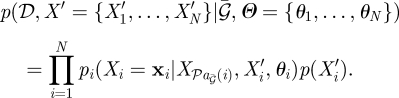
where denotes the parental set of node i, the mRNA/protein/metabolite concentrations of that parental set and Θ represents the free parameters of the probability density function p_i(·). A key limitation of assuming a DAG is the inability to describe feedback loops, an important constituent of GRNs [30,31]. The importance of this is illustrated in figure 2, in which the GRN represented in figure 2a,b may only be represented in terms of a BN as indicated in figure 2c. To overcome these limitations, DBNs were suggested as a model of time course observations [32,33]. For a DBN, an individual gene is no longer represented by a single node but by a series of nodes by unfolding the DAG over time (figure 2d). In the simplest implementation of a DBN the observation at time t_i depends only upon observations at time t_i−1 and equation (2.3) becomes:

2.4

where may now include cyclic structures, N represents the number of genes and M the number of time points in the time series.

Figure 2.

(a) An example system composed of three genes that each encode for a TF that regulates two other genes. The GRN to be recovered from time-series data is projected into the gene space as dashed lines. The time-series observations represent the mRNA levels of genes 1, 2 and 3 as X₁, X₂ and X₃, respectively. (b) A graphical representation of the GRN we wish to recover. (c) BNs cannot represent feedback loops, including self-regulation. Consequently, a BN can, at best, only infer one of three linear pathways. (d) A DBN can be unfolded in time to capture the essence of the GRN, including auto-regulation and feedback loops. (e) In some cases, where observations are missing (in this case observation of gene 1) state-space models may be used to capture the influence of the latent profile.

2.2.1. Missing parameters and variables

A key advantage of BNs and DBNs is the ability to incorporate missing values, including missing time-point observations and missing variables. The influence of a missing variable, such as an unmeasured TF, may be incorporated into a BN by noting the joint distribution is defined as:

2.5

The influence of the missing variable X′ may either be integrated out (marginalized), or inferred as part of the algorithm (figure 2e). A notable example of a DBN that infers missing variables is the Bayesian state-space model (SSM) of Beal et al. [7], which uses a variational approach to infer the hidden states and free parameters of an SSM.

2.2.2. Inference in Bayesian networks and dynamic Bayesian networks and prior knowledge

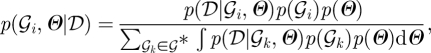
Reverse-engineering of a GRN using a BN or DBN typically involves inferring the graph structure, , the free parameters of the probability density functions, Θ or a combination of both. In theory, the joint probability of a particular network structure, , and model parameters, Θ, may be calculated via Bayes' rule:

2.6

where denotes the set of all allowable graph structures, p(Θ) represents the prior density of Θ and the prior probability of . Enumerating all possible combinations of network structures is often computationally unfeasible while exact marginalization of free-parameters can be analytically intractable. Rather than performing an exact calculation of equation (2.6), quite often approximations are employed, including maximum-likelihood and maximum a posteriori (MAP) approaches, approximations via expectation-maximization (EM) or sampling via Monte Carlo techniques (for a concise introduction to these methods see e.g. [34]).

A key feature of the Bayesian approach is the ability to incorporate prior information. Within equation (2.6), prior information about known connections in a GRN is encoded using the term .

2.3. Non-parametric approaches to nonlinear dynamical systems

In recent years, a novel class of non-parametric algorithms have been suggested which combines the flexibility and advantages of Bayesian learning with NDS [15,35]. A common class of NDS evolves in continuous time as:

2.7

where f(·) denotes an unknown, nonlinear function. Rather than explicitly trying to choose a parametrized form for f(·), as would be the case in an system of ODEs, an alternative strategy is to use a non-parametric approach to capture the effect of the function directly from the data. When the parents of a particular gene, , are known a priori, the task becomes one of identifying the potentially nonlinear relationship between a series of outputs, , from a series of inputs , which may be achieved by assigning the function f(·) a Gaussian process prior [36]. The conditional probability density of the observation, , is then defined by a multivariate normal distribution:

2.8

where μ represents the process mean and K the covariance. A probability distribution over possible parental sets for the ith gene can then be calculated via Bayes' rule as:

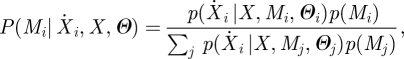2.9

where M_j represents the jth possible parental set of gene i and Θ_j represents the hyperparameters of the Gaussian process. This calculation requires a separate Gaussian process model of the dynamics for each possible set of parents, which scales super-exponentially with the number of TFs. By limiting the maximum in-degree for each node, i.e. limiting maximum number of parents, this scaling becomes polynomial [15,35], and the denominator in equation (2.9) may be feasibly calculated. Equation (2.9) may be applied node-by-node to all possible genes in a system, to evaluate the distribution over network structures.

The behaviour of each of the separate Gaussian process models depend upon the choice of hyperparameters Θ. Although it would be preferable to integrate out these hyperparameters, the solution is not analytically tractable and would require sampling-based approaches. Aïjö & Lähdesmäki [15] instead infer a separate set of hyperparameters for each of models in the denominator by maximizing the marginal likelihood:

2.10

Alternatively, studies by Klemm [35] suggest using a common hyperparameter for all models in the denominator of equation (2.9), which can be inferred along with the distribution over parental sets using an EM approach.

2.3.1. Derivative estimation for continuous time systems

Microarray time course datasets measure the mRNA expression profiles, X_i, and consequently, the time-derivative must first be estimated from the data in order to apply the continuous non-parametric models outlined in §2.3. Studies by Aïjö & Lähdesmäki [15] suggest using a discrete approximation:

2.11

Alternatively, by assuming the mRNA expression profile of the ith gene corresponds to a Gaussian process (e.g. [19]), and noting that the derivative of a Gaussian process is itself a Gaussian process [24,36,37], Klemm [35] suggest that the derivative can be approximated as:

2.12

where Θ is taken to be the MAP estimator, and μ and K represent the mean and covariance, respectively.

2.3.2. Discrete time nonlinear dynamical systems

A second class of NDSs outlined in Klemm [35] evolves over discrete time as:

2.13

where, again, f(·) represents an appropriate nonlinear function. Where the parental set is known, learning this function essentially involves learning a relationship between a vector of observations X_i = {X_i(t₂),X_i(t₃), … , X_i(t_M)}, and the matrix of observations composed of the expression levels of the parental set at the preceding time points, which may again be achieved by assigning the function a Gaussian process prior. As with the continuous time NDS, a distribution over the parental sets may be calculated via Bayes' rule (see equation (2.9)).

2.4. Granger causality

The notion of Granger causality was first introduced within the context of auto-regression models [38]. Informally, a random variable X₁ is said to Granger cause a second variable, X₂, if knowledge of the past behaviour of X₁ improves prediction of X₂ compared with knowing the past of X₂ alone. Typically, this involves calculating the predictive error of X₂ with and without the variable X₁ and performing a suitable statistical test to determine whether or not the more complex model (with X₁) has better explanatory power versus the simpler case. Granger causality can readily be extended to cases of multivariate datasets (e.g. [39]), allowing their use in GRN inference [13].

2.5. Implemented algorithms

In order to evaluate the performance of simple ODEs on time-series data, we use the time-series network identification (TSNI) algorithm of Bansal et al. [23], while Granger causality analysis is implemented using the Granger Causal Connectivity Analysis (GCCA) toolbox [39]. An example of a linear DBN using first-order conditional dependencies can be found in the G1DBN package [40], while a DBN with hidden states is investigated using the variational Bayesian SSM (VBSSM) of Beal et al. [7]. An example of inference using non-parametric NDS can be found in the Matlab package GP4GRN [15]. Additionally, we implement a Matlab version of the algorithms proposed in Klemm [35], which includes an EM implementation of a Gaussian process model for NDS evolving over continuous time (causal structure identification (CSI)^c, §2.3), and one evolving over discrete time (CSI^d, §2.3.2).

3. Network evaluation

Establishing the accuracy of an inferred GRN requires knowledge of a ground-truth (or gold standard) network, against which the inferred network can be ‘benchmarked’. Benchmarking involves counting the number of links correctly predicted by the algorithm (true positives, TP), the number of incorrectly predicted links (false positives, FP), the number of true links missed in the inferred network (false negatives, FN) and the number of correctly identified non-links (true negatives, TN), as illustrated in figure 3. Performance of the algorithm can then be summarized by calculating the true positive rate (TPR, TPR = TP/TP + FN) also known as recall, the false positive rate (FPR = FP/FP + TN), and the positive predictive value (PPV = TP/TP + FP) also known as the precision.

Figure 3.

Illustration of benchmarking recovered GRNs against a known gold standard network. (a) The true gold standard network consists of four genes with three edges, in which genes 1 and 2 both regulate gene 3, which in turn regulates gene 4. (b) The network recovered by inferring the network from time-series data suggests a four gene network in which gene 2 regulates gene 3, with genes 1 and 3 both regulating gene 4. (c) The number of TPs, TNs, FPs or FNs are counted. In this case, the recovered network contains two TPs, one FP, one FN and 12 TNs.

In most cases, however, inference does not identify a single network, but a fully connected network with edges weighted according to, for example, the strength or probability of that particular interaction (compare figure 4b with figure 4a), which may interpreted in terms of a ranked list of connections. A sparser network can be extracted from the list by removing all links with strength or probability below a certain threshold (figure 4c), counting the number of TP, FP, TN and FN and evaluating the TPR/FPR/PPV. By evaluating the performance of the algorithm over a range of such thresholds, the performance can be summarized by: (i) the receiver operating characteristic (ROC) curve, which plots the 1-FPR (equivalent to the specificity) versus the TPR for all thresholds; (ii) the precision-recall (PR) curve, which plots the TPR against the PPV for all thresholds. In all subsequent benchmarking, we evaluate both the ROC and PR curves.

Figure 4.

(a) An example ‘gold standard’ network which consists of four genes with five edges. Gene 1 regulates genes 2 and 3, gene 2 regulates genes 3 and 4 and gene 4 regulates gene 1. (b) The inferred network is a fully connected graph in which particular edges are ranked according to, e.g. the strength or probability of connection. (c) A sparse network can be generated from the fully connected network by removing all edges below a certain threshold. In this example, removing edges below a threshold of 0.1 removes six connections, while a threshold of 0.5 removes nine connections. For threshold the number of TPs, FPs, TNs and FNs can be calculated as in figure 3. A summary of the performance can be obtained using either: (i) the receiver operating characteristic (ROC) curve, which plots 1-FPR versus TPR for all thresholds; or (ii) the precision-recall curve, which plots the TPR versus PPV.

4. Results

4.1. In silico networks

While the targets of TFs may be experimentally identified using a variety of experimental techniques including ChIP-chip/seq [2] and one-hybrid systems [3,5], allowing the validity of individual connections to be verified, establishing a complete gold-standard GRN in biological systems remains technically and financially difficult. This has lead to the emergence of a diverse range of in silico networks from which observations can be generated for benchmarking purposes. Foremost among the in silico networks are those released as part of the dialogue on reverse engineering assessment and methods (DREAM, see also the DREAM homepage¹) [16,10].

4.1.1. DREAM4 10-gene networks

As an example of a small in silico network we make use of the 10-gene networks released as part of the DREAM4 challenge [16,41,42], available for download at the DREAM project homepage. The datasets consist of five separate networks, whose topologies were extracted from known GRNs in Escherichia coli and Saccharomyces cerevisiae. Time-series observations were generated using parametrized SDEs, with observations uniformly sampled (21 time points, single replicate) under five different perturbations, for a total of 105 observations per gene. The datasets include additive measurement noise, modelled upon existing microarray noise.

Depending upon the capability of the algorithms, networks were inferred using either a complete dataset (all five perturbations simultaneously), or a separate network was inferred for each perturbation, with a consensus network evaluated as the average of the five inferred networks. Self-interactions were removed from all networks and performance evaluated by calculating the area under the ROC curve (AUROC) and area under the PR curve (AUPR). For comparison, we evaluated the average AUROC and AUPR scores obtained from 1000 randomly generated adjacency matrices (again removing self-interactions), which yielded scores of approximately AUROC = 0.55 and AUPPR = 0.16–0.19. Additional networks were inferred from steady-state measurements following systematic knockouts or knockdowns of each of the 10 genes using pipeline 1 of Greenfield et al. [10], which yielded AUROC scores of between 0.73–0.9 and AUPR scores in the range 0.27–0.78.

The performance of each of the methods used is summarized in table 1. In general, all methods appeared to perform better than random, with DBNs, non-parametric NDSs approaches, and networks recovered from steady-state data each performing best in at least one of the five datasets.

Table 1.

Average area under the receiver operating characteristic curve (AUROC) and area under the precision-recall (AUPR) curve (in brackets) for each of the 10-gene DREAM4 networks using various inference algorithms. The best overall performance for each network in terms of AUROC/AUPR is indicated in italics, while the best time-series approach (non-steady state) is shown in bold. Bold italics indicates that the best overall performance was a time-series method. CSI^c evolves over continuous time. CSI^d evolves over discrete time.

method	algorithm	network 1	network 2	network 3	network 4	network 5
steady state	knockout	0.90 (0.78)	0.73 (0.27)	0.91 (0.63)	0.84 (0.66)	0.75 (0.37)
	knockdown	0.71 (0.34)	0.62 (0.25)	0.74 (0.46)	0.64 (0.30)	0.68 (0.23)
DBN	G1DBN	0.73 (0.37)	0.64 (0.34)	0.68 (0.45)	0.85 (0.69)	0.92 (0.77)
	VBSSM	0.73 (0.38)	0.66 (0.41)	0.77 (0.49)	0.80 (0.46)	0.84 (0.64)
ODE	TSNI	0.62 (0.27)	0.63 (0.32)	0.58 (0.21)	0.63 (0.23)	0.68 (0.25)
NDS	GP4GRN	0.66 (0.42)	0.69 (0.44)	0.70 (0.47)	0.62 (0.35)	0.86 (0.65)
	CSId	0.72 (0.64)	0.75 (0.54)	0.67 (0.45)	0.83 (0.67)	0.90 (0.78)
	CSIc	0.78 (0.42)	0.73 (0.40)	0.66 (0.29)	0.64 (0.26)	0.75 (0.27)
GC	GCCA	0.67 (0.30)	0.70 (0.47)	0.62 (0.26)	0.80 (0.56)	0.80 (0.58)
random	random	0.55 (0.18)	0.55 (0.19)	0.55 (0.17)	0.57 (0.17)	0.56 (0.16)

DBNs were significantly better than random on all five datasets, with DBNs that incorporate hidden-states (VBSSM) outperforming those that do not (G1DBN) in datasets 2 and 3, while G1DBN performed better on datasets 4 and 5. The two methods performed similarly on dataset 1. In contrast to previous studies of Cantone et al. [12], DBNs were here found to consistently outperform simple ODE-based approaches (TSNI). DBNs also possessed better AUROC/AUPR scores in general than those following reconstruction using Granger causality (GCCA; four out of five datasets), consistent with previous observations that DBNs were better than GC when the number of observations was low [13].

The non-parametric NDSs approaches were consistently found to perform better than random, and were the top-ranked time-series approach in three out of five of the datasets. Interestingly, the EM algorithm of Klemm [35], which used a Gaussian process to estimate the time-derivative and jointly constrained the hyperparameters, performed better than the maximum-likelihood-based approach of Aïjö & Lähdesmäki [15], which used a discrete approximation to the gradient, in three of five of the datasets. The discrete NDS proposed in Klemm [35] performed better than both approaches on four of the datasets. In general, however, the non-parametric NDSs methods did not greatly outperform other, linear methods such as the dynamical BNs.

4.1.2. DREAM4 100-gene networks

As an example of a larger in silico network, we make use of the 100-gene systems of the DREAM4 challenge [16,41,42]. The datasets again consist of five networks whose topology is taken from E. coli or S. cerevisiae networks. Time series consist of uniformly sampled measurements (21 time points, single replicate) simulated using a parametrized set of SDEs under 10 different perturbations. Additive noise modelled upon microarray noise was included.

Recovered networks were inferred as for the 10-gene networks, again removing all self-interactions. For comparison purposes, 100 random networks were generated yielding scores of approximately AUROC = 0.50 and AUROC = 0.002. Additional networks were again inferred from steady-state measurements following systematic knockouts or knockdowns of each of the 100 genes using pipeline 1 of Greenfield et al. [10], which yielded AUROC scores of between 0.74 and 0.88 and AUPR scores in the range 0.15–0.46. Performance of the individual approaches are summarized in table 2.

Table 2.

Average area under the receiver operating characteristic curve (AUROC) and area under the precision-recall (AUPR) curve (in brackets) for each of the 100-gene DREAM4 networks using various inference algorithms. The best overall performance for each network in terms of the AUROC/AUPR is indicated in italics, while the best time-series approach (non-steady state) is shown in bold. Bold italics indicates that the best overall performance was by a time series method. CSI^c evolves over continuous time. CSI^d evolves over discrete time.

method	algorithm	network 1	network 2	network 3	network 4	network 5
steady state	knockout	0.88 (0.46)	0.76 (0.33)	0.80 (0.33)	0.82 (0.33)	0.74 (0.15)
	knockdown	0.68 (0.06)	0.61 (0.02)	0.63 (0.01)	0.66 (0.06)	0.62 (0.02)
DBN	G1DBN	0.68 (0.11)	0.64 (0.10)	0.68 (0.13)	0.66 (0.10)	0.72 (0.11)
	VBSSMa	0.59 (0.08)	0.56 (0.05)	0.59 (0.11)	0.67 (0.10)	0.71 (0.09)
	VBSSMb	0.56 (0.09)	0.57 (0.06)	0.62 (0.12)	0.64 (0.12)	0.70 (0.09)
ODE	TSNI	0.55 (0.02)	0.55 (0.03)	0.60 (0.03)	0.54 (0.02)	0.59 (0.03)
NDS	GP4GRN	0.72 (0.22)	0.62 (0.10)	0.70 (0.16)	0.70 (0.21)	0.69 (0.12)
	CSId	0.71 (0.25)	0.67 (0.17)	0.71 (0.25)	0.74 (0.24)	0.73 (0.26)
	CSIc	0.65 (0.13)	0.56 (0.03)	0.63 (0.07)	0.61 (0.07)	0.60 (0.05)
GC	GCCA	0.60 (0.04)	0.57 (0.04)	0.60 (0.07)	0.58 (0.07)	0.57 (0.03)
random	random	0.50 (0.002)	0.50 (0.002)	0.50 (0.002)	0.50 (0.002)	0.50 (0.002)

^aA single hidden-state.

^bThe hidden state dimension is selected to maximize the marginal likelihood.

The non-parametric NDS algorithms performed best of all the time course methods, with scores significantly greater than other approaches, including DBNs. The performance of the discrete CSI algorithm (CSI^d) was superior to a previous parametrized ODE model, which had been one of the top contenders in the previous DREAM3 network inference challenge, and had AUPR scores of (approx.) 0.23, 0.11, 0.21, 0.19 and 0.14, respectively, in the five DREAM4 100-gene datasets (see fig. 2 of Greenfield et al. [10]). In general, the discrete CSI algorithm (CSI^d) [35] was found to outperform the continuous CSI algorithm (CSI^c) [35] and the related maximum-likelihood approach of Aïjö & Lähdesmäki [15] (GP4GRN). While DBNs did not perform as well as the non-parametric approaches, they did perform better than methods based upon Granger causality and simple ODE systems (TSNI). The latter has previously been acknowledged to perform poorly on larger datasets [23,11], and is not strictly designed for inferring networks but rather the targets of perturbations. Interestingly, while methods using time-series data did not outcompete reconstruction using systematic knockout, non-parametric and Bayesian methods were competitive with networks reconstructed following systematic knockdowns.

Network inference using systematic knockouts was superior to all methods using time-series data tested here. Indeed, networks constructed solely from the knockout data produced the most accurate network topologies in the original DREAM4 challenge. Previous studies have suggested that combining predictions from different inference methods can result in a better, or at least more robust, performance compared with the individual methods alone [42]. In the DREAM4 challenge, a simple combination of time course and knockout data was achieved by the ranking of connections identified from the two datasets and calculating an averaged rank (see pipeline 3 in Greenfield et al. [10]), but this did not appear to perform better than the networks produced from systematic knockouts alone. Subsequent analysis by Greenfield et al. [10] did, however, demonstrate that the two datasets could be used together in a mutually beneficial way. In table 3, we demonstrate the effect of combining time-series data with knockout data for each of the network inference algorithms previously described, using pipeline 3 approach of Greenfield et al. [10]. For the DBNs, the combination of time series with knockout data outperformed reconstruction using knockout data alone in one out of five cases. Simple ODE and Granger causality-based methods using time-series data did not appear to add anything to the knockout data. Conversely, for the NDSs-based approaches the performance using both datasets appears to be better than the knockout dataset alone in two of five cases, and comparable in a third, suggesting that more recent methods can be advantageously combined with knockout data. Producing a knockout for each gene in the network is, however, unrealistic in practice for many organisms, requiring additional biological experiments and explicit knowledge of the genes involved in the network prior to inference.

Table 3.

Average area under the receiver operating characteristic curve (AUROC) and area under the precision-recall (AUPR) curve (in brackets) for each of the 100-gene DREAM4 networks using various inference algorithms combined with the knockout data. The best overall performance for each network in terms of the AUROC/AUPR is indicated in italics, while the best time-series approach (non-steady state) is shown in bold. Bold italics indicates that the best overall performance was by a time series method. CSI^c evolves over continuous time. CSI^d evolves over discrete time.

method	algorithm	network 1	network 2	network 3	network 4	network 5
steady state	knockout alone	0.88 (0.46)	0.76 (0.33)	0.80 (0.33)	0.82 (0.33)	0.74 (0.15)
	knockdown + KO	0.83 (0.39)	0.72 (0.18)	0.76 (0.15)	0.78 (0.22)	0.71 (0.10)
DBN	G1DBN + KO	0.84 (0.31)	0.75 (0.24)	0.79 (0.26)	0.80 (0.26)	0.79 (0.19)
	VBSSMa + KO	0.80 (0.20)	0.70 (0.15)	0.75 (0.15)	0.80 (0.28)	0.79 (0.19)
	VBSSMb + KO	0.78 (0.18)	0.71 (0.16)	0.75 (0.14)	0.78 (0.26)	0.77 (0.17)
ODE	TSNI + KO	0.80 (0.16)	0.71 (0.11)	0.75 (0.13)	0.75 (0.14)	0.75 (0.08)
NDS	GP4GRN + KO	0.84 (0.37)	0.73 (0.24)	0.79 (0.29)	0.80 (0.32)	0.76 (0.22)
	CSId + KO	0.84 (0.38)	0.76 (0.29)	0.80 (0.33)	0.83 (0.38)	0.78 (0.27)
	CSIc + KO	0.81 (0.30)	0.71 (0.11)	0.77 (0.16)	0.77 (0.18)	0.71 (0.12)
GC	GCCA + KO	0.80 (0.20)	0.71 (0.17)	0.76 (0.15)	0.76 (0.12)	0.70 (0.09)

^aA single hidden-state.

^bThe hidden state dimension is selected to maximize the marginal likelihood.

4.2. Synthetic and in vivo networks

While in silico datasets readily allow benchmarking of algorithms on arbitrarily large systems, Werhli et al. [8] note that the data used in such benchmarking represent a simplification of biological systems, suggesting that conclusions based solely upon in silico benchmarking might lead to biased evaluations. While the topology of large-scale, gold-standard biological networks remain unknown, advances in experimental techniques including ChIP-chip/seq and the one-hybrid systems mean that the small-scale biological networks, including the Arabidopsis clock, are now well characterized [25,27]. Similarly, advances in synthetic biology have allowed small networks to been constructed in vivo [12], providing opportunities for testing of algorithms in real biological systems.

4.2.1. In-vivo reverse-engineering and modelling assessment yeast network

A synthetic GRN has previously been constructed in the budding yeast S. cerevisiae [12]. This in-vivo reverse-engineering and modelling assessment (IRMA) network consists of five genes, each of which regulate at least one other gene in the network, and whose expression is negligibly influenced by endogenous genes. Expression within the network is activated in the presence of galactose and inhibited in the presence of glucose, allowing two time course datasets to be generated by Cantone et al. [12]. In the first of these cells were grown in a glucose medium and switched to galactose (switch on) with gene expression monitored over 16 time points using quantitative RT-PCR. In the second dataset, cells were grown in a galactose medium and switched to glucose (switch off) with expression monitored over 21 time points.

The performance of each of the inference algorithms was evaluated in terms of AUROC and AUPR using both the switch on and switch off datasets, again removing self-interactions. For comparison purposes, the performance of randomly generated networks, and networks reconstructed from the steady-state data following systematic knockouts are also included. A summary of performance in terms of AUROC and AUPR can be seen in table 4, with networks inferred from the switch off dataset depicted in figure 5.

Table 4.

Average area under the receiver operating characteristic curve (AUROC) and area under the precision-recall (AUPR) curve (in brackets) for switch on and switch off yeast networks using various inference algorithms. The best overall performance for each network is indicated in italics, while the best time-series approach is shown in bold. Bold italics indicates that the best overall performance was by a time series method. CSI^c evolves over continuous time. CSI^d evolves over discrete time.

method	algorithm	switch on	switch off
steady state	knockout	0.68 (0.42)	0.81 (0.50)
DBN	G1DBN	0.78 (0.64)	0.61 (0.34)
	VBSSM	0.79 (0.70)	0.76 (0.60)
ODE	TSNI	0.68 (0.51)	0.68 (0.42)
NDS	GP4GRN	0.73 (0.61)	0.76 (0.57)
	CSId	0.63 (0.46)	0.86 (0.72)
	CSIc	0.64 (0.39)	0.73 (0.59)
GC	GCCA	0.71 (0.55)	0.74 (0.65)
random	random	0.65 (0.45)	0.65 (0.45)

Figure 5.

Inferred networks from the IRMA synthetic yeast network [12] using the switch off dataset. Reconstructed networks consist of the eight top-ranked links inferred by each method. TPs are indicated in solid black lines, with FPs indicated by dashed red lines. Edges that are correct, but have their direction reversed are indicated in dotted red. For the switch off dataset, the CSI algorithm performs best with one incorrect link and one link with reversed direction and one missing link. Networks inferred using knockout data, have only one incorrect link, but with a greater number of links with reversed directions.

Previous studies by Cantone et al. [12] had suggested that DBNs (BANJO [43]) performed better than random only on the switch off dataset, based upon calculation of sensitivity. In this study, we note that one of the two DBNs (VBSSM) performed significantly better than random on both datasets, and was the top performer in the switch on dataset. The second DBN performed better than random on the switch on dataset only. Recent studies using non-stationary DBNs appear to perform significantly better than random on the switch on dataset, but not on the switch off [44]. In both instances, however, the AUPR curve for the non-stationary DBN does not appear to be greater than for the stationary DBNs evaluated in this paper (AUPR = 0.51 and 0.38, respectively). The non-parametric methods all performed significantly better than random on the switch off dataset, with CSI^d the top performer. In the switch on dataset only GP4GRN was found to perform better than random, with both CSI^c and CSI^d yielding low AUROC and AUPR curves. Network recovery based upon Granger causality possessed good AUROC and AUPR scores that were competitive with Bayesian approaches on both datasets, and superior to the performance of simple ODE models (TSNI).

In general, methods based upon time-series data appeared to be competitive with reconstruction based upon systematic knockouts, with VBSSM, TSNI, GP4GRN and GCCA all outperforming knockout networks in the switch on dataset, and CSI^d outperforming knockout networks in the switch off dataset.

4.2.2. The Arabidopsis thaliana clock network

The network structure for the Arabidopsis thaliana clock was inferred using time-series data consisting of 24 uniformly sampled microarrays, taken at 2 h intervals, with four biological replicates (three technical replicates). The networks were inferred from time-series information of seven clock-related genes, as used in previously published studies [13], and consist of LHY, CCA1, PRR7, PRR9, TOC1, GI and ELF4. While a gold-standard clock model is not known with absolute certainty, here we use the model of Pokhilko et al. [27] as a yardstick for evaluating performance.

Following inference of the fully connected network structure, networks were identified by taking the top 10 interactions (neglecting self-interactions). While the number of connections taken was arbitrary, it ensured all algorithms could be compared on a level setting. Within the Pokhilko et al. [27] model, LHY and CCA1 act as a single node, while in the original Locke et al. [25] model so do PRR7 and PRR9, and indeed most of the inferred networks capture a link between LHY and CCA1 and between PRR7 and PRR9.

In figure 6, we summarize the inferred networks produced when treating LHY/CCA1 and PRR7/PRR9 as single nodes. This step did not involve generating new networks with a reduced gene list, but simply by taking the union of all connections. Most of the inferred networks, as well as networks inferred using non-stationary DBNs [44], capture a loop that acts between the morning elements LHY/CCA1 and the evening elements TOC1/GI and vice versa. All methods appeared to capture the link from TOC1 to PRR9 save CSI, where the link direction was reverted. All algorithms, again including networks identified using non-stationary DBNs [44], capture or partially capture a loop between LHY/CCA1 and PRR7/PRR9, with GCCA and CSI capturing the loop in the direction from LHY/CCA1 to PRR7/9, and all other algorithms capturing the loop in the direction from PRR7/9 to LHY/CCA1. Of the methods tested, only CSI^d appears to (partially) capture the loop between GI and TOC1, although networks inferred using non-stationary DBNs also appear to capture this loop [44].

Figure 6.

Networks were inferred with the same Arabidopsis thaliana time course data used in Zou et al. [13] and Morrissey et al. [45] on a set of clock genes LHY, CCA1, PRR7, PRR9, TOC1, GI and ELF4 (used in [13]). Networks were identified by taking the top 10 interaction, and subsequently merging LHY with CCA1 and PRR7 with PRR9. For comparison, we include the clock model of Locke et al. [25] and Pokhilko et al. [27]. All algorithms capture the interactions between morning elements LHY/CCA1 and evening elements TOC1/GI and vice versa. Several methods additionally identify the partial loops between LHY/CCA1 and PRR7/PRR9. Most algorithms additionally identify ELF4 as a terminal component of the network.

Interestingly, ELF4, a clock-related gene that has not yet been incorporated into the canonical clock network, has several prominent interactions in the recovered networks. Nearly, all algorithms identified ELF4 as a target of LHY/CCA1, consistent with previous modelling using ELF4 with the clock genes [13]. Although a few inferred networks had ELF4 feeding back into the clock, several methods, including non-stationary DBNs [44], suggest it was a terminal node in the network. TSNI predicts that ELF4 modulates TOC1, with both TSNI and G1DBN predicting ELF4 interacting with PRR7/9, while CSI predicts ELF4 regulation of GI.

5. Discussion and outlook

A variety of approaches exist for inferring the structure and dynamics of GRNs from time-series observations. While the relative merits of these competing approaches have previously been discussed [11–16], the pool of available algorithms is constantly growing. With the increasing prevalence of large computer clusters this has lead to emergence of novel new approaches to inferring GRNs, including non-parametric methods based upon NDSs [15,35]. Here, we have revisited earlier work evaluating the performance of available algorithms, using more recent approaches. In general, the non-parametric approaches outperform other methods, demonstrating the advantages that can be achieved when combining an NDSs formalism with Bayesian learning strategies.

For smaller networks, including the 10-gene in silico networks of the DREAM4 challenge [16,41,42], and the 5-gene synthetic yeast network of [12], the best performing methods for inferring network structure from time-series data were split between DBN methods and the non-parametric NDSs, with VBSSM, G1DBN and CSI^d each performing best in terms of AUROC/AUPR on at least one of dataset. Networks recovered using other methods, including simple ODE models (TSNI) and networks based upon Granger causality (GCCA), were nearly always found to score higher than found on randomly generated networks. Crucially, the best networks recovered using (in silico and synthetic) time-series data were, in some cases, superior to those recovered following systematic knockout. Furthermore, in the in silico systems, recovery of networks from time course data nearly always outperformed recovery following systematic knockdowns. This confirms earlier work by Bansal et al. [11] that suggests inferring network structure from time-series observations can be of practical use, and further suggests that for small systems, i.e. when looking to disentangle the relationship between relatively few genes, a few time series collected under different perturbations, can be more powerful than single measurements comprising complete, systematic interventions.

The ability of these various approaches has been demonstrated on the well-characterized Arabidopsis clock network using replicated time course microarrays. Again, as with the small in silico and synthetic networks, the DBNs and non-parametric approaches appeared to accurately recover known links, including the feedback loop between morning and evening elements of the clock, as well as partially capturing loops between LHY/CCA1 and PRR7/9. Additionally, most methods appeared to suggest that ELF4 was, in some way, regulated by LHY/CCA1, consistent with previous models using the same set of genes [13].

In larger systems, i.e. the 100-gene in silico networks of DREAM4, the non-parametric NDSs approaches were found to outperform all other methods based upon time-series data, with AUROC/AUPR scores in keeping with previously published results using parametrized ODE systems [10]. While DBNs did not perform as well as these non-parametric models, they did outperform methods based upon Granger causality, consistent with observations in Zou et al. [13], and were more accurate at recovering network structure than TSNI. In contrast to the 10-gene networks, recovery of networks following systematic knockout in the 100-gene systems consistently outperformed reconstruction based upon time-series data. Indeed, recovery based solely upon knockout data was the top scorer in the DREAM4 in silico network challenge [10,16]. This is perhaps not surprising considering that time course datasets contained only 10 perturbations, while recovery from knockouts relied upon 100 separate interventions. By comparison, the 10-gene systems contained five time series each under separate perturbations versus 10 interventions in the knockout datasets. While previous studies [10] along with work presented here have demonstrated that recovery of networks based upon systematic interventions and on time-series observations can be combined in ways that are beneficial to the accuracy of the recovered network, this approach appears to be unfeasible in practice for larger networks. In particular, an Affymetrix microarray time series consisting of 25 time points with three replicates currently costs in the region of £30 000. Assuming an identical number of replicates, a similar figure would allow single time point microarray analysis of just 25 knockouts, requiring extensive knowledge of the genes most probably to be involved in the network prior to inference. Furthermore, the generation and validation of knockouts requires additional time and resources. The combined use of time-series and genetic datasets should, however, prove useful in more accurately identifying smaller networks.

Interestingly, and despite the obvious similarity of the two approaches, the EM algorithm outlined by Klemm [35], which employs just one set of hyperparameters per gene, performs better than the approach of Aïjö & Lähdesmäki [15], which employs one set of hyperparameters per parental set. This appears to be true regardless of the size of the network, suggesting that the increased number of hyperparameters in the latter approach might negatively impact upon accuracy of the algorithm. One possible explanation for this observation is that allowing for the increased number of hyperparameters in Aïjö & Lähdesmäki [15] somehow leads to over-fitting in the Bayesian identification of parental sets and indeed, further studies in Klemm [46] using a framework identical to that of Aïjö & Lähdesmäki [15] suggest that the method incorrectly favours parental sets with larger cardinality. The approach of Klemm [35] additionally appears to perform better when assuming discrete observations, rather than using a separate Gaussian process to estimate the time derivative. A possible explanation for this is that using an independent Gaussian process to first estimate the time derivative may lead to over-fitting, smoothing out genuine biological signals and in some cases leading to an inaccurate reconstruction of the phase-space.

5.1.1. Outlook

The studies in this paper using a variety of network inference techniques with the DREAM4 100-gene datasets suggest that time-series data collected under 10 perturbations allow for relatively accurate reconstruction of networks in large systems, with non-parametric approximations of ODEs providing the best overall performance. The relatively low cost of microarray experiments means that highly resolved, highly replicated, time course datasets are being increasingly generated under a variety of experimental perturbations [6], making network inference algorithms of great use in systems approaches to biology. The usefulness of such time-series data nonetheless depends upon both the quality of the data and precisely how dynamic the time-series profiles are. In particular, time-series profiles that spend significant times in stationary phases are evidently going to be less informative than profiles that are changing over the full range of the experimental time course.

Over the next few years, it seems likely that such microarray datasets will be increasingly augmented with more sophisticated experimental datasets, including protein and metabolite time series, protein–protein interactions via yeast two-hybrid, and information about protein-DNA interactions derived from ChIP-chip/seq or one-hybrid systems, as well as targeted knockout and knockdowns. Indeed, several current consortia, including the encyclopedia of DNA elements² (ENCODE), the immunological genome project³ (ImmGen) and plant response to environmental stress in Arabidopsis thaliana⁴ (PRESTA) will provide multiple datasets using a variety of experimental techniques. To take advantage of these increasingly rich datasets, network inference algorithms must be able to learn (in a principled way) from large varieties of diverse data. Approaches modelling such diverse datasets in an integrated fashion are already underway, including work by Savage et al. [47] which combines gene expression data with TF binding information (ChIP-chip) to identify transcriptional modules in a Bayesian framework. Likewise, previous studies by Greenfield et al. [10], as well as work in this paper, have demonstrated that, in some cases, knockout data can be advantageously combined with time-series measurement of gene expression by calculating an average ranking of connections over multiple network predictions. The non-parametric learning strategies presented in this paper represent ideal candidates for addressing future challenges of combining datasets. Such algorithms readily incorporate underlying assumptions about GRNs by adopting an NDS formalism, benefit from the flexibility of the Gaussian process framework, and can readily deal with multiple time course perturbations, with the Bayesian treatment of network structure inference allowing for the leveraging of prior information.

These non-parametric approaches do, however, suffer form scaling issues. In particular, the reliance upon Gaussian processes to recover the unknown functions of the NDS requires calculations that scale with n, the number of observations, as (n³), rendering the method impractical in cases where very many time courses are generated. The explicit permutation over all possible parental sets of limited in-degree represents a deeper problem, however, as even limiting the maximum cardinality of the parents, the number of parental sets scales polynomially with the number of prospective TFs. This makes computation in the algorithms of (N^p+1/(p − 1)!) complexity, where N is the number of genes and p the maximum number of parents per gene. For the 100-gene system containing 210 observations per gene, the computational time for most methods tended to lie in the range of minutes to hours. For the non-parametric models, however, computational time could take upwards of 48 h per gene. While the approach is embarrassingly parallel, allowing fast calculations provided the user has access to large clusters, it is currently able to deal with networks containing hundreds, rather than thousands of TFs. The increasing use of ChIP-chip/seq and one-hybrid systems might, however, play a role here, by increasingly allowing hard constraints to be placed over which TFs can bind particular genes. In such cases, non-parametric methods could allow for accurate reconstruction of very large networks.

References

- 1.Brazhnik P., de la Fuente A., Mendes P. 2002. Gene networks: how to put the function in genomics. Trends Biotechnol. 20, 467–472 10.1016/S0167-7799(02)02053-X (doi:10.1016/S0167-7799(02)02053-X) [DOI] [PubMed] [Google Scholar]
- 2.Park P. J. 2009. ChIP-seq: advantages and challenges of a maturing technology. Nat. Rev. Genet. 10, 669–680 10.1038/nrg2641 (doi:10.1038/nrg2641) [DOI] [PMC free article] [PubMed] [Google Scholar]
- 3.Bulyk M. L. 2005. Discovering DNA regulatory elements with bacteria. Nat. Biotechnol. 23, 942–944 10.1038/nbt0805-942 (doi:10.1038/nbt0805-942) [DOI] [PMC free article] [PubMed] [Google Scholar]
- 4.Berger M. F., Bulyk M. L. 2009. Universal protein-binding microarrays for the comprehensive characterization of the DNA-binding specificities of transcription factors. Nat. Protoc. 4, 393–411 10.1038/nprot.2008.195 (doi:10.1038/nprot.2008.195) [DOI] [PMC free article] [PubMed] [Google Scholar]
- 5.Lopato S., Bazanova N., Morran S., Milligan A. S., Shirley N., Langridge P. 2006. Isolation of plant transcription factors using a modified yeast one-hybrid system. Plant Methods 2, 3. 10.1186/1746-4811-2-3 (doi:10.1186/1746-4811-2-3) [DOI] [PMC free article] [PubMed] [Google Scholar]
- 6.Breeze E., et al. 2011. High resolution temporal profiling of transcripts during Arabidopsis leaf senescence reveals a distinct chronology of processes and regulation. Plant Cell 23, 873–894 10.1105/tpc.111.083345 (doi:10.1105/tpc.111.083345) [DOI] [PMC free article] [PubMed] [Google Scholar]
- 7.Beal M. J., Falciani F., Ghahramani Z., Rangel C., Wild D. L. 2004. A Bayesian approach to reconstructing genetic regulatory networks with hidden factors. Bioinformatics 21, 349–356 10.1093/bioinformatics/bti014 (doi:10.1093/bioinformatics/bti014) [DOI] [PubMed] [Google Scholar]
- 8.Werhli A. V., Grzegorczyk M., Husmeier D. 2006. Comparative evaluation of reverse engineering gene regulatory networks with relevance networks, graphical Gaussian models and Bayesian networks. Bioinformatics 22, 2523–2531 10.1093/bioinformatics/btl391 (doi:10.1093/bioinformatics/btl391) [DOI] [PubMed] [Google Scholar]
- 9.Kholodenko B. N., Kiyatkin A., Bruggeman F. J., Sontag E., Westerhoff H. V., Hoek J. B. 2002. Untangling the wires: a strategy to trace functional interactions in signaling and gene networks. Proc. Natl Acad. Sci. USA 99, 12 841–12 846. 10.1073/pnas.192442699 (doi:10.1073/pnas.192442699) [DOI] [PMC free article] [PubMed] [Google Scholar]
- 10.Greenfield A., Madar A., Ostrer H., Bonneau R. 2010. DREAM4: combining genetic and dynamic information to identify biological networks and dynamical models. PLoS ONE 5, e13397. 10.1371/journal.pone.0013397 (doi:10.1371/journal.pone.0013397) [DOI] [PMC free article] [PubMed] [Google Scholar]
- 11.Bansal M., Belcastro V., Ambesi-Impiombato A., di Bernardo D. 2007. How to infer gene networks from expression profiles. Mol. Syst. Biol. 3, 78. 10.1038/msb4100120 (doi:10.1038/msb4100120) [DOI] [PMC free article] [PubMed] [Google Scholar]
- 12.Cantone I., et al. 2009. A yeast synthetic network for in vivo assessment of reverse-engineering and modelling approaches. Cell 137, 172–181 10.1016/j.cell.2009.01.055 (doi:10.1016/j.cell.2009.01.055) [DOI] [PubMed] [Google Scholar]
- 13.Zou C., Denby K., Feng J. 2009. Granger causality vs. dynamic Bayesian network inference: a comparative study. BMC Bioinform. 10, 401. 10.1186/1471-2105-10-401 (doi:10.1186/1471-2105-10-401) [DOI] [PMC free article] [PubMed] [Google Scholar]
- 14.Margolin A. A., Nemenman I., Basso K., Wiggins C., Stolovitzky G., Favera R. D., Califano A. 2006. ARACNE: an algorithm for the reconstruction of gene regulatory networks in a mammalian cellular context. BMC Bioinform. 7, S7. 10.1186/1471-2105-7-S1-S7 (doi:10.1186/1471-2105-7-S1-S7) [DOI] [PMC free article] [PubMed] [Google Scholar]
- 15.Aïjö T., Lähdesmäki H. 2009. Learning gene regulatory networks from gene expression measurements using non-parametric molecular kinetics. Bioinformatics 25, 2937–2944 10.1093/bioinformatics/btp511 (doi:10.1093/bioinformatics/btp511) [DOI] [PubMed] [Google Scholar]
- 16.Prill R. J., Marbach D., Saez-Rodriguez J., Sorger P. K., Alexopoulos L. G., Xue X., Clarke N. D., Altan-Bonnet G., Stolovitzky G. 2010. Towards a rigorous assessment of systems biology models: the DREAM3 challenges. PLoS ONE 5, e9202. 10.1371/journal.pone.0009202 (doi:10.1371/journal.pone.0009202) [DOI] [PMC free article] [PubMed] [Google Scholar]
- 17.Kiddle S. J., Windram O. P. F., McHattie S., Mead A., Beynon J., Buchanan-Wollaston V., Denby K. J., Mukherjee S. 2009. Temporal clustering by affinity propagation reveals transcriptional modules in Arabidopsis thaliana. Bioinformatics 26, 355–362 10.1093/bioinformatics/btp673 (doi:10.1093/bioinformatics/btp673) [DOI] [PubMed] [Google Scholar]
- 18.Savage R. S., Heller K., Xu Y., Ghahramani Z., Truman W. M., Grant M., Denby K. J., Wild D. L. 2009. R/BHC: fast Bayesian hierarchical clustering for microarray data. BMC Bioinform. 10, 242. 10.1186/1471-2105-10-242 (doi:10.1186/1471-2105-10-242) [DOI] [PMC free article] [PubMed] [Google Scholar]
- 19.Stegle O., Denby K. J., Cooke E. J., Wild D. L., Ghahramani Z., Borgwardt K. M. 2010. A robust Bayesian two-sample test for detecting intervals of differential gene expression in microarray time series. J. Comput. Biol. 17, 355–367 10.1089/cmb.2009.0175 (doi:10.1089/cmb.2009.0175) [DOI] [PMC free article] [PubMed] [Google Scholar]
- 20.Rogers S., Girolami M., Kolch W., Waters K. M., Liu T., Thrall B., Wiley H. S. 2008. Investigating the correspondence between transcriptomic and proteomic expression profiles using coupled cluster models. Bioinformatics 24, 2894–2900 10.1093/bioinformatics/btn553 (doi:10.1093/bioinformatics/btn553) [DOI] [PMC free article] [PubMed] [Google Scholar]
- 21.Bonneau R., Reiss D. J., Shannon P., Facciotti M. T., Hood L. 2006. The Inferelator: an algorithm for learning parsimonious regulatory networks from systems-biology data sets. Genome Biol. 7, R36. 10.1186/gb-2006-7-5-r36 (doi:10.1186/gb-2006-7-5-r36) [DOI] [PMC free article] [PubMed] [Google Scholar]
- 22.Gardner T. S., di Bernardo D., Lorenz D., Collins J. J. 2003. Inferring genetic networks and identifying compound mode of action via expression profiling. Science 301, 102–105 10.1126/science.1081900 (doi:10.1126/science.1081900) [DOI] [PubMed] [Google Scholar]
- 23.Bansal M., Gatta G. D., di Bernardo D. 2006. Inference of gene regulatory networks and compound mode of action from time course gene expression profiles. Bioinformatics 22, 815–822 10.1093/bioinformatics/btl003 (doi:10.1093/bioinformatics/btl003) [DOI] [PubMed] [Google Scholar]
- 24.Calderhead B., Girolami M., Lawrence N. 2009. Accelerating Bayesian inference over nonlinear differential equations with Gaussian processes. In Advances in neural information processing systems 21, (eds D. Koller, D. Schuurmans, Y. Bengio & L. Bottou), pp. 217–224 Cambridge, MA: MIT Press [Google Scholar]
- 25.Locke J. C. W., Kozma-Bognár L., Gould P. D., Fehér B., Kevei E., Nagy F., Turner M. S., Hall A., Millar A. J. 2006. Experimental validation of a predicted feedback loop in the multi-oscillator clock of Arabidopsis thaliana. Mol. Syst. Biol. 2, 59. 10.1038/msb4100102 (doi:10.1038/msb4100102) [DOI] [PMC free article] [PubMed] [Google Scholar]
- 26.Finkenstädt B., et al. 2008. Reconstruction of transcriptional dynamics from gene reporter data using differential equations. Bioinformatics 24, 2901–2907 10.1093/bioinformatics/btn562 (doi:10.1093/bioinformatics/btn562) [DOI] [PMC free article] [PubMed] [Google Scholar]
- 27.Pokhilko A., Hodge S. K., Stratford K., Knox K., Edwards K. D., Thomson A. W., Mizuno T., Millar A. J. 2010. Data assimilation constrains new connections and components in a complex, eukaryotic circadian clock model. Mol. Syst. Biol. 6, 416. 10.1038/msb.2010.69 (doi:10.1038/msb.2010.69) [DOI] [PMC free article] [PubMed] [Google Scholar]
- 28.Cheong R., Hoffmann A., Levchenko A. 2008. Understanding NF-κB signaling via mathematical modeling. Mol. Syst. Biol. 4, 166. 10.1038/msb.2008.30 (doi:10.1038/msb.2008.30) [DOI] [PMC free article] [PubMed] [Google Scholar]
- 29.Ashall L., et al. 2009. Pulsatile stimulation determines timing and specificity of NF-κB-dependent transcription. Science 324, 242–246 10.1126/science.1164860 (doi:10.1126/science.1164860) [DOI] [PMC free article] [PubMed] [Google Scholar]
- 30.Lee T. I., et al. 2002. Transcriptional regulatory networks in Saccharomyces cerevisiae. Science 298, 799–804 10.1126/science.1075090 (doi:10.1126/science.1075090) [DOI] [PubMed] [Google Scholar]
- 31.Kulasiri D., Nguyen L. K., Samarasinghe S., Xie Z. 2008. A review of systems biology perspective on genetic regulatory networks with examples. Curr. Bioinf. 3, 197–225 10.2174/157489308785909214 (doi:10.2174/157489308785909214) [DOI] [Google Scholar]
- 32.Friedman N., Murphy K., Russell S. 1998. Learning the structure of dynamic probabilistic networks. In Proc. of the 14th Conf. on Uncertainty in Artificial Intelligence, Madison, WI, 24–26 July 1998, (eds G. Cooper & S. Moral), pp. 139–147 San Francisco, CA: Morgan Kaufmann [Google Scholar]
- 33.Murphy K., Mian S. 1999. Modelling gene expression data using dynamic Bayesian networks. Berkeley, CA: University of California [Google Scholar]
- 34.Lawrence N. D., Girolami M., Rattray M., Sanguinetti G. 2010. Learning and inference in computational systems biology, 1st edn. Cambridge, MA: MIT Press [Google Scholar]
- 35.Klemm S. L. 2008. Causal structure identification in nonlinear dynamical systems. Cambridge, UK: University of Cambridge, UK [Google Scholar]
- 36.Rasmussen C. E., Williams C. K. I. 2006. Gaussian processes for machine learning, 2nd edn Cambridge, MA: MIT Press [Google Scholar]
- 37.Solak E., Murray-Smith R., Leithead W. E., Leith D., Rasmussen C. E. 2003. Derivative observations in Gaussian process models of dynamic systems. In Conf. on Neural Information Processing Systems. Cambridge, MA: MIT Press [Google Scholar]
- 38.Granger C. 1969. Investigating causal relations by econometric models and cross-spectral methods. Econometrica 37, 424–438 10.2307/1912791 (doi:10.2307/1912791) [DOI] [Google Scholar]
- 39.Seth A. K. 2010. A MATLAB toolbox for Granger causal connectivity analysis. J. Neurosci. Methods 186, 262–273 10.1016/j.jneumeth.2009.11.020 (doi:10.1016/j.jneumeth.2009.11.020) [DOI] [PubMed] [Google Scholar]
- 40.Lèbre S. 2009. Inferring dynamic genetic networks with low order independencies. Stat. Appl. Genet. Mol. Biol. 8, 1–36 10.2202/1544-6115.1294 (doi:10.2202/1544-6115.1294) [DOI] [PubMed] [Google Scholar]
- 41.Marbach D., Schaffter T., Mattiussi C., Floreano D. 2009. Generating realistic in silico gene networks for performance assessment of reverse engineering methods. J. Comput. Biol. 16, 229–239 10.1089/cmb.2008.09TT (doi:10.1089/cmb.2008.09TT) [DOI] [PubMed] [Google Scholar]
- 42.Marbach D., Prill R. J., Schaffter T., Mattiussi C., Floreano D., Stolovitzky G. 2010. Revealing strengths and weaknesses of methods for gene network inference. Proc. Natl Acad. Sci. USA 107, 6286–6291 10.1073/pnas.0913357107 (doi:10.1073/pnas.0913357107) [DOI] [PMC free article] [PubMed] [Google Scholar]
- 43.Yu J., Smith V. A., Wang P. P., Hartemink A. J., Jarvis E. D. 2004. Advances to Bayesian network inference for generating causal networks from observational biological data. Bioinformatics 20, 3594–3603 10.1093/bioinformatics/bth448 (doi:10.1093/bioinformatics/bth448) [DOI] [PubMed] [Google Scholar]
- 44.Grzegorczyk M., Husmeier D. 2010. Improvements in the reconstruction of time-varying gene regulatory networks: dynamic programming and regularization by information sharing among genes. Bioinformatics 27, 693–699 10.1093/bioinformatics/btq711 (doi:10.1093/bioinformatics/btq711) [DOI] [PubMed] [Google Scholar]
- 45.Morrissey E. R., Jurez M. A., Denby K. J., Burroughs N. J. 2010. On reverse engineering of gene interaction networks using time course data with repeated measurements. Bioinformatics 26, 2305–2312 10.1093/bioinformatics/btq421 (doi:10.1093/bioinformatics/btq421) [DOI] [PubMed] [Google Scholar]
- 46.Klemm S. L. 2009. Status Report IV. Department of Electrical Engineering and Computer Science, MIT [Google Scholar]
- 47.Savage R. S., Ghahramani Z., Griffin J. E., de la Cruz B. J., Wild D. L. 2010. Discovering transcriptional modules by Bayesian data integration. Bioinformatics 26, 158–167 10.1093/bioinformatics/btq210 (doi:10.1093/bioinformatics/btq210) [DOI] [PMC free article] [PubMed] [Google Scholar]