Non-homogeneous extracellular resistivity affects the current-source density profiles of up–down state oscillations

Abstract

Rhythmic local field potential (LFP) oscillations observed during deep sleep are the result of synchronized electrical activities of large neuronal ensembles, which consist of alternating periods of activity and silence, termed ‘up’ and ‘down’ states, respectively. Current-source density (CSD) analysis indicates that the up states of these slow oscillations are associated with current sources in superficial cortical layers and sinks in deep layers, while the down states display the opposite pattern of source–sink distribution. We show here that a network model of up and down states displays this CSD profile only if a frequency-filtering extracellular medium is assumed. When frequency filtering was modelled as inhomogeneous conductivity, this simple model had considerably more power in slow frequencies, resulting in significant differences in LFP and CSD profiles compared with the constant-resistivity model. These results suggest that the frequency-filtering properties of extracellular media may have important consequences for the interpretation of the results of CSD analysis.

1. Introduction

Neural activity patterns during sleeping and waking are dramatically different. When the brain falls asleep, low-frequency synchronous oscillations in the thalamocortical system replace the asynchronous firing patterns associated with waking [1–3]. During deep sleep, the entire cortical network alternates between silent (down) and active (up) states, each lasting 0.2–1 s. At least three distinct mechanisms have been proposed by computational models to explain the origin of slow sleep oscillations based on what causes the transition to the active (up) states of the thalamocortical network: (i) spontaneous mediator release in a large population of neurons, leading to occasional summation and firing [4]; (ii) spontaneous intrinsic activity in layer V intrinsically bursting neurons [5]; and (iii) self-sustained asynchronous irregular activity in layer V [6]. Despite different underlying hypotheses, all three scenarios involve some form of spontaneous activity of cortical neurons during the silent state immediately preceding the transition to the active state.

In the first scenario, spontaneous miniature synaptic events (minis) [7], caused by spike-independent release of transmitter vesicles and regulated at the level of single synapses [8,9], progressively increase their rate during the silent phase of slow oscillations, and occasionally depolarize cortical neurons to the level of activation of the Na⁺ and Ca²⁺ currents followed by the action potential. Minis-driven random firing of cortical neurons results in depolarization and spiking in a population of post-synaptic neurons; activity spreads, triggering the onset of an active state [4,10]. In the second scenario, the intrinsic or synaptic mechanisms maintaining spontaneous firing during silent states are not specified; instead, it suggests that random firing of layer V pyramidal (PY) neurons during the silent state of slow oscillation initiates the transition to the active state [11]. In the third scenario, the spontaneous activity arises from recurrent connections between cortical neurons within a given layer (presumably layer V), leading to self-sustained irregular activity states within that layer [6]. Another possible mechanism in regulating state transitions during sleep slow oscillation could be mediated by the cortico-thalamo-cortical loop. Cortical activity can recruit intrinsic oscillatory mechanisms in thalamic relay neurons [12], which could support slow rhythm [13].

In all scenarios, the active state, once initiated, is then maintained by recurrent excitations and intrinsic conductances. Eventually, the increase of Na⁺- and Ca²⁺-dependent and voltage-dependent K⁺ currents terminates the neural activities, and the entire cortical network switches back to the silent state [4,6,11,14]. Recently, it was proposed that the degree of synchronization across the thalamocortical network found during slow oscillations cannot simply rely on the intrinsic properties of individual neurons alone; some large-scale network factors must control the temporal precision of network activities during slow oscillation [15]. These large-scale network factors can involve electric (ephaptic) interactions [16], which can be particularly relevant during slow sleep activities because of the large-amplitude local field potential (LFP) and electroencephalographic (EEG) oscillations generated by thalamocortical ensembles during transitions between active and silent states of slow rhythm.

A high degree of spatial synchrony in the thalamocortical network during slow sleep activity [17] is reflected in large-amplitude fluctuations of the LFP, with a characteristic positive wave in superficial layers and a negative wave in deep layers recorded during active states of slow oscillation [18,19]; LFP polarity inverts during silent states of slow oscillation. This EEG pattern reflects the complex current-source density (CSD) profile generated during slow sleep activity, with current sources generally located in superficial layers and current sinks in deep layers during active states, and the inverse of this during silent states. It was recently suggested that these large-amplitude LFP fluctuations may provide positive feedback loops, leading to measurable changes of neuronal activity during slow sleep [20].

EEG and LFP patterns measured in vivo are ultimately created by the synchronized activity of neurons. A correct description of the LFP signals is, however, challenged by difficulties in correctly describing the electrical properties of extracellular space. One common approach to estimate the LFP is based on the assumption that current sources are embedded in a uniform and resistive medium [21]. In contrast, alternative models take into account the filtering properties of the medium due to the complex structure of extracellular space [22]. This second approach generalizes the computation of the LFP in inhomogeneous media by including spatial variations (or inhomogeneities) of both conductivity and permittivity. These variations account for the fact that the extracellular space is not a uniform conductive fluid, but is packed with different cellular processes, including fluids and membranes.

In the present study, we used a realistic multi-layer computer model of the thalamocortical network to evaluate the effects of inhomogeneous media on the LFP and CSD profiles generated by cortical neurons during slow sleep activity.

2. Methods

(a). Intrinsic currents

Models of cortical PY cells and interneurons (INs) had two compartments with channels governed by Hodgkin–Huxley kinetics [23]:

2.1

where C_m and g_L are the membrane capacitance and the leakage conductance of the dendritic compartment, E_L is the reversal potential, V_D and V_S are the membrane potentials of dendritic and axo-somatic compartments, I^int_S and I^int_D are the sums of active intrinsic currents in axo-somatic and dendritic compartments, I^syn is the sum of synaptic currents and g is the conductance between axo-somatic and dendritic compartments. In this model, the axo-somatic compartment had no capacitance, which sped up the simulations but had little effect on the firing patterns. The model included fast Na⁺ channels, I_Na, with a high density in the axo-somatic compartment and a low density in the dendritic compartment. A fast delayed rectifier potassium K⁺ current, I_K, was present in the axo-somatic compartment. A persistent sodium current, I_Na(p), was included in the axo-somatic and dendritic compartments [24,25]. A slow voltage-dependent non-inactivating K⁺ current, I_Km, a slow Ca²⁺-dependent K⁺ current, I_K(Ca), a high-threshold Ca²⁺ current, I_Ca, and hyperpolarization-activated depolarizing current, I_h, were included in the dendritic compartment. A fast delayed rectifier potassium K⁺ current, I_K, was present in the axo-somatic compartment. The expressions for the voltage- and Ca²⁺-dependent transition rates for all other currents are given in Bazhenov et al. [10].

Single-compartment models were used to describe the spiking properties of thalamic relay (TC) and thalamic reticular (RE) neurons. The expressions for the voltage- and Ca²⁺-dependent transition rates for all currents are given in Bazhenov et al. [10,26].

(b). Network structure

The network models included three layers of PY neurons and inhibitory INs organized in a one-dimensional chain of 200 PY neurons and 50 INs in each layer (figure 1). Within a layer, the connection fan-out was ±10 neurons for AMPA- and NMDA-mediated PY–PY synapses, ±1 neuron for AMPA- and NMDA-mediated PY–IN synapses, and ±5 neurons for GABA_A-mediated IN–PY synapses (AMPA=alpha-amino-3-hydroxy-5-methyl-4-isoxazolepropionic acid; NMDA=N-methyl-d-aspartate; GABA=gamma-aminobutyric acid). We also simulated populations of 100 core and 100 matrix TC neurons and 100 RE neurons. Intrathalamic fan-out was ±4 neurons for AMPA-mediated TC–RE synapses, ±4 neurons for GABA_A- and GABA_B-mediated RE–TC synapses, and ±4 neurons for GABA_A-mediated RE–RE synapses. Thalamocortical connection fan-out was ±20 (±5) neurons for AMPA-mediated TC–PY synapses and ±4 (±1) neurons for AMPA-mediated TC–IN synapses in the matrix (core) subsystem. All AMPA- and GABA_A-mediated synapses were modelled by first-order activation schemes [27]; expressions for the kinetics are given elsewhere [28]. A simple model of synaptic plasticity (use = 7%, τ=700 ms) was used to describe depression of synaptic connections [4,28–31]. A maximal synaptic conductance was multiplied to depression variable, D≤1, representing the amount of available ‘synaptic resources’:

where U=0.07 is the fraction of resources used per action potential, τ=700 ms is the time constant of recovery of the synaptic resources, D_i is the value of D immediately before the ith event, and (t−t_i) is the time after the ith event.

Figure 1.

Structure of the thalamocortical network. The network model included three layers of cortical pyramidal cells (triangles) and inhibitory interneurons (large circles) and two layers of thalamic relay (TC) and reticular (RE) neurons divided into matrix and core subsystems. Small open mark inhibitory connections and filled circles mark excitatory connections between neurons.

(c). Local field potential

We modelled LFP according to two different approaches. The first model (model 1) uses a constant conductivity and considers that the LFP is generated by current sources embedded in a uniform medium, which is equivalent to a resistance. This is the standard model of LFPs used in the vast majority of modelling studies, and the LFP is given by

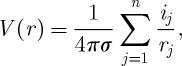2.2

where V (r) is the LFP at position r, and is generated by a set of n current sources i_j,r_j is the distance between the LFP site and each current source i_j and σ is the extracellular conductivity, which is assumed to be constant and uniform. In this widely used model, there is no frequency-filtering property due to extracellular space.

For this reason, we use a second model (model 2) that presents strong filtering properties due to the inhomogeneous structure of extracellular space. This second model considers a non-homogeneous conductivity by including spatial variations (or inhomogeneities) of both conductivity (σ) and permittivity (ε). In this case, one cannot use equation (2.2), because it is only valid if σ and ε are constant. One needs to restart from first principles (Maxwell equations) and integrate the spatial variations of these parameters. This was done previously [22], and the LFP in frequency space is given by

2.3

where V_ω is the ω frequency component of the LFP. In this equation, the conductivity (σ) and permittivity (ε) can be arbitrarily complicated functions of space. If they are constant in space, equation (2.3) reduces to the well-known Laplace equation (∇²V_ω=0), which itself leads to equation (2.2). With non-homogeneous conductivity, this model can display strong filtering properties [22].

Using this equation, assuming that the spatial variations of σ and ε follow a spherical symmetry around the current source, and that the LFP vanishes at large distances, leads to the following expression for the LFP in frequency space and at position r₀:

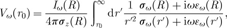2.4

where R is the radius of the source, I_ω(R) is the current produced by the source and σ_z(R) is the extracellular conductivity at the border of the spherical source. Note that, for generality, the conductivity and permittivity are written here as frequency-dependent, which is only the case for macroscopic measurements (in which case it was shown that this expression is still valid; see [32]). In the present model, however, we have considered these parameters as distance-dependent but frequency-independent.

Thus, the LFP at a position r₀ from a set of N current sources is calculated by evaluating, for each frequency,

2.5

where r_j is the position of the jth current source, and Z_ω(r_j) is the impedance given by

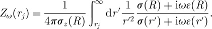2.6

These expressions must be evaluated for every current source, and the LFP is the summation of the contributions for each source.

This model was used with an exponentially decaying profile of conductivity, where the conductivity is high in the vicinity of the neuronal membrane (extracellular fluid), and decays to a minimal value, which is equal to that of the constant-resistivity model. The basis of this conductivity profile is the following. The membrane is always surrounded by a layer of conductive fluid, so the conductivity is high for short distances. The average conductivity is necessarily lower for large distances, because one averages over highly conductive fluids and low-conductivity membranes. At very large distances, the average conductivity converges to a much lower conductivity value, which was assumed to be close to the conductivity of membranes. This profile was shown to produce a low-pass frequency filtering, where action potentials attenuate much more steeply than slower processes such as synaptic potentials [22]. The same model is used here with a spatial constant of conductivity decay of 5 μm, maximal and minimal conductivity values of σ=1.56 and 1.56×10⁻⁹ S m⁻¹, respectively, and a constant permittivity of ε=7×10⁻¹⁰ F m⁻¹ (see Bedard et al. [22] for a discussion of these parameters).

3. Results

(a). Slow oscillations in the thalamocortical network model

Our network model included several cell types distributed across different cortical and thalamic layers (see §2; figure 1). In short, we simulated layer V PY neurons with soma located in layer V and apical dendrites in layer I, layer VI PY cells with somas in layer VI and primary dendrites in layer IV, and layer IV with PY cells located in layer IV. Each cortical layer included a population of inhibitory INs; cortical structures interacted with thalamic relay neurons of the matrix (projecting to superficial layers) and core (projecting to layer IV) subsystems. This model provides a dramatic simplification of the cortical structure, particularly because the two-compartment design of the cortical neurons only allows the distribution of all synapses in one specific compartment (specific spatial location). Nevertheless, this model was able to generate realistic activity patterns, and we used it to calculate the LFP profile using different approaches (§2).

Figure 2 shows a typical activity pattern generated in the network model during approximately 20 s of simulated sleep slow oscillation. In this model, spontaneous summation of miniature excitatory post-synaptic potentials (EPSPs) through AMPA-mediated synapses between cortical PY neurons (see §2) triggered Na⁺ spikes in some PY neurons, which then transmitted to their neighbours. The level of synchronization at the initiation of an active state depended on how many PY neurons generated the initial Na⁺ spike within the same short time window, how close these neurons were located within the network and, to large extent, how fast the signals propagated. The spread of activity was mediated by the lateral excitatory connections within layers and between cortical layers. A typical active state recruited every 2 s approximately, lasted between 0.5 and 1 s, and its termination depended on the activity of inhibitory INs, depression of excitatory connections and progressive activation of Ca²⁺-dependent K⁺ currents. In vivo sleep slow oscillations usually include longer active and shorter silent states [18]. Nevertheless, the pattern of activity generated with our model resembles slow oscillations recorded in vitro [5].

Figure 2.

Network activity during slow sleep. The entire network oscillated synchronously between active (up) and silent (down) states. (a) Space plot of network activity in layer IV. Dark blue colour indicates hyperpolarized potentials; light colours indicate depolarized potentials corresponding to excitatory post-synaptic potentials and action potentials. (b) Representative examples of membrane voltage (Vm) oscillations in two PY neurons (indicated by arrowheads in (a)). Spike amplitude varies because of sampling rate. (Online version in colour.)

(b). Simulated local field potential during slow oscillations

Knowledge of intrinsic and synaptic currents generated in each compartment allowed us to calculate the LFP. In short, two compartments of a single cortical neuron model represented sink and source of a current, and the sum of all intrinsic and synaptic currents in each compartment was equal to the axial current flowing between compartments (figure 3); the opposite current flowed in the extracellular space and was used to calculate the LFP. Since the amplitude of the electric field in any particular spatial location of the network depends on the network geometry, specifically on the distance between neurons and between compartments, we made an assumption that the distance between any two layers is approximately 400 μm (based on the assumption that the cortex is 2 mm thick). We also assumed that the cortical synaptic footprint covers approximately 1 mm (based on the typical size of the cortical column); thus, the distance between two neighbouring PY cells was estimated as approximately 100 μm (total network size in the X-direction was 20 mm). This estimation is about one order of magnitude larger than physiological data, but it was a necessary compromise, considering the very limited size of the simulated population of neurons and synaptic footprints. We assigned spatial coordinates (X=0, Z=0) to cell number 1 in layer I; cell number 200 in layer I had coordinates (X=20 mm, Z=0); and cell number 1 in layer VI had coordinates (X=0, Z=2 mm). Finally, to compensate for our model limitations of having synapses only in apical dendrites (e.g. layer V cells only have synapses in layer I), we used the inverted current polarity to calculate the LFP. This produced current sources in superficial layers during high network activity as observed in vivo. In a more realistic model, the same effect could be achieved by having a relatively larger fraction of synapses on basal dendrites and proximal part of apical dendrites in deep layers.

Figure 3.

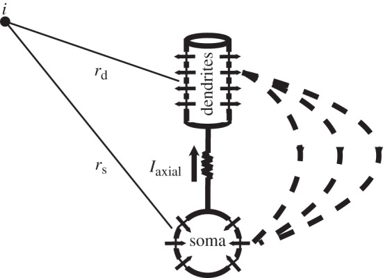
Local field potential (LFP) estimation. Each cortical neuron included two compartments. The axial current between compartments was equal and opposite to the current flowing in the extracellular space. This current was used to calculate the LFP at a specific point in space using either the constant- or variable-resistivity model.

Figure 4 shows the depth LFP profile in the middle of the network (X=10 mm) estimated from the electrical activities of all the neurons, using the assumption of current sources embedded in a uniform medium (model 1). During active states, the LFP was characterized by high-frequency oscillations, with positive bias in superficial layers (layers I–II) and negative bias in deep layers (layers V–VI). The LFP amplitude decayed quickly after active state offset and was nearly zero during the entire silent state. The corresponding CSD profile is shown at the end of this subsection. These estimations seem to be in reasonable agreement with experimental data. For example, Rappelsberger et al. [19] described negative potentials and corresponding active (mediated by depolarization) current sinks in layer V, and positive potentials and passive current sources in superficial layers during the active state of slow sleep oscillations. In Chauvette et al. [18], these current sinks in deep layers during active states were directly associated with activity and firing of layer V neurons. However, this simple LFP model showed nearly zero field potentials during silent states (figure 4b,c), and thus failed to explain the strong potentials observed in vivo during the silent states of slow oscillations [18,19]. It is important to note that rescaling resistivity by some factor cannot solve this problem. Because the model with constant resistivity is linear, rescaling resistivity amounts to rescaling the extracellular potential by the same factor. Therefore, the same graphs (figure 4b,c) can apply by only changing the amplitude calibration accordingly.

Figure 4.

LFPs for constant-resistivity model. (a) Membrane voltage of a PY cell from layer IV indicates periodic transitions between active and silent states. (b) Depth (across layers) LFP profile in the middle of the network (x= 10 mm): x-axis, time; y-axis, cortical depth. The LFP signal was low-pass filtered at 50 Hz. Layer 0 (VII) represents a location 400 μm above (below) layer I (VI). (c) Unfiltered LFP traces in layers 0–V.

We next calculated the LFP profiles using the model taking into consideration a non-homogeneous medium conductivity (model 2). Figure 5 compares the LFP generated by the two models considered in this paper in one specific location in the middle of the network (X=10 mm), one layer above layer I (Z=−400 μm). Starting from an example current source in the network (figure 5a), the impedance calculated from equation (2.6) is either frequency-dependent or constant according to which model is used (figure 5b). The extracellular potential calculated from this single source is markedly different (compare figure 5c,d). Note that the amplitude is larger for the non-homogeneous conductivity model, even though the conductivity decays with distance and thus is lower overall compared with the constant-conductivity model. This frequency-dependent attenuation of the signal is much weaker for low frequencies, which results in an LFP signal with much more power in low frequencies (compared with the constant-resistivity model), while fast frequencies (such as action potentials) are comparatively attenuated.

Figure 5.

Comparison between two models for generating LFPs. (a) Single current source from the dendrite of a layer V cell in the simulation of figure 2. (b) Impedance spectrum (square modulus) as a function of frequency for two models of LFPs, where the resistivity is either homogeneous (‘constant resistivity’) or inhomogeneous (‘variable resistivity’). A 100-fold higher value was also used (‘high’). (c,d) Extracellular potential generated by these two models applied to the current source in (a), and using an extracellular electrode located at 100 μm away from the source. (e,f) LFP generated for each model in the middle of the network (X=10 mm, Z=−400 μm) by the ensemble of neurons during slow-wave oscillations (800 current sources; see text for details). In (d,f), the two calibrations correspond to the two values used for constant conductivity, as indicated.

Figure 5e,f compares the full LFP generated by the entire network in the same conditions. The effect of the non-homogeneous conductivity is to enhance the propagation of slow frequencies over large distances, which results in an LFP profile much less dominated by multi-unit spike activity, and which bears more resemblance to the LFPs recorded experimentally.

Figure 6 shows the depth LFP profiles across all layers generated in the middle of the network (X=10 mm) using model 2. In contrast to model 1 (compare with figure 4), the LFP signals calculated assuming a non-homogeneous resistivity (model 2) showed a more complex evolution of current sink–source distribution during network transitions (figure 6b). The LFP was largely positive in superficial layers during active states, and negative in deep layers, reflecting a sink–source distribution similar to that found in vivo. The strongest low-frequency component was found in layer I. Following transition to the silent state, the LFP changed its polarity and was represented by negative potentials in superficial layers and positive potentials in deep layers. The last represented the main difference between model 2 (non-homogeneous resistivity) and model 1 (homogeneous resistivity), where the LFP was nearly zero during silent states.

Figure 6.

LFPs for variable-resistivity model. (a) Membrane voltage of a PY cell from layer IV. (b) Depth LFP profile in the middle of the network (X= 10 mm). The LFP was low-pass filtered at 50 Hz. (c) Unfiltered LFP traces in layers 0–V. Note the strong and non-uniform LFP profile during silent states of thalamocortical network (indicated by lack of spiking in PY cell from (a)).

We next calculated the depth CSD profile using the standard second-derivative approach. In both LFP models during active states, the CSD was represented by two sink–source pairs: one pair located in layers I–III and another one located in layers IV–VI (figure 7b,c). While some studies reported simpler LFP profiles during active states dominated by sources in superficial and sinks in deep layers [18,33], others found a more complex sink–source distribution [19] similar to that reported in this study. Furthermore, recent human studies described a dominant sink–source pair in superficial layers [34]. Nevertheless, all these experimental studies reported strong current sources during the silent states of slow oscillations. This structure was completely missing from our model when the LFP was calculated using the assumption of homogeneous resistivity (figure 7b). By contrast, the non-homogeneous resistivity model revealed sink–source distributions during silent states opposite to those found during active states (figure 7c), in agreement with experimental observations. This model produced an alternation of current-sink distribution in both space (cortical depth) and time, reflecting periodic network transitions between active and silent states. We also plotted the CSD profile estimated from human data (figure 7d, modified from fig. 6 of Csercsa et al. [34]; zero time corresponds to the peak of the surface positive LFP half-wave) and the CSD during one cycle of silent-to-active state transition calculated in this study using model 2 (figure 7e). The current sink–source structure was very similar in superficial layers during both silent and active states, while the model also revealed current sources in deep layers.

Figure 7.

Current-source density (CSD) analysis. (a) Membrane voltage (Vm) of a PY cell from layer IV. (b) Depth CSD profile in the middle of the network (X=10 mm) from the constant-resistivity (homogeneous media) model: x-axis, time; y-axis, cortical depth. The CSD was low-pass filtered with cutoff at 5 Hz. The CSD profile shows sink–source pairs in superficial and deep layers during active (up) states but was nearly zero across all layers during silent (down) states. (c) Depth CSD profile in the middle of the network (X= 10 mm) from the variable-resistivity (non-homogeneous media) model. The CSD profile during active states was similar to that estimated from the constant-resistivity model (b). In contrast to constant-resistivity model, the CSD was also non-uniform and non-zero during silent (down) states. (d) Depth CSD profile calculated during slow wave activity in humans (adapted from Csercsa et al. [34] with permission). Time-locked averages to the peak of the surface positive half-wave (up-state) shows alternating sink–source pair in the superficial layers. (e) CSD profile during one episode of silent–active state transition from the variable-resistivity model.

4. Discussion

In this study, we used a well-established model of sleep slow oscillations [4,10] to explore the neuronal factors behind experimental EEG and LFP signals recorded during deep sleep. We found that using a conventional constant-conductivity model, assuming that the LFP is generated by current sources embedded in a uniform resistive medium [21], may explain the in vivo distribution of current sinks and sources between the superficial and deep cortical layers during active phases of slow oscillations. However, it failed to explain the strong source distribution during silent states of slow-wave sleep [18]. An alternative model of LFP generation presented strong filtering properties due to the properties of extracellular space. This second model considered a non-homogeneous conductivity by including spatial variations (or inhomogeneities) of both conductivity and permittivity [22,32], accounting for the fact that the extracellular space is packed with different cellular processes, including fluids and membranes. This second model also produced the correct distribution of sinks and sources during active states of slow oscillations. In contrast to the first model, it generated non-zero CSD during silent states as well. These current densities during silent states were opposite to those during active states, therefore providing alternating sequences of sinks and sources in time during slow oscillations, in good agreement with experimental data [18,19,33–35].

Understanding the meaning of the EEG and LFP patterns in terms of the activity of contributing groups of neurons, as well as understanding which conclusions about the activity of specific types and groups of neurons can be drawn from analysing the EEG and LFP, remains an important and largely open problem. Clearly, the EEG is a result of changes of electrical activity of multiple sources, and ultimately represents the activity patterns of entire populations of neurons and glial cells in the brain. In contrast, the LFP provides a (relatively) microscopic measure of brain activity, summarizing the electrical activities of possibly thousands of neurons [36,37]. In large part, these activities come from the gradients of the membrane voltage between different compartments of individual cells and usually result from synaptic activation mediated by action potentials. For example, excitatory synaptic activation in a given compartment will create a flow of positive ions inside the cell (active current sink), depolarizing the intracellular space and creating a negative potential in the surrounding space. These gradients will then lead to current flow between compartments inside the membrane and in the extracellular space, and will lead to hyperpolarization of the membrane at sites where positive ions leave the cell (passive current source). Another possibility includes active current sources due to the inhibitory synaptic currents and corresponding passive current sinks. These distributions of current sinks and sources create dipoles of electrical activity, which represent a major contribution to the LFP [38–41], with recent evidence pointing to a particularly strong impact of inhibition [42–44]. In the cerebral cortex, the unique configuration, with large structurally oriented PY neurons with somas located in the deep layers and dendrites located in the superficial layers, provides a strong contribution to the measured LFP (and EEG) signals. Indeed, the strength of the electric field produced by a dipole depends on the distance between current sinks and sources [21], which makes the large PY neurons in layers V and VI the main contributors of the LFP and EEG signals.

In principle, both the slower synaptic currents and the fast intrinsic currents generated during action potential propagation contribute to the LFP. However, in part because of the low-pass filtering properties of the extracellular media [22], the high-frequency electric fields associated with action potentials are steeply attenuated, and only nearby neurons can generate significant extracellular spike signals. Therefore, the models of the LFP assuming uniform electrical properties of the extracellular medium would overestimate the contribution of fast intrinsic currents and underestimate the effect of slow synaptic and intrinsic conductances. As a result, these models will generate electrical signals that decay quickly after offset of any brain activity (such as an active state of the slow oscillations) and will produce almost no signal during even short episodes of reduced brain activation (such as during silent states of slow oscillations). In contrast, the LFP profiles measured in vivo include a strong distribution of current sinks and sources during silent states [18].

Taking into account the filtering properties of extracellular media, by including either physical processes such as ionic diffusion or inhomogeneous electrical properties [22,32], could generate LFP profiles that are in agreement with experimental data. With this approach, the effect of fast currents was diminished, while the slow intrinsic and synaptic currents provided the major contribution to the LFP signal far from neurons, a situation that is more realistic. This generated slow changes of the LFP, even between active states (during silence), and produced CSD profiles opposite to those found during active states, in agreement with experimental observations. The LFP profiles simulated in this study using non-homogeneous medium conductivity still included a relatively low-amplitude phase just before the active state onset. This, however, can be explained by the relatively long (typically around 1 s) duration of the silent states in the model (which was more in vitro-like in this respect [5]) compared with the relatively short (typically less than 0.5 s) silent states in vivo [45].

Note that the model used in Bedard et al. [22] was derived based on an assumption of spherical symmetry of the conductivity and permittivity around the source, and was applied here to a geometry that is not spherical. However, this assumption should not qualitatively alter the results of the present model because of the low density of current sources in this model (source size is 2 μm, with 100 μm distance between sources). In such conditions, we can still assume that the medium around each source is quasi-isotropic in the sense that in every direction, on average, the electrical parameters will have similar spatial variations. This suggests that the spherical symmetry of the medium around each source should still be a good approximation. Other mechanisms, such as ionic diffusion, give similar low-pass filtering properties [32]; integrating such mechanisms should, in principle, give similar results as shown here.

Finally, an important question is whether the difference found here between the two LFP models could have any potential consequence in our understanding of ephaptic (electric field) interactions. Because clearly low frequencies seem to be more impactful than expected, it is obviously a possible cause of large-scale synchrony that should be evaluated by appropriate models. Such models are not trivial, however, because the whole system, including membrane equations, must be formalized in frequency space (as in equations (2.3)–(2.6)). This constitutes a good challenge for future work.

In conclusion, we showed that taking into account the filtering properties of extracellular space is critical to explain the in vivo LFP patterns recorded during sleep slow oscillations. Furthermore, this model of LFP signals is also able to reproduce critical features of the CSD profiles, such as the CSD distribution during the down (silent) states of slow oscillation. The latter feature is not reproduced by traditional LFP models with uniform resistivity, which may mean that these traditional models are insufficient, or alternatively that our network model of up and down states is too simple. Further work is needed to investigate these questions.

References

- 1.Achermann P., Borbely A. A.1997Low-frequency (<1 Hz) oscillations in the human sleep electroencephalogram Neuroscience 81213–222. 10.1016/S0306-4522(97)00186-3 (doi:10.1016/S0306-4522(97)00186-3) [DOI] [PubMed] [Google Scholar]
- 2.Steriade M., Timofeev I., Grenier F. Natural waking and sleep states: a view from inside neocortical neurons. J. Neurophysiol. 2001;85:1969–1985. doi: 10.1152/jn.2001.85.5.1969. [DOI] [PubMed] [Google Scholar]
- 3.Timofeev I., Grenier F., Steriade M.2001Disfacilitation and active inhibition in the neocortex during the natural sleep–wake cycle: an intracellular study Proc. Natl Acad. Sci. USA 981924–1929. 10.1073/pnas.041430398 (doi:10.1073/pnas.041430398) [DOI] [PMC free article] [PubMed] [Google Scholar]
- 4.Timofeev I., Grenier F., Bazhenov M., Sejnowski T. J., Steriade M.2000Origin of slow cortical oscillations in deafferented cortical slabs Cereb. Cortex 101185–1199. 10.1093/cercor/10.12.1185 (doi:10.1093/cercor/10.12.1185) [DOI] [PubMed] [Google Scholar]
- 5.Sanchez-Vives M. V., McCormick D. A.2000Cellular and network mechanisms of rhythmic recurrent activity in neocortex Nat. Neurosci. 31027–1034. 10.1038/79848 (doi:10.1038/79848) [DOI] [PubMed] [Google Scholar]
- 6.Destexhe A.2009Self-sustained asynchronous irregular states and up–down states in thalamic, cortical and thalamocortical networks of nonlinear integrate-and-fire neurons J. Comput. Neurosci. 27493–506. 10.1007/s10827-009-0164-4 (doi:10.1007/s10827-009-0164-4) [DOI] [PubMed] [Google Scholar]
- 7.Fatt P., Katz B. Spontaneous sub-threshold activity at motor-nerve endings. J. Physiol. 1952;117:109–128. [PMC free article] [PubMed] [Google Scholar]
- 8.Paré D., Lebel E., Lang E. J. Differential impact of miniature synaptic potentials on the soma and dendrites of pyramidal neurons in vivo. J. Neurophysiol. 1997;78:1735–1739. doi: 10.1152/jn.1997.78.3.1735. [DOI] [PubMed] [Google Scholar]
- 9.Salin P. A., Prince D. A. Spontaneous GABAA receptor-mediated inhibitory currents in adult rat somatosensory cortex. J. Neurophysiol. 1996;75:1573–1588. doi: 10.1152/jn.1996.75.4.1573. [DOI] [PubMed] [Google Scholar]
- 10.Bazhenov M., Timofeev I., Steriade M., Sejnowski T. J. Model of thalamocortical slow-wave sleep oscillations and transitions to activated states. J. Neurosci. 2002;22:8691–8704. doi: 10.1523/JNEUROSCI.22-19-08691.2002. [DOI] [PMC free article] [PubMed] [Google Scholar]
- 11.Compte A., Sanchez-Vives M. V., McCormick D. A., Wang X.-J.2003Cellular and network mechanisms of slow oscillatory activity (<1 Hz) and wave propagations in a cortical network model J. Neurophysiol. 892707–2725. 10.1152/jn.00845.2002 (doi:10.1152/jn.00845.2002) [DOI] [PubMed] [Google Scholar]
- 12.Hughes S. W., Cope D. W., Blethyn K. L., Crunelli V.2002Cellular mechanisms of the slow (<1 Hz) oscillation in thalamocortical neurons in vitro Neuron 33947–958. 10.1016/S0896-6273(02)00623-2 (doi:10.1016/S0896-6273(02)00623-2) [DOI] [PubMed] [Google Scholar]
- 13.Crunelli V., Hughes S. W.2010The slow (<1 Hz) rhythm of non-REM sleep: a dialogue between three cardinal oscillators Nat. Neurosci. 139–17. 10.1038/nn.2445 (doi:10.1038/nn.2445) [DOI] [PMC free article] [PubMed] [Google Scholar]
- 14.Hill S., Tononi G.2005Modeling sleep and wakefulness in the thalamocortical system J. Neurophysiol. 931671–1698. 10.1152/jn.00915.2004 (doi:10.1152/jn.00915.2004) [DOI] [PubMed] [Google Scholar]
- 15.Volgushev M., Chauvette S., Mukovski M., Timofeev I.2006Precise long-range synchronization of activity and silence in neocortical neurons during slow-wave sleep J. Neurosci. 265665–5672. 10.1523/jneurosci.0279-06.2006 (doi:10.1523/jneurosci.0279-06.2006) [DOI] [PMC free article] [PubMed] [Google Scholar]
- 16.Krnjevic K., Dalkara T., Yim C. Synchronization of pyramidal cell firing by ephaptic currents in hippocampus in situ. Adv. Exp. Med. Biol. 1986;203:413–423. doi: 10.1007/978-1-4684-7971-3_31. [DOI] [PubMed] [Google Scholar]
- 17.Contreras D., Steriade M. Cellular basis of EEG slow rhythms: a study of dynamic corticothalamic relationships. J. Neurosci. 1995;15:604–622. doi: 10.1523/JNEUROSCI.15-01-00604.1995. [DOI] [PMC free article] [PubMed] [Google Scholar]
- 18.Chauvette S., Volgushev M., Timofeev I.2010Origin of active states in local neocortical networks during slow sleep oscillation Cereb. Cortex 202660–2674. 10.1093/cercor/bhq009 (doi:10.1093/cercor/bhq009) [DOI] [PMC free article] [PubMed] [Google Scholar]
- 19.Rappelsberger P., Pockberger H., Petsche H.1982The contribution of the cortical layers to the generation of the EEG: field potential and current source density analyses in the rabbit's visual cortex Electroencephalogr. Clin. Neurophysiol. 53254–269. 10.1016/0013-4694(82)90083-9 (doi:10.1016/0013-4694(82)90083-9) [DOI] [PubMed] [Google Scholar]
- 20.Frohlich F., McCormick D. A.2010Endogenous electric fields may guide neocortical network activity Neuron 67129–143. 10.1016/j.neuron.2010.06.005 (doi:10.1016/j.neuron.2010.06.005) [DOI] [PMC free article] [PubMed] [Google Scholar]
- 21.Nunez P. L., Srinivasan R. Electric fields of the brain. 2nd edn. Oxford, UK: Oxford University Press; 2005. [Google Scholar]
- 22.Bedard C., Kroger H., Destexhe A.2004Modeling extracellular field potentials and the frequency-filtering properties of extracellular space Biophys. J. 861829–1842. 10.1016/S0006-3495(04)74250-2 (doi:10.1016/S0006-3495(04)74250-2) [DOI] [PMC free article] [PubMed] [Google Scholar]
- 23.Mainen Z. F., Sejnowski T. J.1996Influence of dendritic structure on firing pattern in model neocortical neurons Nature 382363–366. 10.1038/382363a0 (doi:10.1038/382363a0) [DOI] [PubMed] [Google Scholar]
- 24.Alzheimer C., Schwindt P. C., Crill W. E. Modal gating of Na+ channels as a mechanism of persistent Na+ current in pyramidal neurons from rat and cat sensorimotor cortex. J. Neurosci. 1993;13:660–673. doi: 10.1523/JNEUROSCI.13-02-00660.1993. [DOI] [PMC free article] [PubMed] [Google Scholar]
- 25.Kay A. R., Sugimori M., Llinas R. Kinetic and stochastic properties of a persistent sodium current in mature guinea pig cerebellar Purkinje cells. J. Neurophysiol. 1998;80:1167–1179. doi: 10.1152/jn.1998.80.3.1167. [DOI] [PubMed] [Google Scholar]
- 26.Bazhenov M., Timofeev I., Steriade M., Sejnowski T. J. Cellular and network models for intrathalamic augmenting responses during 10-Hz stimulation. J. Neurophysiol. 1998;79:2730–2748. doi: 10.1152/jn.1998.79.5.2730. [DOI] [PubMed] [Google Scholar]
- 27.Destexhe A., Mainen Z. F., Sejnowski T. J.1994Synthesis of models for excitable membranes, synaptic transmission and neuromodulation using a common kinetic formalism J. Comput. Neurosci. 1195–230. 10.1007/BF00961734 (doi:10.1007/BF00961734) [DOI] [PubMed] [Google Scholar]
- 28.Bazhenov M., Timofeev I., Steriade M., Sejnowski T. J. Computational models of thalamocortical augmenting responses. J. Neurosci. 1998;18:6444–6465. doi: 10.1523/JNEUROSCI.18-16-06444.1998. [DOI] [PMC free article] [PubMed] [Google Scholar]
- 29.Abbott L. F., Varela J. A., Sen K., Nelson S. B.1997Synaptic depression and cortical gain control Science 275221–224. 10.1126/science.275.5297.221 (doi:10.1126/science.275.5297.221) [DOI] [PubMed] [Google Scholar]
- 30.Tsodyks M. V., Markram H.1997The neural code between neocortical pyramidal neurons depends on neurotransmitter release probability Proc. Natl Acad. Sci. USA 94719–723. 10.1073/pnas.94.2.719 (doi:10.1073/pnas.94.2.719) [DOI] [PMC free article] [PubMed] [Google Scholar]
- 31.Galarreta M., Hestrin S.1998Frequency-dependent synaptic depression and the balance of excitation and inhibition in the neocortex Nat. Neurosci. 1587–594. 10.1038/2882 (doi:10.1038/2882) [DOI] [PubMed] [Google Scholar]
- 32.Bedard C., Destexhe A.2009Macroscopic models of local field potentials and the apparent 1/f noise in brain activity Biophys. J. 962589–2603. 10.1016/j.bpj.2008.12.3951 (doi:10.1016/j.bpj.2008.12.3951) [DOI] [PMC free article] [PubMed] [Google Scholar]
- 33.Sirota A., Csicsvari J., Buhl D., Buzsaki G.2003Communication between neocortex and hippocampus during sleep in rodents Proc. Natl Acad. Sci. USA 1002065–2069. 10.1073/pnas.0437938100 (doi:10.1073/pnas.0437938100) [DOI] [PMC free article] [PubMed] [Google Scholar]
- 34.Csercsa R., et al. 2010Laminar analysis of slow wave activity in humans Brain 1332814–2829. 10.1093/brain/awq169 (doi:10.1093/brain/awq169) [DOI] [PMC free article] [PubMed] [Google Scholar]
- 35.Steriade M., Amzica F.1996Intracortical and corticothalamic coherency of fast spontaneous oscillations Proc. Natl Acad. Sci. USA 932533–2538. 10.1073/pnas.93.6.2533 (doi:10.1073/pnas.93.6.2533) [DOI] [PMC free article] [PubMed] [Google Scholar]
- 36.Niedermeyer E., Lopes da Silva F. H., editors. Electroencephalography: basic principles, clinical applications, and related fields. 5th edn. Philadelphia, PA: Lippincott Williams and Wilkins; 2005. [Google Scholar]
- 37.Katzner S., Nauhaus I., Benucci A., Bonin V., Ringach D. L., Carandini M.2009Local origin of field potentials in visual cortex Neuron 6135–41. 10.1016/j.neuron.2008.11.016 (doi:10.1016/j.neuron.2008.11.016) [DOI] [PMC free article] [PubMed] [Google Scholar]
- 38.Creutzfeldt O. D., Watanabe S., Lux H. D.1966Relations between EEG phenomena and potentials of single cortical cells. I. Evoked responses after thalamic and erpicortical stimulation Electroencephalogr. Clin. Neurophysiol. 201–18. 10.1016/0013-4694(66)90136-2 (doi:10.1016/0013-4694(66)90136-2) [DOI] [PubMed] [Google Scholar]
- 39.Creutzfeldt O. D., Watanabe S., Lux H. D.1966Relations between EEG phenomena and potentials of single cortical cells. II. Spontaneous and convulsoid activity Electroencephalogr. Clin. Neurophysiol. 2019–37. 10.1016/0013-4694(66)90137-4 (doi:10.1016/0013-4694(66)90137-4) [DOI] [PubMed] [Google Scholar]
- 40.Klee M., Rall W. Computed potentials of cortically arranged populations of neurons. J. Neurophysiol. 1977;40:647–666. doi: 10.1152/jn.1977.40.3.647. [DOI] [PubMed] [Google Scholar]
- 41.Lopes da Silva F., Van Rotterdam A. Biophysical aspects of EEG and magnetoencephalogram generation. In: Niedermeyer E., Lopes da Silva F. H., editors. Electroencephalography: basic principles, clinical applications, and related fields. 5th edn. Philadelphia, PA: Lippincott Williams and Wilkins; 2005. pp. 107–125. [Google Scholar]
- 42.Trevelyan A. J.2009The direct relationship between inhibitory currents and local field potentials J. Neurosci. 2915299–15307. 10.1523/jneurosci.2009-09.2009 (doi:10.1523/jneurosci.2009-09.2009) [DOI] [PMC free article] [PubMed] [Google Scholar]
- 43.Bazelot M., Dinocourt C., Cohen I., Miles R.2010Unitary inhibitory field potentials in the CA3 region of rat hippocampus J. Physiol. 5882077–2090. 10.1113/jphysiol.2009.185918 (doi:10.1113/jphysiol.2009.185918) [DOI] [PMC free article] [PubMed] [Google Scholar]
- 44.Oren I., Hajos N., Paulsen O.2010Identification of the current generator underlying cholinergically induced gamma frequency field potential oscillations in the hippocampal CA3 region J. Physiol. 588785–797. 10.1113/jphysiol.2009.180851 (doi:10.1113/jphysiol.2009.180851) [DOI] [PMC free article] [PubMed] [Google Scholar]
- 45.Steriade M., Nuñez A., Amzica F. A novel slow (<1 Hz) oscillation of neocortical neurons in vivo: depolarizing and hyperpolarizing components. J. Neurosci. 1993;13:3252–3265. doi: 10.1523/JNEUROSCI.13-08-03252.1993. [DOI] [PMC free article] [PubMed] [Google Scholar]