In vivo optical imaging and dynamic contrast methods for biomedical research

Abstract

This paper provides an overview of optical imaging methods commonly applied to basic research applications. Optical imaging is well suited for non-clinical use, since it can exploit an enormous range of endogenous and exogenous forms of contrast that provide information about the structure and function of tissues ranging from single cells to entire organisms. An additional benefit of optical imaging that is often under-exploited is its ability to acquire data at high speeds; a feature that enables it to not only observe static distributions of contrast, but to probe and characterize dynamic events related to physiology, disease progression and acute interventions in real time. The benefits and limitations of in vivo optical imaging for biomedical research applications are described, followed by a perspective on future applications of optical imaging for basic research centred on a recently introduced real-time imaging technique called dynamic contrast-enhanced small animal molecular imaging (DyCE).

1. Introduction

(a). Contrast mechanisms for in vivo optical imaging

In vivo optical imaging exploits contrast that interacts with visible and near-infrared wavelengths of light in living tissues. While many clinical applications of optical imaging have been explored, basic research can also benefit tremendously from imaging techniques that provide information about living tissues. Compared with other types of imaging modalities such as X-ray and magnetic resonance imaging (MRI), optical imaging has the major benefit of being able to exploit a rich palette of contrast. Endogenous contrast already present in many organisms includes the differing absorption properties of oxy- and deoxy-haemoglobin, lipids and water, as well as the intrinsic fluorescence of many substances including keratin, elastin, collagen cross-links, phospholipids, tryptophan, retinol, lipofuscin and metabolites nicotinamide adenine dinucleotide and flavin adenine dinucleotide [1–4]. These substances can provide information about both the structure and function of living tissue. Additional contrast mechanisms such as elastic and inelastic scattering can also provide valuable information about the composition and structure of tissues [5,6]. Exogenous contrast further adds to the possibilities presented by in vivo optical imaging, since an extensive and growing collection of absorbing and fluorescent forms of contrast are now compatible with in vivo use, many of which can be targeted to specific biochemical markers. These can include organic or inorganic dyes [7,8], nanoparticles [9], quantum dots [10], fluorescent proteins [11] and complex constructs that exploit properties such as Förster resonance energy transfer (FRET) to make them activatable or modulatable [12,13].

While some exogenous labelling approaches have been successfully approved for use in humans [14,15], such tools can be readily translated into non-human animals for basic research use with few hurdles to rapid implementation. An important example of this is the use of transgenic techniques that modify the DNA of cells or even a complete organism to cause them to express optical contrast with high specificity [11]. Research into diseases such as cancer has been transformed by the availability of such transgenic techniques, allowing green fluorescent protein (GFP) or its successors to target and label specific cell types in living animals. GFP variants can be made responsive to environmental changes, such as calcium or glucose concentrations via FRET mechanisms. Bioluminescence imaging [16] combines firefly genes into cells to cause them to express luciferase, which will emit light upon combination with injected luciferin. Another exciting research frontier is optogenetics, a transgenic method that causes cells to produce light-activatable ion channels, allowing specific cells in excitable tissues to be either activated or inhibited simply using light [17].

Transgenic techniques have rapidly become mainstream in basic research, and through the use of viral transfection, often no longer require time-consuming and costly generation of custom, genetically modified strains of mice, but can be quickly and easily applied in a range of species [18]. Transgenic techniques have also had a significant impact on the availability of animal models of human diseases such as cancer, Alzheimer's, diabetes and many more [19–21].

(b). Benefits of in vivo imaging for research

A major goal of basic biomedical research is to better understand the pathophysiology of human diseases, and to determine and evaluate potential therapeutics for those diseases. Traditional approaches to such research would use large cohorts of animals (often mice), which would be allowed to develop specific disease states in order to test outcomes of different treatments. However, the read-outs from such studies were generally gross dissection and tissue histology. As such, subsets of animals would be sacrificed at different time points to determine their level of disease and response to treatment. This approach is not only costly, lengthy and uses large numbers of animals, but also it decreases statistical power, since each animal is only measured once, and cannot be its own control. The variability of disease progression and treatment responses between animals must be accounted for via measurement of increased numbers of animals.

A solution to this problem is to be able to measure the disease state of an animal at multiple time points, non-destructively and therefore in vivo. In this case, the progress of disease within a single animal can be tracked, and its individual responses to treatment measured. In addition to the benefit of reduced variance relative to inter-animal comparisons, in vivo imaging offers the opportunity to observe the real-time physiology of the animal, rather than just having static post-mortem histological read-outs from processed tissue. Such measures could include challenging the physiology of the animal to observe the response of diseased tissue, exploring acute effects of drug administration or looking at the functional properties of diseased and normal tissue, such as perfusion and transport of specific substances.

While in vivo imaging is therefore very appealing for basic research applications, traditionally clinical techniques such as MRI and X-ray computed tomography (X-ray CT) are often prohibitively expensive, difficult to accommodate and provide insufficient throughput for large studies. Optical imaging provides an attractive option in this setting owing to the wide range of available forms of optical contrast, as well as the relatively low cost of optical instrumentation that can often be implemented in a simple bench-top configuration requiring no shielding, and minimal operator training.

(c). The effect of light scattering on in vivo optical imaging: resolution versus depth

In spite of the many advantages offered by in vivo optical imaging, it also presents many challenges. The most significant obstacle to implementing optical imaging in vivo is light scattering [22–25]. Elastic scattering of light will occur in almost all tissues, resulting in strong attenuation as well as loss of directionality and therefore limited ability to form high-resolution images. In X-ray imaging, X-rays pass through soft tissue relatively unimpeded, being attenuated only by bone and generating a rectilinear image on a screen. In vivo optical imaging must therefore address a trade-off between the depth to which it is able to image in tissues and the resolution of the image produced. This is illustrated in figure 1.

Figure 1.

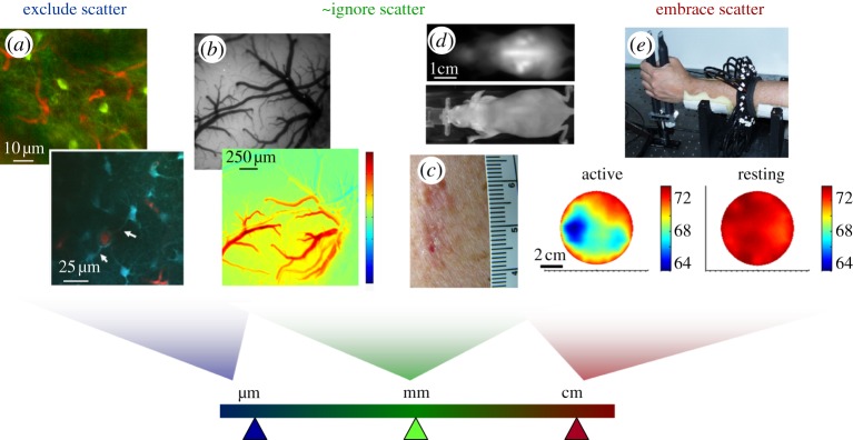
Effects of scatter on resolution for different types of in vivo optical imaging. (a) Laser scanning microscopy images (two-photon) acquired in the living rodent brain (top: green = GFP in NPY neurons, red = Texas Red dextran in capillaries; bottom: blue = SR101 in astrocytes, red = FITC dextran in vessels) [4]. For high-resolution imaging with resolution of the order of micrometres, imaging can only be achieved at depths of a few hundred micrometres where scattering effects can be excluded. (b) Top: camera-based imaging of the exposed rodent brain under 530 nm illumination; bottom: a map of the change in oxy-haemoglobin just following cessation of a 4 s hindpaw stimulus [26]. Resolution is now of the order of tens of micrometres and quantitation is affected by scattering; yet without scattering, this absorption contrast would not be measurable in a reflectance geometry. (c) Photograph of a malignant skin lesion showing haemoglobin and melanin absorption contrast. (d) Epi-fluorescence imaging (top) and white-light image (bottom) of a whole nude mouse. Organs in the mouse at depths of 2–3 mm can be seen, with resolution of the order of 1–3 mm [27]. (e) Optical tomography measurements of the human forearm, acquired by shining light all the way across 7 cm of tissue. Information about the timing of detected photons was incorporated into a diffusion model-based reconstruction to account for the effects of scattering. Images show baseline blood oxygen saturation when the arm was at rest, versus gripping a force transducer [28,29]. Through this thickness of tissue, resolution here is of the order of 1–2 cm.

Techniques such as in vivo confocal and two-photon microscopy enable high-resolution (sub-micrometre) imaging in living tissues [4,30–35]. This is achieved through the rejection of scattered light by detecting only light that has formed a tight focus within the tissue, as illustrated in figure 2a. Since this tight focus requires that the light has travelled in almost entirely straight lines through the tissue before focusing, the depth at which this focus can form is limited by the scattering density of the tissue. Many biological tissues have reduced scattering coefficients of between 3 and 0.5 mm⁻¹ in the visible to near-infrared range, and therefore have mean free paths over which light can travel before experiencing significant scattering of between 0.3 and 2 mm [36,37]. This typically limits confocal and two-photon imaging to depths of less than 300 and 600 μm, respectively [35,38,39]. To implement such high-resolution imaging techniques in vivo, it is therefore often necessary to expose the tissue of interest (e.g. via surgery or endoscopy) such that imaging optics can be positioned close to the tissue's surface, and imaging will only be possible within the superficial layers of the tissue [4]. Nevertheless, in vivo microscopy techniques have had enormous impact on basic research, particularly for imaging the living brain of rats and mice using vascular tracers [40] as well as cell-specific markers [35], transgenic proteins [13] and calcium-sensitive dyes [41,42] that allow the activity of single neurons to be visualized and recorded in parallel. In cancer research, models such as ‘dorsal skin flap’ preparations allow in vivo microscopy of tumour development and therapeutic response. In this method, a glass window is implanted into a stretched section of the skin on the back of a small animal such as a mouse, enabling the structure and function of tumours induced beneath the window to be directly and repeatedly observed at a cellular level over time [43,44]. Additional optical techniques within this category include coherent anti-Stokes Raman spectroscopy and stimulated Raman scattering microscopy, which rather than measuring fluorescence, sense vibrational resonances of a wide range of molecules. Both techniques are similar to two-photon microscopy insofar as they are nonlinear, occurring only at the focus of an incident beam, and can thus achieve optical sectioning to depths of up to 500 μm in living tissue [45,46]. Optical coherence tomography (OCT) detects light that has been backscattered from structures at a particular depth by exploiting constructive and destructive interference between the returning light and a reference beam [47,48]. Scattered light is largely rejected since constructive interference only occurs with light that has been minimally scattered thereby maintaining its coherence. OCT can image to depths of up to 2 mm. Extensions of OCT include Doppler OCT and more recently optical microangiography, which exploit the motion of objects within the tissue (usually red blood cells flowing in vessels) to extract vascular maps, as well as speeds of blood flow [49–51].

Figure 2.

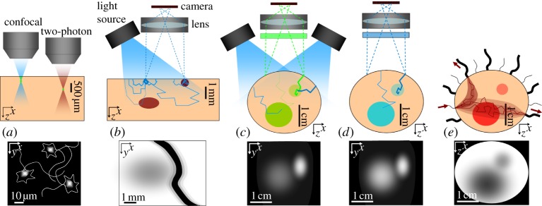
Measurement geometries, light paths and image formation. (a) Illustration of the way that laser scanning microscopy eliminates scattering to obtain higher resolution. At a depth where the focus can no longer form, no image will be seen. (b) The measurement geometry for figure 1b. Thicker lines represent the paths of light that are less likely to have been absorbed. A large fraction of detected light will have only probed the very surface. Some light will probe deeper objects, but contribute less to the detected signal than light that has travelled superficially, and will also scatter and therefore blur more. Surface absorbing objects will therefore appear much darker and more clearly defined than deeper ones, although edge effects on superficial objects can also occur. (c) Fluorescent inclusions in a non-fluorescent background in a configuration similar to that used for figure 1d. While all detected green light must have come from the fluorescent regions, more superficial regions will receive more excitation light, and more emitted light from these regions will reach the detector. Deeper regions may be below the detection limit of the camera, especially if superficial fluorescence fills the camera's dynamic range. (d) Bioluminescence faces similar challenges, but attenuation of excitation light is not a factor, so deeper objects may appear brighter than would an equivalent fluorescent object. (e) Illustration of a common measurement geometry for diffuse optical tomography in which light is incident at discrete, sequential locations (usually delivered by optical fibres or a scanned laser beam), and detected at multiple positions in parallel to create tomographic datasets. Cross-sectional images can be generated using model-based reconstruction algorithms.

Despite their many benefits, high-resolution imaging methods that largely exclude scattered light, such as confocal and two-photon microscopy and OCT [52], are often insensitive to absorption contrast. This is because these techniques ensure that detected light has travelled only very short distances through the tissue (giving it a so-called short pathlength). OCT cannot easily measure fluorescence contrast, since detected light must maintain its coherence with respect to incident light. An effective way of measuring absorbing and fluorescent contrast in superficial tissues, with lower spatial resolution, is to simply illuminate the tissue, and image the emerging diffusely reflected light with a camera (as shown in figure 1b, from the surface of the rodent brain [26,53,54], and figure 1c, showing a malignant skin lesion on the face). This kind of imaging no longer has cellular resolution, but absorption from haemoglobin and melanin is clearly visible because the detected light has scattered into the tissue, increasing the average pathlength of the light detected [4]. While such images are most strongly weighted to the most superficial layer of the tissue being imaged, they do contain information about absorption contrast in deeper layers, as illustrated in figure 2b. The depth to which such measurements are sensitive, and the relative contributions from superficial and deep layers, are a function of the baseline absorbing and scattering properties of the tissue.

Similar imaging can be performed on larger volumes of tissue, for example, on an intact, nude mouse positioned under distributed illumination and imaged using a camera (figure 1d). Where absorption contrast is being imaged (i.e. the light detected is diffusely reflected and is the same wavelength as incident light), measurement sensitivity will remain superficial (as in figure 2b). However, if fluorescence contrast is being imaged, different factors contribute to depth- sensitivity. This is because in fluorescence imaging, fluorescence emission light will only be detected from regions of the tissue that contain a fluorophore. If a fluorophore is uniformly distributed within all tissue, depth sensitivity will be similar to reflectance imaging [55,56]. However, if, say, a fluorophore is present only in the kidney, 3–4 mm below the surface of the skin on a mouse's back, it is likely to be detectable owing to a lack of a larger signal from superficial layers. However, the signal will only be detected if both excitation and emission light are not excessively attenuated, and fluorescence quantum yield is high enough to meet the sensitivity limits of the camera or other detector. If the fluorophore (or tissue autofluorescence with similar spectral properties) is also present in overlying tissues, it may overwhelm or be indistinguishable from deeper signals, as illustrated in figure 2c [27].

The resolution of the detected ‘image’ of the kidney will depend on its depth and the absorbing and scattering properties of the overlying tissues at the dye's excitation and emission wavelengths, but will be of the order of 1–3 mm. As a result, although such imaging can often detect the presence of isolated fluorescent regions, interpretation and quantitation are far more challenging. For example, if a tumour is fluorescently tagged, but is growing only in axial extent, light from the most superficial part of the tumour will contribute much more to the detected signal than light travelling from deeper parts of the tumour. Therefore, while the tumour volume might double over time, the detected signal may only change slightly. Or similarly, a small superficial lesion could prevent detection of an underlying deeper, larger lesion. The same limitations also affect bioluminescence imaging, although compared with epi-illumination geometries, deeper regions may exhibit more contrast since attenuation of excitation light (which is not required for bioluminescence) is not a factor (as illustrated in figure 2d).

These difficulties have led many researchers to use xenograft models, in which tumours are grown subcutaneously rather than in their normal anatomical location (e.g. in the colon, lung or liver), thereby reducing the impact of depth on quantitation [57,58]. However, such models often result in unrealistic growth, behaviour and cellular composition of tumours that are not in their normal biochemical and mechanical environment, making them unreliable compared with orthotopic models [59,60].

Figure 1e shows time-resolved optical tomography results acquired by transilluminating the human adult arm using pulsed near-infrared light and measuring the time taken for that light to reach detectors positioned around the arm [28]. The internal structure of changes in absorption contrast in the arm can be reconstructed from numerous measurements that project through the arm in different directions, similar to a CT scan. This is implemented as shown in figure 2e, usually with multiple optical fibres positioned on the tissue to specifically and sequentially illuminate at different discrete locations, causing detected light to pass through more clearly defined paths than for wide-field illumination [61]. This approach can also be implemented with discrete non-contact illumination such as from a steered laser beam combined with de-scanned or wide-field detection [62–64]. In contrast to CT, however, since light is so heavily scattered, reconstruction must use a model of light scattering to predict the likely paths of light through the tissue in order to estimate its internal structure [29,65]. The information that is lost as the light changes direction multiple times within the tissue causes this method to have intrinsically low resolution, which scales with the number of scattering events that have occurred and hence the overall size and optical properties of the object being imaged. For an object similar in size to the arm, or the whole newborn infant head [66], optical imaging is unlikely to provide resolution better than 0.5–1 cm. Optical tomographic imaging can be achieved for both absorbing and fluorescence contrast [67,68]. Applications of diffuse optical tomography (DOT) that are currently under development include imaging of the adult breast for lesion detection or monitoring of treatment response [69], and functional imaging of the human cortex through the intact skull and scalp [70,71]. DOT can be implemented using continuous-wave [72], time-resolved [61] or frequency-domain instrumentation [73]. Methods to improve DOT imaging performance by incorporating multi-modality information such as from X-ray, X-ray CT and MRI are also being explored [74,75].

Transillumination and tomographic reconstruction approaches can be applied for small animal imaging problems [12,76,77]. If data acquisition and modelling of light propagation could be accurately and exactly achieved, three-dimensional images of fluorescently labelled regions could feasibly be generated with spatial resolutions of the order of 2–4 mm. This better resolution is achievable because of the smaller size of mice, which reduces levels of attenuation and the extent of scattering compared with larger objects such as the human arm, breast or brain. However, in practice, acquiring and calibrating in vivo measurements and accurately modelling the complex baseline absorption and scattering properties of a whole mouse still present many challenges, leading to uncertain improvements in quantitation and resolution [78].

Overall, implementing in vivo optical imaging for research applications is a trade-off between the resolution required, access to the tissues to be imaged and the need for acute versus longitudinal measurements. For the remainder of this article, we will focus on a recently introduced method known as dynamic contrast-enhanced small animal imaging (DyCE) [27], and the benefits that it can provide with simple and efficient implementation.

2. Small animal molecular imaging approaches and challenges

As a result of the opportunities and limitations described above, so-called ‘small animal molecular imaging’ using light has been adopted in a number of different configurations for research use. Sharing the commonality that each method is designed to image an intact living mouse, these systems exploit either fluorescence or bioluminescence contrast. Current common applications of in vivo small animal imaging include

• — examination of disease progression or tumour growth and reduction in response to treatment using transfected contrast such as fluorescent proteins and luciferase [79–81], or targeted or specific contrast agents [12,82];

• — testing of contrast agents that are designed to specifically target tissues of a particular type, possibly with the intention of using non-optical labels such as radionucleotide or MRI contrast agents for clinical translation once specificity is optimized [12,57]; and

• — using labelled substances to determine targeting specificity to ultimately deliver therapies (so-called ‘theranostics’) [83,84].

As will be described further below, DyCE extends the approaches above to allow perfusion, and biodistribution and pharmacokinetics of labelled substances to be explored in vivo in the intact mouse [27,85,86]. Currently available commercial devices for small animal molecular imaging include those with epi-fluorescence geometries (e.g. the CRi/Caliper Maestro, which includes DyCE capabilities, the Kodak Carestream in vivo FX and the Xenogen/Caliper IVIS series) and tomographic imaging approaches (e.g. ART Optix MX3 and Visen/Perkin Elmer FMT 3D, Xenogen/Caliper IVIS Spectrum).

The simplest implementations of small animal optical imaging systems consist of a light source, or an array of light sources epi-illuminating a mouse, and a camera that captures images of the mouse through appropriately matched filters. In the case of bioluminescence imaging, systems can be as simple as a sensitive camera housed in a light-tight box. Tomographic implementations can be more complex, ranging from scanning the position of a laser beam over a mouse and detecting either backscattered or transmitted light, to requiring the mouse to be rotated on its long axis [87], immersed in a scattering matching fluid [77] or sandwiched between two clear plates [76]. Despite these different approaches, almost all systems face the following major challenges.

• — The impact of zero-background contrast. From an image formation stand-point, it is beneficial to have the signal only originating from the targeted region (e.g. from fluorescence or bioluminescence). However, this means that images can appear simply as a bright region against a completely dark background (figure 3a). Such data can be merged with a ‘white-light’ image of the mouse (inset), but this does not put the detected signal into the context of its anatomical location or proximity to specific organs. Several solutions to this problem have been proposed, including combining optical imaging with other modalities such as X-ray [88] or X-ray CT [77]. However, these multi-modal approaches begin to obviate the benefits of optical imaging as a relatively inexpensive and fast bench-top method.

• — Specificity of labelling. In order to obtain such zero-background measurements, labelling of the targeted region must be highly specific. This could be achieved through local genetic expression of optical contrast (e.g. GFP and luciferase), ‘activatable’ dyes that use FRET to generate fluorescence only in the presence of a specifically targeted biomolecule [12], and contrast agents that are targeted to a specific region, organ or tissue type, which need time to build up and accumulate in target tissues while washing out from surrounding tissues. This can make imaging results unreliable and time-consuming to acquire.

• — Effects of autofluorescence. The intrinsic fluorescence of many endogenous biological molecules means that even when an animal has no artificial contrast introduced, fluorescence images (particularly at lower excitation wavelengths between 400 and 600 nm) will show fluorescence from the skin and often the gut [89,90] (figure 3). This interference between intrinsic fluorescence and the signal of interest can make high-contrast imaging very challenging, particularly at visible wavelengths where tissue absorption and scattering are also much higher, limiting penetration of light into the animal and therefore sensitivity to deeper tissues as well as achievable resolution. These challenges have made non-invasive imaging of GFP in anything other than very superficial tissues highly challenging [80]. Autofluorescence at near-infrared wavelengths (above 650 nm) is much weaker, and with reduced scattering and absorption, improved penetration depths and resolution can be achieved. A growing number of contrast agents are now available in this ‘red-shifted’ region of the spectrum as shown in figure 3 [91–93]. Multi-spectral unmixing approaches have also achieved some success in delineating target contrast from spectrally similar (but not identical) autofluorescence backgrounds, but cannot fully overcome the impact of attenuation and dynamic range at lower visible wavelengths [90].

Figure 3.

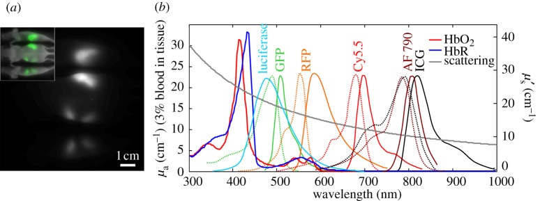
Autofluorescence, haemoglobin absorption spectra and scattering compared with common fluorescent dye spectra. (a) A three-view image of a nude mouse acquired with 570±20 nm excitation and 600 nm long-pass emission. Inset shows the signal colour-coded green and overlaid on a white-light image. No dye was administered; image shows autofluorescence from food in the intestines. (b) Absorption spectra of oxy- and deoxy-haemoglobin (HbO₂ and HbR), luciferase emission, and excitation (dots) and emission (solid) spectra of common fluorophores (GFP/RFP = green/red fluorescent protein, AF790 = Alexa-Fluor 790, ICG = indocyanine green (Invitrogen)) [13,14]. Reduced scattering spectrum is approximated using: μ′_s = Aλ^−b, where A=1.14×10⁻⁷m^(b−1) and b=1.3 [15].

(a). Quantitation

As described above, light scattering causes spatially variant sensitivity and resolution in all optical imaging approaches. More complex tomographic approaches seek to account for these variations using modelling based on estimates of the optical properties of the animal, but still have limitations on the accuracy of measured values for both signal intensity (indicating the number of fluorescent molecules present) and spatial extent (indicating the physical size of the labelled region). Tomographic approaches also require complex measurement geometries as mentioned above, meaning that they have not been widely adopted owing to the complexities of reliable data acquisition and image reconstruction. Epi-illumination fluorescence approaches do not typically attempt to provide absolute quantitation, but can be used fairly well to detect trends in signals, for example as a tumour grows, assuming that potentially confounding variables such as mouse weight gain or loss can be compensated for. An interesting approach applied to bioluminescence imaging is to use modifications in the spectral shape of the luciferase spectrum to infer the distance over which light has travelled through tissue containing haemoglobin. Since haemoglobin has distinctive absorption peaks overlapping with luciferase emission (figure 3b), the depth of a labelled region can be estimated from the luciferase spectral distortion [94,95]. However, this approach again relies on a large number of approximations.

3. Dynamic contrast-enhanced small animal molecular imaging

DyCE is a recently developed technique that overcomes many of the challenges described above, while introducing a range of new possibilities for in vivo small animal imaging [27]. DyCE refers to acquiring a time series of imaging data rather than a single, static image. While static images seek to record the final distribution of a particular contrast agent, DyCE can capture a range of different aspects of a contrast agent's interaction with tissues. For example, if a bolus of a contrast agent is delivered to the tail vein of an anaesthetized mouse, and a stream of images of the mouse are acquired over the following 100 s, the first signals observed will be at the tail and then in the heart owing to the direct route of blood flow from the tail vein to the right side of the heart as shown in figure 4a. The dye will then pass to the lungs (figure 4b), back to the heart and then up and down the ascending and descending aortas to the brain and kidneys, respectively (figure 4c). Flow through the small intestine can also usually be observed. After several passes of the bolus through the vascular system (10–20 s), a second set of dynamics begins to dominate, dictated by the contrast agent's affinity for specific tissue types. For example, if an agent crosses the blood–brain barrier, it will be observed to be gradually increasing in the brain, whereas if it does not cross, after an initial peak with the first pass of the bolus, the signal will begin to decrease (figure 4e). If the contrast agent is targeted to a tumour, contrast in that region should increase more rapidly than contrast in normal, surrounding tissue. If the dye is cleared through the liver or kidneys, this excretion pathway will be observed (figure 4d). Such rich datasets can be analysed in a host of ways to extract parameters related to perfusion, biodistribution, pharmacokinetics, tissue metabolism and physiology [96,97]. When using DyCE, it becomes important to design both contrast agents and experimental paradigms, where the dynamics of the contrast are more important than its ability to clear rapidly and absolutely from non-targeted tissues.

Figure 4.

Dynamic contrast after tail-vein bolus injection of indocyanine green (ICG). (a–d) Image frames from the time series acquired using a CRi Maestro imaging system. Time courses in (e) are extracted from regions of the raw data and show the initial circulations of the bolus of the dye through the different organs (baseline-subtracted). The signals from the heart and lungs increase early. Strong uptake in the liver can be clearly observed within 10 s. (f) Colour-coded ‘temporally unmixed’ data, where different temporal components were isolated, colour coded and overlaid to show the animal's anatomy. Colours correspond to legends on the plot. Dye dose was 0.06 ml of a 260 μM solution of ICG in distilled water.

(a). Anatomical mapping

DyCE addresses the problem of zero-background imaging by providing accurate and readily produced anatomical maps of a mouse. We have demonstrated that this can be achieved by giving a small tail-vein injection of a near-infrared dye called indocyanine green (ICG; figure 3b). A time sequence of images following a bolus injection can be analysed by seeking pixels in the time series that have distinctly different dynamics. For example, all pixels corresponding to the heart should have a rapid initial increase in intensity. By identifying pixels with this unique temporal signature and colour coding them, we can identify the location of the heart in the animal. Similarly, a wide range of other organs can be delineated within the same dataset, leading to maps like that shown in figure 4f [27]. Resolution is good because of the use of a near-infrared dye, but also because of the ability of the technique to resolve two objects that are closer to each other than their point spread function (such as the spleen and kidney) because each can be uniquely separated from the other based on the timing of the detected signals [98]. Even if two organs overlap spatially (for example, the lungs and heart in figure 4f), their time-dependent intensity traces can be unmixed, and thus signals from each organ can be extracted without cross-talk, as long as there is sufficient intensity and acceptable noise statistics. These two regions would not be resolvable from each other if they were imaged at steady state, following the same principle as modern super-resolution microscopy [99].

While anatomical maps produced using DyCE will not have resolutions equivalent to X-ray or MRI, this is in fact a direct advantage for anatomical registration with other targeted optical contrast measurements. This is because DyCE maps demonstrate the positions at which signals from particular organs will appear on an optical image of the mouse. Therefore, if a mouse is first imaged to obtain a ‘zero-background’ image of a labelled tumour in the kidney, a subsequent DyCE image (assuming similar excitation and emission wavelengths are used) will directly overlay with the original image to show whether the signal is indeed coming from the kidney, even if scatter-induced blurring or absorption-mediated distortion is present. Since X-ray, CT or MRI measurements do not have the same image-formation mechanisms, it would take significant modelling and approximations to infer exactly where and how specific anatomical structures would appear on an optical image. Furthermore, DyCE anatomical maps can be acquired without repositioning or moving the animal, as is often required for multi-modal acquisition, which means that anatomical maps are directly customized to the animal's position.

(b). Further applications of DyCE

(i). Disease delineation

Abnormal anatomical or physiological conditions are likely to alter time courses of a contrast agent following injection, compared with normal animals. If there are physical differences in vascularity and perfusion of a particular region, these disturbances are likely to affect the early phases of bolus circulation, where DyCE captures the initial inflow of the dye and its circulation around the body (as shown in figure 4). After this initial circulation phase, however, DyCE will capture additional information in later phases related to differences in the transport of the dye from the blood stream, the dye's subsequent interaction with tissues and cells and eventually its break-down or excretion pathway. Data illustrating these two phases are shown in figure 5.

Figure 5.

Simplified analysis and early/late phases of DyCE. These DyCE data were acquired using the system shown in figure 6. Rather than unmixing, organs can be clearly visualized simply by colour-merging four different image frames acquired at (a) 1.5 s, (b) 2.1 s, (c) 35 s and (d) 700 s after intravenous injection of ICG. The merge of these coloured frames shown in (e) reveals major organs including the brain (blue), lungs (cyan), liver (yellow), spleen (red), kidneys (magenta) and bile duct (green). Time courses extracted from the raw images for selected organs are shown in (f) for early phase wash-in dynamics and (g) for later phase wash-out dynamics. The green trace shows the gradual excretion of ICG from the liver into the small intestine via the bile duct corresponding to the gradual decrease of the signal in the liver (shown in yellow). The bile duct signal variations depict the pumping motion that can be readily observed along this path in the raw movie of this data. Electronic supplementary material includes a movie of the first 60 s of this image time series after removal of breathing motion.

In a recent study using DyCE of ICG circulation, combined analysis of dye inflow, uptake and wash-out was shown to be able to distinguish changes in kidney tumours in response to antiangiogenic therapy [86,100]. Another recent study used DyCE to explore the uptake dynamics of a different contrast agent (NIR-labelled 2-deoxyglucose (IRDye800CW 2-DG)) in brain tumours [85]. Differences in the uptake of this fluorescent glucose analogue in orthotopic gliomas were observed. Since ICG is strongly taken up by the liver, DyCE with ICG provides an excellent method for non-invasive evaluation of liver function [101,102]. Preliminary data from our laboratory also suggest that liver tumours exhibit distinctly different ICG uptake rates than the surrounding normal liver, allowing detection and delineation of diseased regions.

Using temporal signatures as biomarkers of pathologies provides an alternative or additional measure compared with simple fluorescence intensity measurements, potentially providing improved detection and quantitation. DyCE-derived anatomical information, which can generally be extracted from any DyCE dataset, could also allow post hoc correction of measured data via more realistic and constrained optical modelling to infer the true depth, location and concentration of a fluorescent label.

(ii). Biodistribution and pharmacokinetic analysis

DyCE can also be used to explore the biodistribution and pharmacokinetic properties of contrast agents or other labelled substances. Both the specificity and fate of new contrast agents can be readily determined using DyCE, and evaluation of the in vivo spatio-temporal dynamics of fluorescently tagged drugs or other agents could elucidate their pathways and mechanisms of action. In a recent study, DyCE was used to demonstrate the biodistribution dynamics and imaging performance of single-walled carbon nanotubes as deeper infrared in vivo contrast agents [98].

(iii). Contrast enhancement

DyCE can also be used to simply improve imaging of targeted contrast agents; firstly, allowing imaging prior to complete clearance of the agent from the body, since areas where uptake is occurring should be simple to delineate from normal or wash-out regions, thereby enhancing specificity and improving estimates of uptake kinetics. Similarly, effects of autofluorescence can be removed in a fashion similar to conventional multi-spectral unmixing, in that autofluorescence would remain constant throughout imaging and therefore be a different temporal component to the dynamically changing contrast agent.

(iv). Alternative perturbations and imaging geometries

Further extensions of DyCE reach beyond measuring the behaviour of directly injected substances. The dynamics of activatable probes may provide valuable information [12], along with the dynamics of light production after injection of luciferin in luciferase-positive animals [16]. Contrast agents or labelled substances could be inhaled or injected [103], or changes could be evoked by some other factor such as the temperature of the animal, or a surgical or pharmaceutical intervention, such as occlusion of the middle cerebral artery to explore stroke. Additional extensions of DyCE include applying DyCE analysis techniques to data that are not acquired in an epi-illumination geometry. Assuming that tomographic imaging data can be acquired rapidly enough to obtain a useful time course, DyCE analysis can be performed in either measurement or reconstructed image space to allow three-dimensional DyCE [104–106].

It is important to recognize that dynamic contrast has been successfully exploited in a number of clinical imaging modalities in an analogous way to DyCE, including dynamic contrast-enhanced MRI, X-ray CT and positron emission tomography (PET) [107–111]. Established applications, analysis techniques and imaging strategies for these dynamic modalities are therefore relevant to DyCE. However, while capable of providing kinetic parameters and/or enhanced contrast that can delineate diseased tissue, volume-acquisition rates of these modalities are generally limited. Dynamic analysis using these modalities therefore generally focuses on single organs, or parts of organs, at relatively slow time scales of the order of minutes per scan time point. Available contrast agents (such as gadolinium) are also less prone to functional interactions with tissues, remaining either in the blood stream or in the extracellular space (as in early phases of DyCE), rather than interacting with specific cell types (as in later phases of DyCE), thereby limiting the amount of specific functional information that can be extracted. Optical DyCE has the advantage that it is well suited for use in small animals, requiring no additional imaging instrumentation besides conventional light sources and a camera, and is therefore inexpensive and efficient to execute compared with MRI, PET and X-ray modalities. Motion artefacts are simpler to correct for, and there are fewer trade-offs between field of view, spatial and temporal resolution, with DyCE frame rates able to exceed 50 Hz. DyCE can also be implemented with wider ranges of contrast agents, including those that functionally interact with specific tissue types in later phases, thereby directly probing their function.

Dynamic optical imaging of intrinsic absorption contrast in the human breast has also been explored using DOT during breath-hold manoeuvres [112]. The absorption and fluorescence dynamics of intravenous ICG dye have also been measured clinically to explore enhancement of breast tumour contrast using DOT [113] and for evaluation of brain blood flow and the effects of stroke using near-infrared spectroscopy measurements [114–116]. These clinical applications illustrate the broad utility of dynamic optical contrast for extraction of functional and perfusion parameters from living tissue. DyCE extends these previous studies by also taking advantage of the improvements in imaging contrast and resolution that spatio-temporal analysis can provide in small animals.

(c). Practical considerations for DyCE imaging

The data shown in figure 4 were acquired using a CRi Maestro I system, although DyCE data can be acquired using almost any system consisting of a suitable light source and a detector array capable of acquiring a sequences of images. Figure 6 shows a typical configuration for acquisition of DyCE data. We typically arrange two mirrors on either side of the mouse to capture both overhead and side views of the mouse within the same dynamic time course, allowing visualization of more organs. Illumination is provided by either a filtered broadband light source or laser diodes, although suitably filtered light-emitting diodes could also be used. A filter in front of the camera rejects excitation light. The mouse is positioned on a small homoeothermic heat pad to maintain body temperature.

Figure 6.

A typical configuration for acquisition of DyCE data. The animal sits on a homoeothermic pad between two 45^° mirrors to allow signals from three sides of the animal to be acquired in parallel. Laser diodes (or other light sources) are positioned to evenly illuminate the mouse, and a camera with an appropriate emission filter to block excitation light is positioned above so that the animal is in focus. Adapted from Hillman & Moore [27].

In our experiments, mice are typically anaesthetized using isoflurane via a nose cone in a 1 : 3 mixture of oxygen in air. Care should be taken to use an anaesthetic that is well tolerated, and from which animals can recover for longitudinal measurements. Tail-vein injections must be performed in situ and can be achieved via either direct injection or prior placement of a venous cannula. The bolus should be delivered after image acquisition has begun. Digitally logging the time of the injection is beneficial, but it is generally simple to determine when the bolus was delivered by looking at the timing of fluorescence signals in the animal's tail. Warming the tail prior to injection using a tied latex glove filled with approximately 65^°C water helps to dilate its vessels. Aseptic techniques should be used for repeated studies and to ensure continued integrity of the tail vein. For best results, we have found that anaesthesia time should be kept to a safe minimum, and tail-vein injection should be re-attempted only once or twice before the animal is allowed to recover. We typically use nude SKH1 mice to avoid having to image through hair, although we have successfully used depilatory creams following fur clipping to expose areas of interest in other mouse strains.

We generally acquire DyCE data at around 10 frames per second in 180 s epochs. These capture the first influx of dye bolus circulation, and a moderate amount of dye uptake and wash-out. In some studies, three to five repeats of this 180 s epoch are acquired to evaluate parameters such as liver clearance dynamics (figure 5). Following data acquisition, we typically apply a correction to the data to remove the effects of breathing-related motion artefacts. This can be achieved in a number of ways, including non-rigid transformation [117]. However, we have found that mice under isoflurane anaesthesia take fairly infrequent, sharp breaths (out–in), and that the thresholding signal extracted from a region near the lungs allows frames when breaths are occurring to be identified and removed. Data are then interpolated back onto the original time-base. Without breathing correction, the dynamic motion of specific regions caused by breathing may be incorrectly interpreted as a true DyCE signal.

DyCE analysis can also be performed in a number of ways. In the simplest case, it is possible to assemble colour-coded images of major organs (lungs, kidney, liver) by extracting images from early, middle and late sections of the time course. This is shown in figure 5a–e. Principal component analysis (PCA) is a simple way to screen data for its spatio-temporal content, and will generate image components corresponding to the most common orthogonal time courses [27,98,105]. Alternative techniques include independent component analysis (ICA) [106], and blind source separation approaches [118]. For anatomical mapping, such results should be treated carefully, however, since temporal components extracted using these methods will not necessarily wholly represent a particular region's time course, and different datasets may yield similar features in different components, or might yield positive or negative components that could be misleading. As a first step, however, PCA or ICA can show quickly what the main features of the data are, and guide selection of regions of the image for manual extraction of temporal information.

For pharmacokinetic analysis, time courses can simply be extracted from target regions of the dynamic image series (guided by organ locations from PCA, for example), as shown in figures 4e and 5f,g. Returning to image-space, if a range of time courses are selected from image regions, non-negative least-squares fitting to those ‘basis time courses’ can then be used to identify all pixels with similar temporal characteristics, generating more complete and specific maps delineating different specific regions [27,119]. More complex machine-learning approaches are also being developed for DyCE analysis [120]. It is interesting to note that algorithms designed for hyperspectral unmixing can be readily applied to DyCE data (switching wavelength for time points). The composite shown in figure 4f was derived using a modified version of automated hyperspectral unmixing software routinely used in the CRi Maestro system. A further extension of DyCE analysis could incorporate pharmacokinetic models to directly extract parameters from imaging data [96,121].

DyCE images can be displayed in a number of ways. Colour-merging allows different temporal components to be overlaid to allow appreciation of the positions and overlap of different regions with respect to each other. However, since colour-merges can lead to uncertainty when more than three basic colours are used, it is advisable to visualize data in a graphical user interface environment that allows different components to be overlaid and visualized in different combinations.

4. Summary and conclusions

This paper detailed many of the great many benefits offered by optical imaging for in vivo applications related to basic biomedical research questions, rather than direct clinical translation. The different types of optical contrast that can be exploited for in vivo imaging were discussed, along with the limitations imposed by scattering. The importance of these factors for longitudinal, non-invasive small animal imaging was described, along with the major challenges faced by common approaches. Finally, DyCE was described, along with the benefits and future potential of this technique.

References

- 1.Ramanujam N. Fluorescence spectroscopy in vivo. In: Meyers R. A., editor. Encyclopedia of analytical chemistry. vol. 1. Chichester, UK: John Wiley & Sons; 2000. pp. 20–56. [Google Scholar]
- 2.Cerussi A. E., Berger A. J., Bevilacqua F., Shah N., Jakubowski D., Butler J., Holcombe R. F., Tromberg B. J.2001Sources of absorption and scattering contrast for near-infrared optical mammography Acad. Radiol. 8211–218. 10.1016/S1076-6332(03)80529-9 (doi:10.1016/S1076-6332(03)80529-9) [DOI] [PubMed] [Google Scholar]
- 3.Zipfel W. R., Williams R. M., Christie R., Nikitin A. Y., Hyman B. T., Webb W. W.2003Live tissue intrinsic emission microscopy using multiphoton-excited native fluorescence and second harmonic generation Proc. Natl Acad. Sci. USA 1007075–7080. 10.1073/pnas.0832308100 (doi:10.1073/pnas.0832308100) [DOI] [PMC free article] [PubMed] [Google Scholar]
- 4.Hillman E. M. C.2007Optical brain imaging in vivo: techniques and applications from animal to man J. Biomed. Opt. 12051402. 10.1117/1.2789693 (doi:10.1117/1.2789693) [DOI] [PMC free article] [PubMed] [Google Scholar]
- 5.Mahadevan-Jansen A., Richards-Kortum R. R.1996Raman spectroscopy for the detection of cancers and precancers J. Biomed. Opt. 131–70. 10.1117/12.227815 (doi:10.1117/12.227815) [DOI] [PubMed] [Google Scholar]
- 6.Freudiger C. W., Min W., Holtom G. R., Xu B., Dantus M., Xie X. S.2011Highly specific label-free molecular imaging with spectrally tailored excitation-stimulated Raman scattering (STE-SRS) microscopy Nat. Photon. 5103–109. 10.1038/nphoton.2010.294 (doi:10.1038/nphoton.2010.294) [DOI] [PMC free article] [PubMed] [Google Scholar]
- 7.Landsman M. L., Kwant G., Mook G. A., Zijlstra W. G. Light-absorbing properties, stability, and spectral stabilization of indocyanine green. J. Appl. Physiol. 1976;40:575–583. doi: 10.1152/jappl.1976.40.4.575. [DOI] [PubMed] [Google Scholar]
- 8.Bloch S., Lesage F., McIntosh L., Gandjbakhche A., Liang K., Achilefu S.2005Whole-body fluorescence lifetime imaging of a tumor-targeted near-infrared molecular probe in mice J. Biomed. Opt. 10054003. 10.1117/1.2070148 (doi:10.1117/1.2070148) [DOI] [PubMed] [Google Scholar]
- 9.Altinoglu E. I., Russin T. J., Kaiser J. M., Barth B. M., Eklund P. C., Kester M., Adair J. H.2008Near-infrared emitting fluorophore-doped calcium phosphate nanoparticles for in vivo imaging of human breast cancer ACS Nano 22075–2084. 10.1021/nn800448r (doi:10.1021/nn800448r) [DOI] [PubMed] [Google Scholar]
- 10.Michalet X., Pinaud F. F., Bentolila L. A., Tsay J. M., Doose S., Li J. J., Sundaresan G., Wu A. M., Gambhir S. S., Weiss S.2005Quantum dots for live cells, in vivo imaging and diagnostics Science 307538–544. 10.1126/science.1104274 (doi:10.1126/science.1104274) [DOI] [PMC free article] [PubMed] [Google Scholar]
- 11.Chalfie M., Tu Y., Euskirchen G., Ward W. W., Prasher D. C.1994Green fluorescent protein as a marker for gene expression Science 263802–805. 10.1126/science.8303295 (doi:10.1126/science.8303295) [DOI] [PubMed] [Google Scholar]
- 12.Ntziachristos V., Tung C.-H., Bremer C., Weissleder R.2002Fluorescence molecular tomography resolves protease activity in vivo Nat. Med. 8757–761. 10.1038/nm729 (doi:10.1038/nm729) [DOI] [PubMed] [Google Scholar]
- 13.Heim N., Garaschuk O., Friedrich M. W., Mank M., Milos R. I., Kovalchuk Y., Konnerth A., Griesbeck O.2007Improved calcium imaging in transgenic mice expressing a troponin C-based biosensor Nat. Methods 4127–129. 10.1038/nmeth1009 (doi:10.1038/nmeth1009) [DOI] [PubMed] [Google Scholar]
- 14.Sha K., Shimokawa M., Morii M., Kikumoto K., Inoue S., Kishi K., Kitaguchi K., Furuya H. Optimal dose of indocyanine-green injected from the peripheral vein in cardiac output measurement by pulse dye-densitometry. Masui. 2000;49:172–176. [PubMed] [Google Scholar]
- 15.Dinc U. A., Tatlipinar S., Yenerel M., Görgün E., Ciftci F.In pressFundus autofluorescence in acute and chronic central serous chorioretinopathy Clin. Exp. Optom. 10.1111/j.1444-0938.2011.00598.x (doi:10.1111/j.1444-0938.2011.00598.x) [DOI] [PubMed] [Google Scholar]
- 16.Contag C. H., Spilman S. D., Contag P. R., Oshiro M., Eames B., Dennery P., Stevenson D. K., Benaron D. A.1997Visualizing gene expression in living mammals using a bioluminescent reporter Photochem. Photobiol. 66523–531. 10.1111/j.1751-1097.1997.tb03184.x (doi:10.1111/j.1751-1097.1997.tb03184.x) [DOI] [PubMed] [Google Scholar]
- 17.Boyden E. S., Zhang F., Bamberg E., Nagel G., Deisseroth K.2005Millisecond-timescale, genetically targeted optical control of neural activity Nat. Neurosci. 81263–1268. 10.1038/nn1525 (doi:10.1038/nn1525) [DOI] [PubMed] [Google Scholar]
- 18.Borràs T., Gabelt B. A. T., Klintworth G. K., Peterson J. C., Kaufman P. L.2001Non-invasive observation of repeated adenoviral GFP gene delivery to the anterior segment of the monkey eye in vivo J. Gene Med. 3437–449. 10.1002/jgm.210 (doi:10.1002/jgm.210) [DOI] [PubMed] [Google Scholar]
- 19.Games D., et al. 1995Alzheimer-type neuropathology in transgenic mice overexpressing V717F β-amyloid precursor protein Nature 373523–527. 10.1038/373523a0 (doi:10.1038/373523a0) [DOI] [PubMed] [Google Scholar]
- 20.Snouwaert J. N., Brigman K. K., Latour A. M., Malouf N. N., Boucher R. C., Smithies O., Koller B. H.1992An animal model for cystic fibrosis made by gene targeting Science 2571083–1088. 10.1126/science.257.5073.1083 (doi:10.1126/science.257.5073.1083) [DOI] [PubMed] [Google Scholar]
- 21.Kotnik K., Popova E., Todiras M., Mori M. A., Alenina N., Seibler J., Bader M.2009Inducible transgenic rat model for diabetes mellitus based on shRNA-mediated gene knockdown PLoS ONE 4e5124. 10.1371/journal.pone.0005124 (doi:10.1371/journal.pone.0005124) [DOI] [PMC free article] [PubMed] [Google Scholar]
- 22.Wilson B. C., Jacques S. L.1990Optical reflectance and transmittance of tissues: principles and applications IEEE J. Quantum Electron. 262186–2199. 10.1109/3.64355 (doi:10.1109/3.64355) [DOI] [Google Scholar]
- 23.Patterson M. S., Wilson B. C., Wyman D. R.1991The propagation of optical radiation in tissue II. Optical properties of tissues and resulting fluence distributions Lasers Med. Sci. 6379–390. 10.1007/BF02042460 (doi:10.1007/BF02042460) [DOI] [Google Scholar]
- 24.Patterson M. S., Wilson B. C., Wyman D. R.1991The propagation of optical radiation in tissue I. Models of radiation transport and their application Lasers Med. Sci. 6155–168. 10.1007/BF02032543 (doi:10.1007/BF02032543) [DOI] [Google Scholar]
- 25.Ishimaru A. Wave propagation and scattering in random media. New York, NY: Wiley-IEEE Press; 1999. [Google Scholar]
- 26.Bouchard M. B., Chen B. R., Burgess S. A., Hillman E. M. C.2009Ultra-fast multispectral optical imaging of cortical oxygenation and blood flow dynamics Opt. Express 1715670–15678. 10.1364/OE.17.015670 (doi:10.1364/OE.17.015670) [DOI] [PMC free article] [PubMed] [Google Scholar]
- 27.Hillman E. M. C., Moore A.2007All-optical anatomical co-registration for molecular imaging of small animals using dynamic contrast Nat. Photon. 1526–530. 10.1038/nphoton.2007.146 (doi:10.1038/nphoton.2007.146) [DOI] [PMC free article] [PubMed] [Google Scholar]
- 28.Hillman E. M. C., Hebden J. C., Schweiger M., Dehghani H., Schmidt F. E. W., Delpy D. T., Arridge S. R.2001Time resolved optical tomography of the human forearm Phys. Med. Biol. 461117–1130. 10.1088/0031-9155/46/4/315 (doi:10.1088/0031-9155/46/4/315) [DOI] [PubMed] [Google Scholar]
- 29.Hillman E. M. C. 2002. Experimental and theoretical investigations of near infrared tomographic imaging methods and clinical applications. PhD thesis, Department of Medical Physics and Bioengineering, University College London. [Google Scholar]
- 30.Boyde A.1985Stereoscopic images in confocal (tandem scanning) microscopy Science 2301270–1272. 10.1126/science.4071051 (doi:10.1126/science.4071051) [DOI] [PubMed] [Google Scholar]
- 31.Webb R. H., Hughes G. W., Delori F. C.1987Confocal scanning laser ophthalmoscope Appl. Opt. 261492–1499. 10.1364/AO.26.001492 (doi:10.1364/AO.26.001492) [DOI] [PubMed] [Google Scholar]
- 32.Rajadhyaksha M., Anderson R. R., Webb R. H.1999Video-rate confocal scanning laser microscope for imaging human tissues in vivo Appl. Opt. 382105–2115. 10.1364/AO.38.002105 (doi:10.1364/AO.38.002105) [DOI] [PubMed] [Google Scholar]
- 33.Denk W., Strickler J. H., Webb W. W.1990Two-photon laser scanning fluorescence microscopy Science 24873–76. 10.1126/science.2321027 (doi:10.1126/science.2321027) [DOI] [PubMed] [Google Scholar]
- 34.Kleinfeld D., Denk W. Two-photon imaging of neocortical microcirculation. In: Yuste R., Lanni F., Konnerth A., editors. Imaging neurons: a laboratory manual. Cold Spring Harbor, NY: Cold Spring Harbor Laboratory Press; 1999. pp. 23.1–23.15. [Google Scholar]
- 35.McCaslin A. F. H., Chen B. R., Radosevich A. J., Cauli B., Hillman E. M. C.2011In vivo 3D morphology of astrocyte–vasculature interactions in the somatosensory cortex: implications for neurovascular coupling J. Cereb. Blood Flow Metab. 31795–806. 10.1038/jcbfm.2010.204 (doi:10.1038/jcbfm.2010.204) [DOI] [PMC free article] [PubMed] [Google Scholar]
- 36.van-der-Zee P. Measurement and modelling of the optical properties of human tissue in the near infrared. London, UK: Department of Medical Physics and Bioengineering, University College London; 1992. p. 313. [Google Scholar]
- 37.Cheong W. F., Prahl S. A., Welch A. J.1990A review of the optical properties of biological tissues IEEE J. Quantum Electron. 262166–2185. 10.1109/3.64354 (doi:10.1109/3.64354) [DOI] [Google Scholar]
- 38.Chen C. -S J., Elias M., Busam K., Rajadhyaksha M., Marghoob A. A.2005Multimodal in vivo optical imaging, including confocal microscopy, facilitates presurgical margin mapping for clinically complex lentigo malignant melanoma Br. J. Dermatol. 1531031–1036. 10.1111/j.1365-2133.2005.06831.x (doi:10.1111/j.1365-2133.2005.06831.x) [DOI] [PubMed] [Google Scholar]
- 39.Kobat D., Durst M. E., Nishimura N., Wong A. W., Schaffer C. B., Xu C.2009Deep tissue multiphoton microscopy using longer wavelength excitation Opt. Express 1713354–13364. 10.1364/OE.17.013354 (doi:10.1364/OE.17.013354) [DOI] [PubMed] [Google Scholar]
- 40.Kleinfeld D., Mitra P. P., Helmchen F., Denk W.1998Fluctuations and stimulus-induced changes in blood flow observed in individual capillaries in layers (2) through (4) of rat neocortex Proc. Natl Acad. Sci. USA 9515741–15746. 10.1073/pnas.95.26.15741 (doi:10.1073/pnas.95.26.15741) [DOI] [PMC free article] [PubMed] [Google Scholar]
- 41.Ohki K., Chung S., Ch'ng Y. H., Kara P., Reid R. C.2005Functional imaging with cellular resolution reveals precise micro-architecture in visual cortex Nature 433597–603. 10.1038/nature03274 (doi:10.1038/nature03274) [DOI] [PubMed] [Google Scholar]
- 42.Schummers J., Yu H., Sur M.2008Tuned responses of astrocytes and their influence on hemodynamic signals in the visual cortex Science 3201638–1643. 10.1126/science.1156120 (doi:10.1126/science.1156120) [DOI] [PubMed] [Google Scholar]
- 43.Carmeliet P., Jain R. K.2000Angiogenesis in cancer and other diseases Nature 407249–257. 10.1038/35025220 (doi:10.1038/35025220) [DOI] [PubMed] [Google Scholar]
- 44.Jain R.2003Molecular regulation of vessel maturation Nat. Med. 9685–693. 10.1038/nm0603-685 (doi:10.1038/nm0603-685) [DOI] [PubMed] [Google Scholar]
- 45.Hellerer T., Axäng C., Brackmann C., Hillertz P., Pilon M., Enejder A.2007Monitoring of lipid storage in Caenorhabditis elegans using coherent anti-stokes Raman scattering (CARS) microscopy Proc. Natl Acad. Sci. USA 10414658–14663. 10.1073/pnas.0703594104 (doi:10.1073/pnas.0703594104) [DOI] [PMC free article] [PubMed] [Google Scholar]
- 46.Freudiger C. W., Min W., Saar B. G., Lu S., Holtom G. R., He C., Tsai J. C., Kang J. X., Xie X. S.2008Label-free biomedical imaging with high sensitivity by stimulated Raman scattering microscopy Science 3221857–1861. 10.1126/science.1165758 (doi:10.1126/science.1165758) [DOI] [PMC free article] [PubMed] [Google Scholar]
- 47.Huang D., et al. 1991Optical coherence tomography Science 2541178–1181. 10.1126/science.1957169 (doi:10.1126/science.1957169) [DOI] [PMC free article] [PubMed] [Google Scholar]
- 48.de Boer J. F., Cense B., Park B. H., Pierce M. C., Tearney G. J., Bouma B. E.2003Improved signal-to-noise ratio in spectral-domain compared with time-domain optical coherence tomography Opt. Lett. 82067–2069. 10.1364/OL.28.002067 (doi:10.1364/OL.28.002067) [DOI] [PubMed] [Google Scholar]
- 49.Izatt J. A., Kulkarni M. D., Yazdanfar S., Barton J. K., Welch A. J.1997In vivo bidirectional color Doppler flow imaging of picoliter blood volumes using optical coherence tomography Opt. Lett. 221439–1441. 10.1364/OL.22.001439 (doi:10.1364/OL.22.001439) [DOI] [PubMed] [Google Scholar]
- 50.Wang R. K., Hurst S.2007Mapping of cerebro-vascular blood perfusion in mice with skin and skull intact by optical micro-angiography at 1.3μm wavelength Opt. Express 1511402–11412. 10.1364/OE.15.011402 (doi:10.1364/OE.15.011402) [DOI] [PubMed] [Google Scholar]
- 51.Vakoc B. J., et al. 2009Three-dimensional microscopy of the tumor microenvironment in vivo using optical frequency domain imaging Nat. Med. 151219–1223. 10.1038/nm.1971 (doi:10.1038/nm.1971) [DOI] [PMC free article] [PubMed] [Google Scholar]
- 52.Aguirre A. D., Chen Y., Fujimoto J. G., Ruvinskaya L., Devor A., Boas D. A.2006Depth-resolved imaging of functional activation in the rat cerebral cortex using optical coherence tomography Opt. Lett. 313459–3461. 10.1364/OL.31.003459 (doi:10.1364/OL.31.003459) [DOI] [PMC free article] [PubMed] [Google Scholar]
- 53.Chen B. R., Bouchard M. B., McCaslin A. F. H., Burgess S. A., Hillman E. M. C.2011High-speed vascular dynamics of the hemodynamic response NeuroImage 541021–1030. 10.1016/j.neuroimage.2010.09.036 (doi:10.1016/j.neuroimage.2010.09.036) [DOI] [PMC free article] [PubMed] [Google Scholar]
- 54.Malonek D., Grinvald A.1996Interactions between electrical activity and cortical microcirculation revealed by imaging spectroscopy: implications for functional brain mapping Science 272551–554. 10.1126/science.272.5261.551 (doi:10.1126/science.272.5261.551) [DOI] [PubMed] [Google Scholar]
- 55.Hillman E. M. C., Burgess S. A.2009Sub-millimeter resolution 3D optical imaging of living tissue using laminar optical tomography Lasers Photon. Rev. 3159–180. 10.1002/lpor.200810031 (doi:10.1002/lpor.200810031) [DOI] [PMC free article] [PubMed] [Google Scholar]
- 56.Hillman E. M. C., Bernus O., Pease E., Bouchard M. B., Pertsov A.2007Depth-resolved optical imaging of transmural electrical propagation in perfused heart Opt. Express 1517827–17841. 10.1364/OE.15.017827 (doi:10.1364/OE.15.017827) [DOI] [PMC free article] [PubMed] [Google Scholar]
- 57.Moore A., Medarova Z., Potthast A., Dai G.2004In vivo targeting of underglycosylated MUC-1 tumor antigen using a multimodal imaging probe Cancer Res. 641821–1827. 10.1158/0008-5472.CAN-03-3230 (doi:10.1158/0008-5472.CAN-03-3230) [DOI] [PubMed] [Google Scholar]
- 58.Aina O. H., Marik J., Gandour-Edwards R., Lam K. S. Near-infrared optical imaging of ovarian cancer xenografts with novel α3-integrin binding peptide ‘OA02’. Mol. Imaging. 2005;4:439–447. doi: 10.2310/7290.2005.05169. [DOI] [PubMed] [Google Scholar]
- 59.Gulsen G., Birgul O., Unlu M. B., Shafiiha R., Nalcioglu O. Combined diffuse optical tomography (DOT) and MRI system for cancer imaging in small animals. Technol. Cancer Res. Treat. 2006;5:351–364. doi: 10.1177/153303460600500407. [DOI] [PubMed] [Google Scholar]
- 60.Hintersteiner M., et al. 2005In vivo detection of amyloid-beta deposits by near-infrared imaging using an oxazine-derivative probe Nat. Biotechnol. 23577–583. 10.1038/nbt1085 (doi:10.1038/nbt1085) [DOI] [PubMed] [Google Scholar]
- 61.Schmidt F. E. W., Fry M. E., Hillman E. M. C., Hebden J. C., Delpy D. T.2000A 32-channel time-resolved instrument for medical optical tomography Rev. Sci. Instrum. 71256–265. 10.1063/1.1150191 (doi:10.1063/1.1150191) [DOI] [Google Scholar]
- 62.Hillman E. M. C., Boas D. A., Dale A. M., Dunn A. K.2004Laminar optical tomography: demonstration of millimeter-scale depth-resolved imaging in turbid media Opt. Lett. 291650–1652. 10.1364/OL.29.001650 (doi:10.1364/OL.29.001650) [DOI] [PubMed] [Google Scholar]
- 63.Culver J. P., Choe R., Holboke M. J., Zubkov L., Durduran T., Slemp A., Ntziachristos V., Chance B., Yodh A. G.2003Three-dimensional diffuse optical tomography in the parallel plane transmission geometry: evaluation of a hybrid frequency-domain/continuous-wave clinical system for breast imaging Med. Phys. 30235–247. 10.1118/1.1534109 (doi:10.1118/1.1534109) [DOI] [PubMed] [Google Scholar]
- 64.Kepshire D. S., Davis S. C., Dehghani H., Paulsen K. D., Pogue B. W.2007Subsurface diffuse optical tomography can localize absorber and fluorescent objects but recovered image sensitivity is nonlinear with depth Appl. Opt. 461669–1678. 10.1364/AO.46.001669 (doi:10.1364/AO.46.001669) [DOI] [PubMed] [Google Scholar]
- 65.Arridge S. R.1999Optical tomography in medical imaging Invers. Probl. 1541–93. 10.1088/0266-5611/15/2/022 (doi:10.1088/0266-5611/15/2/022) [DOI] [Google Scholar]
- 66.Hebden J. C., Gibson A., Austin T., Yusof R., Everdell N., Delpy D. T., Arridge S. R., Meek J. H., Wyatt J. S.2004Imaging changes in blood volume and oxygenation in the newborn infant brain using three-dimensional optical tomography Phys. Med. Biol. 491117–1130. 10.1088/0031-9155/49/7/003 (doi:10.1088/0031-9155/49/7/003) [DOI] [PubMed] [Google Scholar]
- 67.Chang J., Graber H. L., Barbour R. L.1997Imaging of fluorescence in highly scattering media IEEE. Trans. Biomed. Eng. 44810–822. 10.1109/10.623050 (doi:10.1109/10.623050) [DOI] [PubMed] [Google Scholar]
- 68.Godavarty A., Sevick-Muraca E. M., Eppstein M. J.2005Three-dimensional fluorescence lifetime tomography Med. Phys. 32992–1000. 10.1118/1.1861160 (doi:10.1118/1.1861160) [DOI] [PubMed] [Google Scholar]
- 69.Pakalniskis M. G., et al. 2011Tumor angiogenesis change estimated by using diffuse optical spectroscopic tomography: demonstrated correlation in women undergoing neoadjuvant chemotherapy for invasive breast cancer? Radiology 259365–374. 10.1148/radiol.11100699 (doi:10.1148/radiol.11100699) [DOI] [PMC free article] [PubMed] [Google Scholar]
- 70.Liao S. M., Gregg N. M., White B. R., Zeff B. W., Bjerkaas K. A., Inder T. E., Culver J. P.2010Neonatal hemodynamic response to visual cortex activity: high-density near-infrared spectroscopy study J. Biomed. Opt. 15026010. 10.1117/1.3369809 (doi:10.1117/1.3369809) [DOI] [PMC free article] [PubMed] [Google Scholar]
- 71.Zeff B. W., White B. R., Dehghani H., Schlaggar B. L., Culver J. P.2007Retinotopic mapping of adult human visual cortex with high-density diffuse optical tomography Proc. Natl Acad. Sci. USA 10412169–12174. 10.1073/pnas.0611266104 (doi:10.1073/pnas.0611266104) [DOI] [PMC free article] [PubMed] [Google Scholar]
- 72.Schmitz C. H., et al. 2000Instrumentation and calibration protocol for imaging dynamic features in dense-scattering media by optical tomography Appl. Opt. 396466–6486. 10.1364/AO.39.006466 (doi:10.1364/AO.39.006466) [DOI] [PubMed] [Google Scholar]
- 73.Nissila I., et al. 2006Comparison between a time-domain and a frequency-domain system for optical tomography J. Biomed. Opt. 11064015. 10.1117/1.2400700 (doi:10.1117/1.2400700) [DOI] [PubMed] [Google Scholar]
- 74.Srinivasan S., Ghadyani H. R., Pogue B. W., Paulsen K. D.2010A coupled finite element–boundary element method for modeling diffusion equation in 3D multi-modality optical imaging Biomed. Opt. Express 1398–413. 10.1364/BOE.1.000398 (doi:10.1364/BOE.1.000398) [DOI] [PMC free article] [PubMed] [Google Scholar]
- 75.Zhang Q., et al. 2005Coregistered tomographic X-ray and optical breast imaging: initial results J. Biomed. Opt. 10024033. 10.1117/1.1899183 (doi:10.1117/1.1899183) [DOI] [PubMed] [Google Scholar]
- 76.Ntziachristos V., Turner G., Dunham J., Windsor S., Soubret A., Ripoll J., Shih H. A.2005Planar fluorescence imaging using normalized data J. Biomed. Opt. 10064007. 10.1117/1.2136148 (doi:10.1117/1.2136148) [DOI] [PubMed] [Google Scholar]
- 77.Zacharakis G., Kambara H., Shih H., Ripoll J., Grimm J., Saeki Y., Weissleder R., Ntziachristos V.2005Volumetric tomography of fluorescent proteins through small animals in vivo Proc. Natl Acad. Sci. USA 10218252–18257. 10.1073/pnas.0504628102 (doi:10.1073/pnas.0504628102) [DOI] [PMC free article] [PubMed] [Google Scholar]
- 78.Soubret A., Ripoll J., Ntziachristos V.2005Accuracy of fluorescent tomography in presence of heterogeneities: study of the normalized born ratio IEEE Trans. Med. Imaging 241377–1386. 10.1109/TMI.2005.857213 (doi:10.1109/TMI.2005.857213) [DOI] [PubMed] [Google Scholar]
- 79.El Hilali N., Rubio N., Martinez-Villacampa M., Blanco J. Combined noninvasive imaging and luminometric quantification of luciferase-labeled human prostate tumors and metastases. Lab. Invest. 2002;82:1563–1571. doi: 10.1097/01.lab.0000036877.36379.1f. [DOI] [PubMed] [Google Scholar]
- 80.Wack S., Hajri A., Heisel F., Sowinska M., Berger C., Whelan M., Marescaux J., Aprahamian M.2003Feasibility, sensitivity and reliability of laser-induced fluorescence imaging of green fluorescent protein-expressing tumors in vivo Mol. Ther. 7765–773. 10.1016/S1525-0016(03)00102-3 (doi:10.1016/S1525-0016(03)00102-3) [DOI] [PubMed] [Google Scholar]
- 81.Liao C.-P., et al. 2007Mouse models of prostate adenocarcinoma with the capacity to monitor spontaneous carcinogenesis by bioluminescence or fluorescence Cancer Res. 677525–7533. 10.1158/0008-5472.CAN-07-0668 (doi:10.1158/0008-5472.CAN-07-0668) [DOI] [PubMed] [Google Scholar]
- 82.Kovar J. L., Volcheck W., Sevick-Muraca E., Simpson M. A., Olive D. M.2009Characterization and performance of a near-infrared 2-deoxyglucose optical imaging agent for mouse cancer models Anal. Biochem. 384254–262. 10.1016/j.ab.2008.09.050 (doi:10.1016/j.ab.2008.09.050) [DOI] [PMC free article] [PubMed] [Google Scholar]
- 83.Ye Y., Chen X. Integrin targeting for tumor optical imaging. Theranostics. 2011;1:102–126. doi: 10.7150/thno/v01p0102. [DOI] [PMC free article] [PubMed] [Google Scholar]
- 84.Lee S. J., et al. 2011Tumor-homing photosensitizer-conjugated glycol chitosan nanoparticles for synchronous photodynamic imaging and therapy based on cellular on/off system Biomaterials 324021–4029. 10.1016/j.biomaterials.2011.02.009 (doi:10.1016/j.biomaterials.2011.02.009) [DOI] [PubMed] [Google Scholar]
- 85.Zhou H. L., Luby-Phelps K., Mickey B. E., Habib A. A., Mason R. P., Zhao D. W.2009Dynamic near-infrared optical imaging of 2-deoxyglucose uptake by intracranial glioma of athymic mice PLoS ONE 4e8051. 10.1371/journal.pone.0008051 (doi:10.1371/journal.pone.0008051) [DOI] [PMC free article] [PubMed] [Google Scholar]
- 86.Lee J., Pöschinger T., Hernandez S., Huang J., Johung T., Kandel J., Yamashiro D. J., Hielscher A. H. Dynamic fluorescence imaging for the detection of vascular changes in anti-angiogenic drug therapy. 2010 Paper JMA74, Biomedical Optics, OSA Technical Digest, Optical Society of America. [Google Scholar]
- 87.Deliolanis N., Lasser T., Hyde D., Soubret A., Ripoll J., Ntziachristos V.2007Free-space fluorescence molecular tomography utilizing 360° geometry projections Opt. Lett. 32382–384. 10.1364/OL.32.000382 (doi:10.1364/OL.32.000382) [DOI] [PubMed] [Google Scholar]
- 88.Wang C., Wu C., Popescu D. C., Zhu J., Macklin W. B., Miller R. H., Wang Y.2011Longitudinal near-infrared imaging of myelination J. Neurosci. 312382–2390. 10.1523/JNEUROSCI.2698-10.2011 (doi:10.1523/JNEUROSCI.2698-10.2011) [DOI] [PMC free article] [PubMed] [Google Scholar]
- 89.Bouchard M. B., MacLaurin S. A., Dwyer P. J., Mansfield J., Levenson R., Krucker T.2007Technical considerations in longitudinal multispectral small animal molecular imaging J. Biomed. Opt. 12051601. 10.1117/1.2799188 (doi:10.1117/1.2799188) [DOI] [PubMed] [Google Scholar]
- 90.Mansfield J. R., Gossage K. W., Hoyt C. C., Levenson R. M.2005Autofluorescence removal, multiplexing, and automated analysis methods for in vivo fluorescence imaging J. Biomed. Opt. 10041207. 10.1117/1.2032458 (doi:10.1117/1.2032458) [DOI] [PubMed] [Google Scholar]
- 91.Lin M. Z., et al. 2009Autofluorescent proteins with excitation in the optical window for intravital imaging in mammals Chem. Biol. 161169–1179. 10.1016/j.chembiol.2009.10.009 (doi:10.1016/j.chembiol.2009.10.009) [DOI] [PMC free article] [PubMed] [Google Scholar]
- 92.Deliolanis N. C., Kasmieh R., Wurdinger T., Tannous B. A., Shah K., Ntziachristos V.2008Performance of the red-shifted fluorescent proteins in deep-tissue molecular imaging applications J. Biomed. Opt. 13044008. 10.1117/1.2967184 (doi:10.1117/1.2967184) [DOI] [PMC free article] [PubMed] [Google Scholar]
- 93.Deliolanis N. C., Wurdinger T., Pike L., Tannous B. A., Breakefield X. O., Weissleder R., Ntziachristos V.2011In vivo tomographic imaging of red-shifted fluorescent proteins Biomed. Opt. Express 2887–900. 10.1364/BOE.2.000887 (doi:10.1364/BOE.2.000887) [DOI] [PMC free article] [PubMed] [Google Scholar]
- 94.Pesnel S., Pillon A., Créancier L., Guilbaud N., Bailly C., Kruczynski A., Lerondel S., Le Pape A.2011Quantitation in bioluminescence imaging by correction of tissue absorption for experimental oncology Mol. Imaging Bio. 13646–652. 10.1007/s11307-010-0387-9 (doi:10.1007/s11307-010-0387-9) [DOI] [PubMed] [Google Scholar]
- 95.Dehghani H., Davis S. C., Jiang S., Pogue B. W., Paulsen K. D., Patterson M. S.2006Spectrally resolved bioluminescence optical tomography Opt. Lett. 31365–367. 10.1364/OL.31.000365 (doi:10.1364/OL.31.000365) [DOI] [PubMed] [Google Scholar]
- 96.Gurfinkel M., et al. 2000Pharmacokinetics of ICG and HPPH-car for the detection of normal and tumor tissue using fluorescence, near-infrared reflectance imaging: a case study Photochem. Photobiol. 7294–102. 10.1562/0031-8655(2000)072%3C0094:POIAHC%3E2.0.CO;2 (doi:10.1562/0031-8655(2000)072<0094:POIAHC>2.0.CO;2) [DOI] [PubMed] [Google Scholar]
- 97.Cuccia D. J., Bevilacqua F., Durkin A. J., Merritt S., Tromberg B. J., Gulsen G., Yu J. W. H., Nalcioglu O.2003In vivo quantification of optical contrast agent dynamics in rat tumors by use of diffuse optical spectroscopy with magnetic resonance imaging coregistration Appl. Opt. 422940–2950. 10.1364/AO.42.002940 (doi:10.1364/AO.42.002940) [DOI] [PubMed] [Google Scholar]
- 98.Welsher K., Sherlock S. P., Dai H.2011Deep-tissue anatomical imaging of mice using carbon nanotube fluorophores in the second near-infrared window Proc. Natl Acad. Sci. USA 1088943–8948. 10.1073/pnas.1014501108 (doi:10.1073/pnas.1014501108) [DOI] [PMC free article] [PubMed] [Google Scholar]
- 99.Hell S. W.2009Microscopy and its focal switch Nat. Methods 624–32. 10.1038/nmeth.1291 (doi:10.1038/nmeth.1291) [DOI] [PubMed] [Google Scholar]
- 100.Lee J., Poschinger T., Hernandez S. L., Huang J., Johung T., Kandel J., Yamashiro D. J., Hielscher A. H.2010Monitoring of anti-angiogenic drug response with dynamic fluorescence imaging Proc. IEEE 36th Anual Northeast Bioengineering Conf., New York, 26–28 March 2010 10.1109/NEBC.2010.5458158 (doi:10.1109/NEBC.2010.5458158) [DOI] [Google Scholar]
- 101.El-Desoky A., Seifalian A. M., Cope M., Delpy D. T., Davidson B. R.1999Experimental study of liver dysfunction evaluated by direct indocyanine green clearance using near infrared spectroscopy Br. J. Surg. 861005–1011. 10.1046/j.1365-2168.1999.01186.x (doi:10.1046/j.1365-2168.1999.01186.x) [DOI] [PubMed] [Google Scholar]
- 102.Amoozegar C. B., McCaslin A. F. H., Bouchard M. B., Blaner W. S., Hillman E. M. C. Non-invasive evaluation of organ function using dynamic contrast enhanced molecular imaging. Advances in Optics for Biotechnology, Medicine and Surgery XI, Burlington, VT, (28) June–2 July 2009 2009 [Google Scholar]
- 103.Kotz K. T., Dixit S. S., Gibbs A. D., Orduna J. M., Haroon Z., Amin K., Faris G. W.2008Inspiratory contrast for in vivo optical imaging Opt. Express 1619–31. 10.1364/OE.16.000019 (doi:10.1364/OE.16.000019) [DOI] [PubMed] [Google Scholar]
- 104.Patwardhan S., Bloch S., Achilefu S., Culver J.2005Time-dependent whole-body fluorescence tomography of probe bio-distributions in mice Opt. Express 132564–2577. 10.1364/OPEX.13.002564 (doi:10.1364/OPEX.13.002564) [DOI] [PubMed] [Google Scholar]
- 105.Liu X., Wang D., Liu F., Bai J.2010Principal component analysis of dynamic fluorescence diffuse optical tomography images Opt. Express 186300–6314. 10.1364/OE.18.006300 (doi:10.1364/OE.18.006300) [DOI] [PubMed] [Google Scholar]
- 106.Liu X., Liu F., Zhang Y., Bai J.In pressUnmixing dynamic fluorescence diffuse optical tomography images with independent component analysis IEEE Trans. Med. Imaging 10.1109/TMI.2011.2134865 (doi:10.1109/TMI.2011.2134865) [DOI] [PubMed] [Google Scholar]
- 107.Partridge S. C., et al. 2010Association between serial dynamic contrast-enhanced MRI and dynamic 18F-FDG PET measures in patients undergoing neoadjuvant chemotherapy for locally advanced breast cancer J. Magn. Reson. Imaging 321124–1131. 10.1002/jmri.22362 (doi:10.1002/jmri.22362) [DOI] [PMC free article] [PubMed] [Google Scholar]
- 108.Howard-Lech V. L., Lee T.-Y., Craen R. A., Gelb A. W.1999Cerebral blood volume measurements using dynamic contrast-enhanced X-ray computed tomography: application to isoflurane anaesthetic studies Physiol. Measur. 2075. 10.1088/0967-3334/20/1/006 (doi:10.1088/0967-3334/20/1/006) [DOI] [PubMed] [Google Scholar]
- 109.Boesen M., Kubassova O., Cimmino M. A., Østergaard M., Taylor P., Danneskiold-Samsoe B., Bliddal H.In pressDynamic contrast enhanced MRI can monitor the very early inflammatory treatment response upon intra-articular steroid injection in the knee joint: a case report with review of the literature Arthritis. 10.1155/2011/578252 (doi:10.1155/2011/578252) [DOI] [PMC free article] [PubMed] [Google Scholar]
- 110.Ocak I., Bernardo M., Metzger G., Barrett T., Pinto P., Albert P. S., Choyke P. L.2007Dynamic contrast-enhanced MRI of prostate cancer at (3) T: a study of pharmacokinetic parameters Am. J. Roentgenol. 189W192–W201. 10.2214/AJR.06.1329 (doi:10.2214/AJR.06.1329) [DOI] [PubMed] [Google Scholar]
- 111.Roberts H. C., Roberts T. P. L., Lee T.-Y., Dillon W. P. Dynamic, contrast-enhanced CT of human brain tumors: quantitative assessment of blood volume, blood flow and microvascular permeability: report of two cases. Am. J. Neuroradiol. 2002;23:828–832. [PMC free article] [PubMed] [Google Scholar]
- 112.Schmitz C. H., et al. 2005Design and implementation of dynamic near-infrared optical tomographic imaging instrumentation for simultaneous dual-breast measurements Appl. Opt. 442140–2153. 10.1364/AO.44.002140 (doi:10.1364/AO.44.002140) [DOI] [PubMed] [Google Scholar]
- 113.Intes X., Ripoll J., Chen Y., Nioka S., Yodh A. G., Chance B.2003In vivo continuous-wave optical breast imaging enhanced with Indocyanine Green Med. Phys. 301039–1047. 10.1118/1.1573791 (doi:10.1118/1.1573791) [DOI] [PubMed] [Google Scholar]
- 114.Liebert A., Wabnitz H., Steinbrink J., Moller M., Macdonald R., Rinneberg H., Villringer A., Obrig H.2005Bed-side assessment of cerebral perfusion in stroke patients based on optical monitoring of a dye bolus by time-resolved diffuse reflectance NeuroImage 24426–435. 10.1016/j.neuroimage.2004.08.046 (doi:10.1016/j.neuroimage.2004.08.046) [DOI] [PubMed] [Google Scholar]
- 115.Keller E., Nadler A., Alkadhi H., Kollias S. S., Yonekawa Y., Niederer P.2003Noninvasive measurement of regional cerebral blood flow and regional cerebral blood volume by near-infrared spectroscopy and indocyanine green dye dilution NeuroImage 20828–839. 10.1016/S1053-8119(03)00315-X (doi:10.1016/S1053-8119(03)00315-X) [DOI] [PubMed] [Google Scholar]
- 116.Elliott J. T., Diop M., Tichauer K. M., Lee T.-Y., Lawrence K. S.2010Quantitative measurement of cerebral blood flow in a juvenile porcine model by depth-resolved near-infrared spectroscopy J. Biomed. Opt. 15037014. 10.1117/1.3449579 (doi:10.1117/1.3449579) [DOI] [PubMed] [Google Scholar]
- 117.Klein S., Staring M., Murphy K., Viergever M. A., Pluim J.2010Elastix: a tool box for intensity-based medical image registration IEEE Trans. Med. Imaging 29196–205. 10.1109/TMI.2009.2035616 (doi:10.1109/TMI.2009.2035616) [DOI] [PubMed] [Google Scholar]
- 118.Wang F., Wang Y., Chan T. H., Chi C. Y. Pattern recognition in bioinformatics. Berlin, Germany: Springer-Verlag; 2006. Blind separation of multichannel biomedical image patterns by non-negative least-correlated component analysis; pp. 151–162. Lecture Notes in Computer Science, no. 4146. [Google Scholar]
- 119.Radosevich A. J., Bouchard M. B., Burgess S. A., Chen B., Hillman E. M. C.2008Hyperspectral in vivo two-photon microscopy of intrinsic contrast Opt. Lett. 332164–2166. 10.1364/OL.33.002164 (doi:10.1364/OL.33.002164) [DOI] [PMC free article] [PubMed] [Google Scholar]
- 120.Chen L., Chan T.-H., Choyke P. L., Hillman E. M. C., Bhu-jwalla Z. M., Chi C.-Y., Wang G., Szabo Z., Wang Y.In pressCAM-CM: a signal deconvolution tool for in vivo dynamic contrast-enhanced imaging of complex tissues Bioinformatics 10.1093/bioinformatics/btr436 (doi:10.1093/bioinformatics/btr436) [DOI] [PMC free article] [PubMed] [Google Scholar]
- 121.Gurfinkel M., Ke S., Wang W., Li C., Sevick-Muraca E. M.2005Quantifying molecular specificity of αvβ3 integrin-targeted optical contrast agents with dynamic optical imaging J. Biomed. Opt. 10034019. 10.1117/1.1924696 (doi:10.1117/1.1924696) [DOI] [PubMed] [Google Scholar]