Abstract
In this paper, we formulate the problem of computed tomography (CT) under sparsity and few-view constraints, and propose a novel algorithm for image reconstruction from few-view data utilizing the simultaneous algebraic reconstruction technique (SART) coupled with dictionary learning, sparse representation and total variation (TV) minimization on two interconnected levels. The main feature of our algorithm is the use of two dictionaries: a transitional dictionary for atom matching and a global dictionary for image updating. The atoms in the global and transitional dictionaries represent the image patches from high-quality and low-quality CT images, respectively. Experiments with simulated and real projections were performed to evaluate and validate the proposed algorithm. The results reconstructed using the proposed approach are significantly better than those using either SART or SART–TV.
1. Introduction
The problem of image reconstruction from few-view data has been longstanding since the beginning of the computed tomography (CT) field. Initially, it was studied for reduction of scanning time and problem size. At the early stage of CT, the first and second generation scanners could only collect a rather small number of data at each time instant, and took quite a long time to finish a decent scan. Also, the computer system had small memory capability and low computational power. Thus, it would take hours to process data and reconstruct images. Over the past decades, CT scanning and high-performance computing techniques have seen dramatic progress, but the concern has been increasingly more on the radiation dose that may potentially cause genetic damage and induce cancer and other diseases. Therefore, few-view reconstruction remains an interesting approach in preclinical and clinical applications.
Conventional analytic CT algorithms are often theoretically exact such as filtered backprojection (FBP) and backprojection filtration algorithms. With these algorithms, projections must be discretized at a high sampling rate for the image quality to be satisfactory. This explains why commercial CT scanners (almost exclusively using FBP-type algorithms) are designed to collect about a thousand projections in a full scan or per a helical turn. In the case of few-view reconstruction, we are supposed to use many fewer projections (< 50) than are normally required, but yet we must produce comparable or at least usable results.
The aforementioned few-view problem is usually handled using iterative algorithms. The iterative algorithm assumes that CT data define a family of linear equations based on the discretization of the Radon transform, and then solves the problem iteratively. For that purpose, the Kaczmarz method (Natterer 2001), algebraic reconstruction technique (Gordon et al 1970), simultaneous algebraic reconstruction technique (SART) (Andersen and Kak 1984), and other algorithms were developed over the past decades. Iterative algorithms are advantageous over analytical algorithms when projection data are incomplete, inconsistent and noisy. However, when the number of projections is relatively small, the linear system will be highly underdetermined and unstable.
In the context of image reconstruction from limited data, if we do not have sufficient prior knowledge on an object to be reconstructed, the solution will not converge to the truth in general. The use of adequate prior knowledge is a key to render an under-determined problem solvable, and has played an instrumental role in the recent development of iterative reconstruction techniques, such as interior tomography (Ye et al 2007) and compressive sensing methods (Donoho 2006). For interior tomography, a known sub-region inside a region of interest (ROI) is the prior knowledge that guarantees the uniqueness of the solution. For compressive sensing, an underdetermined linear system can be solved if the solution is supposed to be sparse. Clearly, the prior knowledge can be in various forms, such as a gradient distribution, edge information, and others. In the case of few-view reconstruction, a popular assumption for an underlying image is the sparsity of its gradient image. Then, the minimization of the l1 norm of the gradient image (or more specifically the total variation (TV)) led to interesting results (Sidky et al 2006, Chen et al 2008). Later on, Yu and Wang (2010a, 2010b) developed a soft-threshold filtering technique, which may produce comparable or superior results relative to the TV minimization.
In this paper, to solve the few-view problem we will introduce another kind of prior knowledge which is in the form of dictionaries. The dictionary consists of many image patches extracted from a set of sample images, such as high-quality CT images. Unlike conventional image processing techniques which handle an image pixel by pixel, the dictionary-based methods process the image patch by patch. Thus, strong structural constraints are naturally and adaptively imposed. These methods have been successful in super-resolution imaging (Chang et al 2004), denoising (Elad and Aharon 2006), in-painting (Shen et al 2009), MRI reconstruction (Ravishankar and Bresler 2011) and CT reconstruction (Xu et al 2011). In section 2, detailed steps are presented for dictionary construction, problem formulation and SART–TV–DL reconstruction. In section 3, numerical and experimental results are described. Finally, relevant issues are discussed in section 4.
2. Theory and method
2.1. Notations
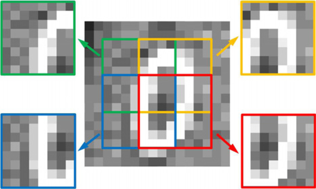
An image of size can be decomposed into many small image patches of size . Each image patch is identified by the position of its top-left pixel. The number of pixels between the top left pixels of adjacent image patches is the sliding distance. In figure 1, the image patch is 8 × 8, and the sliding distance is 4. Note that an image x can be expressed as a single vector and each pixel occupies a unique position in this vector, so the image patch xj with top-left pixel at the jth location is also uniquely determined. Assume the image vector x is of length N, then the image patch xj = Rjx ϵ ℝn is extracted from x by the matrix Rj: ℝN → ℝn.
Figure 1.
Illustration of image patches and the sliding distance. A central area of the image is covered by four 8 × 8 image patches with the sliding distance 4.
A dictionary is a matrix D : ℝn′ → ℝn (n′ ≫ n). A column of the dictionary is called an atom. In most cases, a dictionary is built from high-quality sample images of the same types of objects obtained from the same imaging modality (for example, using CT, MRI and photography). The dictionary and the image patch from a given image are connected by the so-called Sparse-Land model. The Sparse-Land model was first proposed for image denoising (Elad and Aharon 2006), then extended to other signal processing areas (Elad 2010). It suggests that an image patch xj can be built as a linear combination of a few atoms from the dictionary D, that is,
| (1) |
where aj is the sparse representation (SR) of patch xj under dictionary D, with few nonzero elements, and εj is a controllable error. Recall that the dictionary is built from high-quality images, so if the image patch in x is contaminated by missing pixels or noise, we can use the combination of the atoms from the dictionary to replace this image patch, hence improving the image quality. Such a process is called dictionary learning (DL).
2.2. DL-based image reconstruction
The heuristic of DL is that a group of pixels, instead of a single pixel, is the minimum unit in the process. With the idea of DL, the CT reconstruction problem can be stated as
| (2) |
where ‖x‖TV is the TV norm of an image x, ‖aj‖0 is the l0 norm of aj , ρ is the threshold of sparsity, M is a system matrix describing the forward projection, y is a measured dataset and εa is a small positive value representing the error threshold.
Mathematically, equation (2) contains the following three sub-problems, which can be solved in an alternating fashion.
Sub-problem A
| (3) |
This sub-problem is called atom matching. Given an image x, we want to find the sparsest representation aj with respect to the dictionary D, and the number of nonzero elements in aj is not larger than ρ. To solve this problem, the orthogonal matching pursuit (OMP) algorithm (Tropp 2004) can be used.
Sub-problem B
| (4) |
This is the well-known TV minimization problem subject to two constraints: non-negativity x ≥ 0 and data fidelity (Sidky et al 2006). We should emphasize here that the TV term is not part of the standard DL process. Actually it can be removed from equation (2) if we are only interested in the performance of DL. However, most of the images we are dealing with are relatively sparse (the gradient images of which have few nonzero elements), and the TV minimization has demonstrated its power for reconstructing those images. So the TV term here can help reduce image artifacts, hence reducing the probability of incorrect atom matching. On the other hand, if the images are not sparse or cannot be transformed to be sparse, we should not use the TV term for regularization.
Sub-problem C
| (5) |
This sub-problem aims at updating an image with respect to a fixed dictionary and an associated SR. The closed-form solution to this problem is as follows (Elad and Aharon 2006):
| (6) |
where the superscript T denotes the transpose operation of the matrix Rj, and is a matrix of size N × N, each of whose diagonal elements represents the number of ‘overlapped patches’ at a given position. Note that is a diagonal matrix, and its inverse can be done element-wise.
2.3. From one dictionary to dual dictionaries
DL-based image reconstruction in the few-view case has been studied in Xu et al (2011) and Liao and Sapiro (2008). In these studies, the K-singular value decomposition (K-SVD) algorithm (Aharon et al 2006) was employed to construct a global/adaptive dictionary, and then the DL step was incorporated in the iterative reconstruction procedure to update an intermediate image. These algorithms, either the global dictionary-based statistical iterative reconstruction (SIR) or the adaptive dictionary-based SIR, only used a single dictionary in the whole process. That is, in the atom matching step (sub-problem A) and the image updating step (sub-problem C), the symbol D points to the same dictionary. Inspired by their success, we are motivated to study whether the image quality can be further improved when more dictionaries are involved. In this section, we are investigating the possibility of using two dictionaries.
Let xt be a low-quality image reconstructed from few views, and xg be its high-quality counterpart from full views. They are connected by the observation model xt = Hxg + vt, where vt is the additive noise and H is the transform operator. In this context, H consists of two operations: forward projection and few-view reconstruction. Denoting the image patch extracted from , and inserting this formula into the observation model results in
| (7) |
Let , then equation (7) can be rewritten as
| (8) |
where the additive noise in this patch, and Lj is a local operator transforming the high-quality image patch into a low-quality image patch . On the other hand, the high-quality image patch can also be expressed as the linear combination of the atoms in the global dictionary DG, that is,
| (9) |
where aj is a vector of the coefficients and is the additive noise in this patch. Inserting equation (9) into equation (8) gives us
| (10) |
Equation (10) shows that if we want to recover a high-quality image patch from a low-quality image patch , the local operator Lj must be considered. Let DT = LjDG be a transitional dictionary, then equation (10) can be simplified as
| (11) |
in which the noise term is controllable. From equations (9) and (11) we find that a high-quality image patch and a low-quality image patch share the same representation under different dictionaries. This observation suggests a solution to our problem. That is, for a low-quality image patch, we should first find its coefficients under the transitional dictionary, and then multiply the coefficients by the global dictionary to recover the high-quality image patch. When all the low-quality patches in a few-view reconstructed image are replaced by the high-quality patches, the image quality is improved.
2.4. Construction of dual dictionaries
For any dictionary-based method to work, the construction of an excellent dictionary is most critical. In a broad sense, there are three ways to construct a dictionary: analytic, training-based, and direct. The analytic method constructs dictionaries based on mathematical tools, such as the Fourier transform, curvelet, contourlet, bandlet and wavelet transforms (Rubinstein et al 2010). The resultant dictionaries usually have the smallest sizes, and their implementation is efficient. However, the mathematical functions are nonspecific to model real-world images. To address this issue, the training-based method was proposed to be specific and adaptive. Unlike the analytic method, the training method focuses on real images. Assuming that images are sparse, the training method extracts structural elements in training images, and then a target image can be sparsely represented in these elements. In practice, the training method can be typically superior to the analytic method since it reflects the specific complexity of underlying structures which cannot be more sparsely described in generic mathematical functions. Research into developing and applying the training-based approach has been very popular recently. Typical training methods include the method of optimal directions (Engan et al 1999), generalized principal component analysis (Vidal et al 2005), and K-SVD (Aharon et al 2006). Compared to the aforementioned methods, the direct method is quite straightforward. It directly extracts image patches from sample images, and uses them or some of them to form a dictionary, without any transformation, decomposition or combination. The direct method preserves all details in the sample images, and a target image can be effectively recovered if the sample images are well chosen. This method is very popular in super-resolution imaging (Chang et al 2004, Yang et al 2008).
In this feasibility study, we use the direct method to construct the dictionaries. First, we need to prepare two sets of the sample images: one set of high-quality CT images (i.e. full-view, noise-free, etc) and one set of low-quality CT images (i.e. few-view, noisy, etc). For the problem of few-view reconstruction, if real projections are available, we can use full-view data to generate high-quality images and down-sampled data to generate low-quality images. If real data are not available, we use numerical methods (forward projection and then backprojection) to generate low-quality images.
Second, the image patches are extracted from the sample images and expressed as feature vectors. The feature vector is used to distinguish one image patch from others. The most common features are the pixel values. However, the pixel values alone cannot reflect the relationship of one pixel and its nearby pixels, so we may use first-order or second-order gradient distributions to enhance the feature vector. For low-quality image patches the features are defined as the pixel values and their first-order gradient vector along two directions. Hence, each pixel has three characteristic values. All this information will be recorded in a feature vector and then written into the transitional dictionary as an atom. For high-quality image patches, only the pixel values are recorded, since they can be directly linked to their counterparts in the transitional dictionary. For an image patch of size , the atom in the transitional dictionary has 3n features and in the global dictionary it has n features. The atoms in the two dictionaries are in one-to-one correspondence. To make full use of sample images, the extracted image patches can be rotated to generate new patches. Their mirror images can be included as well.
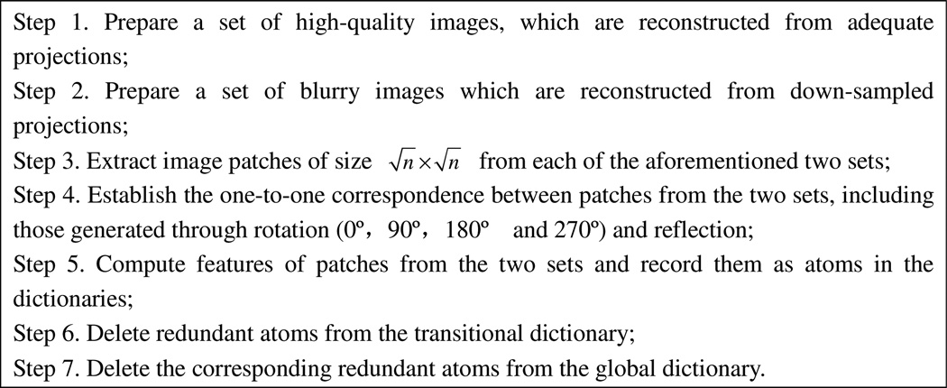
Even though we have used complicated features to describe the image patch, there still exist many atoms having similar feature representations; therefore, the last step is to reduce the redundancy of the dictionaries. This redundancy can be measured in terms of the Euclidean distance. For a given atom in the transitional dictionary and a pre-set threshold, those atoms whose Euclidean distances are less than the threshold will be removed from the transitional dictionary, and their counterparts will be removed from the global dictionary. To summarize, the steps for dictionary construction are illustrated in figure 2.
Figure 2.
Steps for dictionary construction.
2.5. SART–TV–DL algorithm
We have formulated the CT reconstruction problem with the idea of DL and discussed the strategy of dictionary construction, but it is still not clear to us how to solve the reconstruction problem via dual dictionaries. In this section we will give the implementation details of our SART–TV–DL algorithm.
The proposed algorithm consists of three components: SART reconstruction, TV minimization and DL. Both TV minimization and DL work as regularization terms; they cannot reconstruct the image directly from the projections. They must work together with one reconstruction algorithm, such as FBP, expectation maximization, maximum likelihood, SART, etc. In this study, we focus on SART (Andersen and Kak 1984) since it is widely used when dealing with few-view reconstruction problems. Notice that an image can be either presented as a matrix of size or a vector of length N, where N is the total number of pixels in the image. We may use the symbol x with one or two subscripts to describe these two forms. The imaging system is formulated as Mx = y, where M is a system matrix, and y is a measured dataset. We define
| (12) |
| (13) |
whereW is the length of y,which corresponds to the number of detector cells, and the subscripts m1 and m2 indicate the element locations.
Then the SART formula can be expressed as
| (14) |
where the superscript k is the iteration index and ky is the calculated data at the kth iteration.
TV minimization can be implemented by use of the gradient descent method (Sidky et al 2006). The magnitude of the gradient can be approximately expressed as
| (15) |
The image TV can be defined as ‖x‖TV = ΣiΣjτi,j. The steepest descent direction is then defined by
| (16) |
where ε is a small positive number in the denominator for the consideration of avoiding any singularity. In summary, the formula for TV minimization is
| (17) |
where β is the length of each gradient-descent step and q is the iteration index. The result of the SART algorithm at the kth iteration is used as an initial image for TV minimization, and Δx = ‖k+1x – kx‖ is the difference between the results of the SART algorithm at the kth and the (k–1)th iterations.
As mentioned in section 2.2, the DL process consists of two parts: atom matching and image updating. In the atom matching part, we need to find the SR for each patch in the target image. Since our dictionary is relatively large, it is not practical to search the whole dictionary for the SR. Thus, a practical solution can be obtained in two steps.
(a) Calculate the Euclidean distances from the current patch to each of the atoms in the transitional dictionary and find a set of atoms (which have the shortest Euclidean distances) to form a local transitional dictionary , and a local dictionary of DG is determined accordingly.
(b) Use the OMP algorithm to find a local SR wj that minimizes the local reconstruction error
| (18) |
The OMP algorithm stops when or the maximum iteration number for OMP is reached, where εb is a small positive value.
In the image updating part, the SR wj in terms of the local dictionary is used for updating an image patch , and then the updated image patches are recorded in a matrix. They are not written back to the target image until all image patches have been updated and recorded. Finally, the image x can be updated as
| (19) |
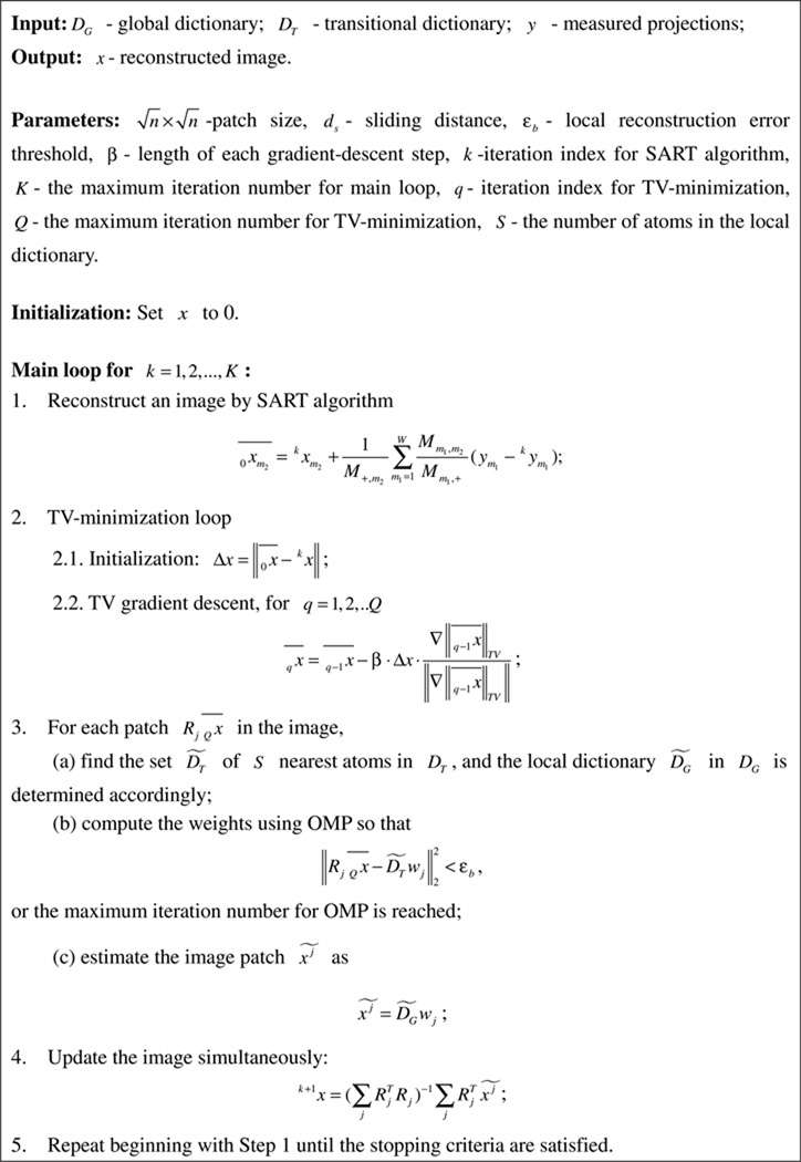
The workflow for the SART–TV–DL algorithm is summarized in figure 3.
Figure 3.
Workflow for SART–TV–DL reconstruction. is a vector representing the result of the SART algorithm at the kth iteration, and is the m2th element of .
3. Numerical and experimental results
In this section, we will report four experiments to evaluate and validate the proposed algorithm. The first two experiments used true CT images and simulated projections, in which we are interested in the performance of our algorithm under ideal conditions. The third and fourth experiments used real data collected using the Shanghai Synchrotron Radiation Facility. Reconstructions were quantitatively evaluated in terms of the root mean square error (RMSE) with respect to different patch sizes and sliding distances.
3.1. Simulated data without noise
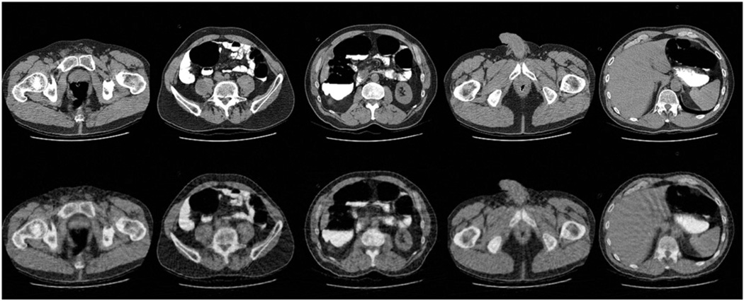
The first experiment was performed under ideal conditions. That is, projections were generated numerically without any noise purposely added. For construction of a global dictionary, we used five typical cross-section CT slices of the human body as a sample set. All images were downloaded from NCIA (National Cancer Imaging Archive, http://ncia.nci.nih.gov). The sample images and the reconstructed images were 256 × 256 pixels, see figure 4. From each image 20 000 patches were randomly extracted. The patches were 6 × 6 with the sliding distance of 2 pixels.
Figure 4.
Sample set of clinical CT images. First row: true CT slices. Second row: the images reconstructed from 50 views using the SART algorithm.
To construct a transitional dictionary, we synthesized projection data from these CT slices, and then reconstructed them using the SART algorithm in few-view settings. In the simulation, 50 and 30 views were uniformly distributed over 360°. The resultant images were used to generate patches of the transitional dictionary. The patches in the global dictionary were linked to that in the transitional dictionary via a one-to-one mapping.
DL-based reconstruction was started from the top left of an original image and ended at the bottom right. In the process, all Euclidean distances were calculated between a given image patch and the atoms in the transitional dictionary DT·S = 10 nearest atoms in DT were used to approximate the image patch using OMP. In the implementation of OMP, at most ρ = 4 atoms were used. The local reconstruction error threshold εb was set to 0.001. Once the coefficients were determined, the involved atoms in DT would be replaced by their counterparts in DG to update the image patch. The updated patch was recorded in another matrix as an intermediate result. It was written back to the original image simultaneously when all patches were updated.
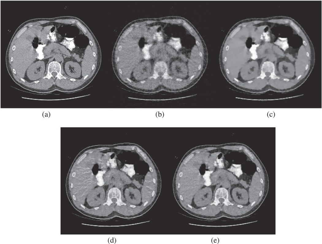
Our proposed DL-based reconstruction method significantly improved the image quality while the SART algorithm only slightly changed the image over one iteration. It was not necessary that the DL process be immediately executed after the SART step in each iteration; instead, it was performed after every 30 iterations and still yielded good results. A SART iteration here is a full iteration, where all views are backprojected. The reconstruction process was stopped after 125 iterations, which meant that the SART–TV algorithm was executed 125 times and the DL process was executed only 4 times.
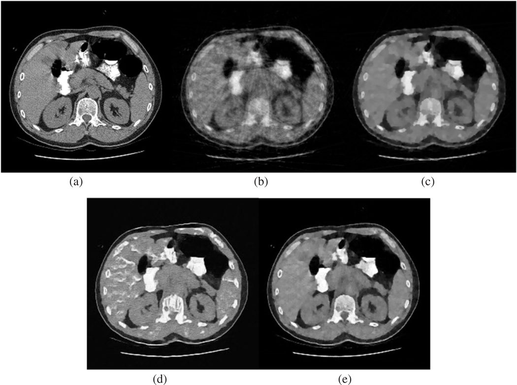
The effects of TV and DL regularizations are presented in figures 5 and 6. The gradient-descent step was fixed at 0.06 for the case of 50 views and 0.08 for the case of 30 views, and the number of TV-steepest descent iterations was set to 2. Clearly, the artifacts caused by incorrect atom matching were substantially suppressed by the use of the TV term.
Figure 5.
Few-view reconstructions from 50 noiseless projections over 360°. (a) The true image, (b) the result obtained using the SART algorithm, (c) the SART–TV algorithm, (d) the SART–DL algorithm, and (e) the SART–TV–DL algorithm.
Figure 6.
Few-view reconstructions from 30 noiseless projections over 360°. (a) The true image, (b) the result obtained using the SART algorithm, (c) the SART–TV algorithm, (d) the SART–DL algorithm, and (e) the SART–TV–DL algorithm.
3.2. Simulated data with noise
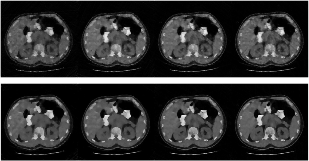
The second experiment was performed using noisy data. For the case of reconstruction from 30 projections, Gaussian noise of 27.5, 32.5, 37.5 and 42.5 dB (signal-to-noise ratio) were added to the sinograms. The dictionaries and the parameters were the same as those in the first experiment. The results are displayed in figure 7. It was evident that our algorithm showed strong robustness against noise.
Figure 7.
Few-view reconstruction from 30 noisy projections over 360°. The first row shows the reconstructions using the SART–TV algorithm at noise levels 27.5, 32.5, 37.5, and 42.5 dB. The second row shows the results by the proposed algorithm.
3.3. Real data
In the third experiment, we used real data collected using the Shanghai Synchrotron Radiation Facility. The detector array consisted of 805 bins covering a length of 35 mm. A total of 1150 projections were acquired over 180°. Unless otherwise specified, reconstructed images were of 512 × 512 pixels.
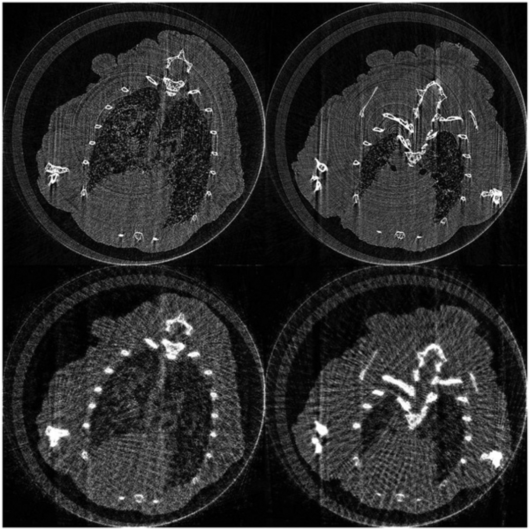
Two images reconstructed from 575 projections were used as sample images for the global dictionary. The projections were then down-sampled to 46, about one-twelfth of the original dataset. Due to the data incompleteness, the reconstructed images suffered from severe artifacts. They were used to construct the transition dictionary, see figure 8. With the patch sizes of 9 × 9, 17 × 17, and 36 × 36 and a sliding distance of 3 pixels, 40 000 image patches were randomly extracted from each image.
Figure 8.
Sample images in the third experiment. Images in the first and second rows are for the global and transitional dictionaries, respectively.
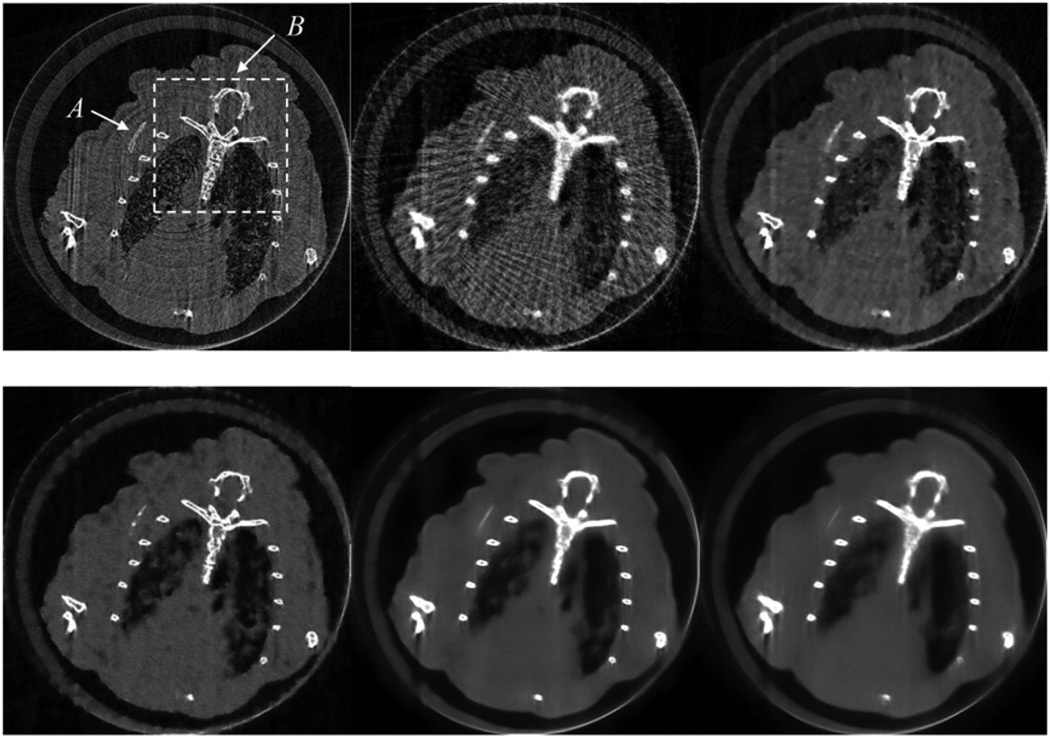
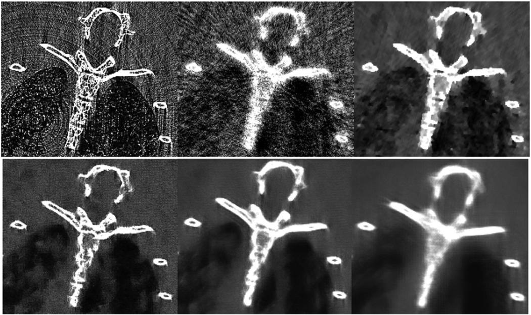
The DL process was performed after every 10 iterations. The total number of iterations was fixed at 40. The reconstructed images are displayed in figure 9.We paid special attention to two bony structures, A and B, in the images, as indicated by the arrow and the square. The zoomed-in versions of B are shown in figure 10. We found that the thin bone A was reconstructed as a collection of disconnected dots in the case of patch size 9 × 9. This could be explained as follows: due to the down-sample projections, the thin bone A was not well reconstructed. Two sets of pixels in this structure were much brighter than their nearby pixels. This phenomenon also occurred in the results obtained using the SART or SART–TV algorithm. It was noted that the patch size of 9 × 9 was a small patch; hence these two sets of pixels would make major contributions to the image patches containing them. In other words, they became the major features of those image patches. During the DL process, the major features would be enhanced and the minor features (those with little contribution to the feature vector) would be suppressed. The final result, as we see, was disconnected dots. However, if we increase the size of the image patch, the contributions of these two sets of pixels to the feature vector would decrease considerably; then we could still reconstruct bone A as a continuous object; see the result of patch size 17 × 17 in figure 9.
Figure 9.
Top row: from left to right are the results obtained using SART from 575 projections, SART from 46 projections and SART–TV from 46 projections. Bottom row: from left to right are the results obtained using the proposed method from 46 projections with patch sizes 9 × 9, 17 × 17, and 36 × 36.
Figure 10.
Zoomed-in views of a ROI B shown in figure 9.
Now let us look at bone B. It was much more complicated than bone A. Clearly, the result of patch size 9 × 9 was better than others, see figure 10. When we increased the size of image patch, the reconstructed images became blurry. This was easy to understand. A large image patch has numerous features. Thus the dictionary should be relatively large, or we cannot find the most suitable atoms to approximate the given image patch.
In summary, for a dictionary of limited size, reconstructions with small patch size usually have better performance; if the dictionary can be relatively large, reconstructions with large patch size may provide more reliable results.
3.4. Parameter optimization
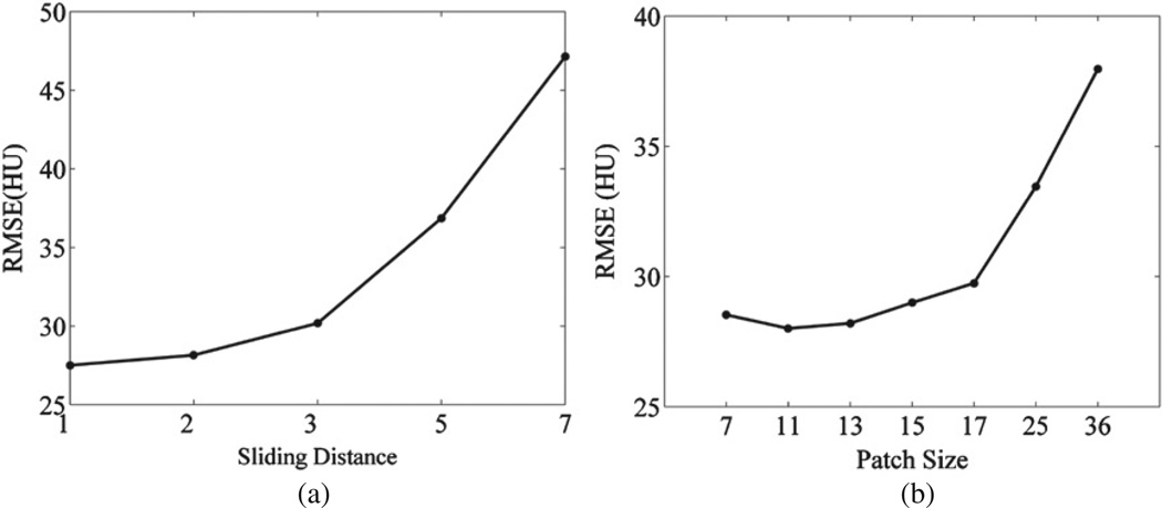
The last experiment was designed to evaluate the effects of sliding distance and patch size when the dictionaries were fixed. Fixing the patch size at 9 × 9, reconstructions were performed when the sliding distance was increased from 1 to 7. Then, fixing the sliding distance at 3, the reconstructions were performed for the patch size from 7 × 7 to 36 × 36. Keeping other parameters intact as in the third experiment, the performances were evaluated in terms of RMSE, that is,
| (20) |
where and ηj are the reconstructed and true values at the jth pixel, respectively, and J is the number of pixels. The results are shown in figure 11. It is observed that for a fixed patch size, the shorter the sliding distance, the better the performance is (figure 11(a)). On the other hand, if the sliding distance was fixed, the image quality became worse when the patch size was increased (figure 11(b)). This trend was more evident when the patch size was larger than 17 × 17. Hence, it is suggested to use a patch size less than 17 × 17 and a sliding distance less than 3 for an image of 512 × 512 pixels.
Figure 11.
Parameter optimization with respect to (a) the sliding distance and (b) the patch size.
4. Discussions and conclusion
The history of DL can be traced back to jigsaw puzzles. A Chinese jigsaw puzzle called a ‘tangram’ has only seven pieces, but using the human imagination those pieces can form thousands of shapes, and this number is ever-growing. Over the past few years, the DL-based methods have attracted increasing attention and claimed significant successes in almost every area of image and signal processing (Elad 2010).
The essence of our proposed algorithm is the use of dual dictionaries: one transitional dictionary for atom matching and one global dictionary for image updating. This idea was developed for super-resolution imaging, which uses two dictionaries to link low-resolution sample images and high-resolution sample images. The novelty of the work lies in the extension of the dual DL approach for few-view reconstruction.
The performance of the DL-based reconstruction depends heavily on the relevance of the dictionaries and the target object. In our experiments, the sample images and the raw images or data were assumed from the same CT scanner (but from different patients), the image quality was consistent, and the image patches could be directly extracted to construct the dictionaries. Using this method, the dictionaries contain almost all significant details in the sample images. However, a major drawback is that the dictionaries so constructed are much larger than those constructed using other methods.
In the case of 2D reconstruction, the computational complexity of the DL process is O(n2) and of the SART–TV algorithm is O(n3). As mentioned in section 3.1, the DL process was not performed after each SART–TV iteration, so their computational complexity should be separately analyzed. Although the DL process has less computational complexity than the SART–TV algorithm, it consumes more time under the aforementioned experimental conditions. This is because the time cost of the SART–TV algorithm depends on the maximum iterations (usually < 200), views (< 50) and detector cells (< 1000), while that of the DL technique depends on the size of dictionary (> 20 000) and the image patches in the reconstructed image (> 20 000). In the DL process, the atom matching step is most computationally expensive. For each image patch, we have to search the entire dictionary, calculate the Euclidean distances and then determine the S nearest atoms. Suppose the dictionary has N1 atoms, the reconstructed image is of N2 × N2 pixels; then with the sliding distance N3 and patch size N4 × N4, the core step in the atom matching will be executed times. Clearly, with a large sliding distance the time cost of the atom matching step will be greatly reduced. The size of the image patch will affect the computational complexity, but it has much less impact than the sliding distance. In the case of 3D reconstruction, i.e. cone-beam CT, the computational complexity of the DL process increases to O(n3) and that of the SART–TV algorithm is O(n4). Since we are doing 3D reconstructions, the concept of image patch could be extended to image block, which is a small volume of the 3D object. Suppose the dictionary has N1 atoms and the reconstructed volume is of N2 × N2 × N2 pixels, with sliding distance N3 and block size N4 × N4 × N4, the core step in the atom matching will be executed times. This is really computationally expensive for normal computers. As our next step, we are implementing the K-SVD and l1-DL algorithms to train dual dictionaries of limited size (Yang et al 2010, Fadili et al 2010) in the hope that satisfactory few-view reconstructions would also be achieved with more efficient dual dictionaries.
In conclusion, we have proposed a novel SART–TV–DL algorithm for few-view reconstruction. This algorithm has been evaluated in numerical simulation and with real CT datasets. Our preliminary results have demonstrated the potential of impressive image reconstruction from only 30–50 views in realistic scenarios. This approach seems promising for several preclinical and clinical applications such as image-guided radiotherapy, C-arm cardiac imaging, breast CT and tomosynthesis, and stationary multi-source CT, as well as nondestructive evaluation and security screening.
Acknowledgments
This work was supported in part by the National Basic Research Program of China (2010CB834302), the National Science Foundation of China (30570511 and 30770589), the National High Technology Research and Development Program of China (2007AA02Z452), and the National Science Foundation of USA (NSF/CMMI0923297) and the National Institute of Health (NIBIB R01 EB011785).
Contributor Information
Yang Lu, Email: lvyang@sjtu.edu.cn.
Jun Zhao, Email: junzhao@sjtu.edu.cn.
Ge Wang, Email: wangg@vt.edu.
References
- Aharon M, Elad M, Bruckstein A. K-SVD: an algorithm for designing overcomplete dictionaries for sparse representation. IEEE Trans. Signal Process. 2006;54:4311–4322. [Google Scholar]
- Andersen A, Kak A. Simultaneous algebraic reconstruction technique (SART): a superior implementation of the ART algorithm. Ultrason. Imaging. 1984;6:81–94. doi: 10.1177/016173468400600107. [DOI] [PubMed] [Google Scholar]
- Chang H, Yeung DY, Xiong Y. Super-resolution through neighbor embedding. Computer Vision and Pattern Recognition; Proc. IEEE Comput. Soc. Conf.; 27 June–2 July 2004; 2004. pp. 275–282. [Google Scholar]
- Chen GH, Tang J, Leng S. Prior image constrained compressed sensing (PICCS): a method to accurately reconstruct dynamic CT images from highly undersampled projection data sets. Med. Phys. 2008;35:660. doi: 10.1118/1.2836423. [DOI] [PMC free article] [PubMed] [Google Scholar]
- Donoho DL. Compressed sensing. IEEE Trans. Inf. Theory. 2006;52:1289–1306. [Google Scholar]
- Elad M. Sparse and Redundant Representations: From Theory to Applications in Signal and Image Processing. Berlin: Springer; 2010. [Google Scholar]
- Elad M, Aharon M. Image denoising via sparse and redundant representations over learned dictionaries. IEEE Trans. Image Process. 2006;15:3736–3745. doi: 10.1109/tip.2006.881969. [DOI] [PubMed] [Google Scholar]
- Engan K, Aase SO, Husoy H. Method of optimal directions for frame design. Acoustics, Speech and Signal Processing; Proc. IEEE Int. Conf; 1999. pp. 2443–2446. [Google Scholar]
- Fadili MJ, Starck JL, Bobin J, Moudden Y. Image decomposition and separation using sparse representations: an overview. Proc. IEEE. 2010;98:983–994. [Google Scholar]
- Gordon R, Bender R, Herman GT. Algebraic reconstruction techniques (ART) for three-dimensional electron microscopy and X-ray photography. J. Theor. Biol. 1970;29:471–481. doi: 10.1016/0022-5193(70)90109-8. [DOI] [PubMed] [Google Scholar]
- Liao HY, Sapiro G. Sparse representations for limited data tomography. 5th IEEE Int. Symp. on Biomedical Imaging: From Nano to Macro (ISBI 2008). (14–17 May 2008) 2008:1375–1378. [Google Scholar]
- Natterer F. The Mathematics of Computerized Tomography. Philadelphia, PA: Society for Industrial Mathematics; 2001. [Google Scholar]
- Ravishankar S, Bresler Y. MR image reconstruction from highly undersampled k-space data by dictionary learning. IEEE Trans. Med. Imaging. 2011;30:1028–1041. doi: 10.1109/TMI.2010.2090538. [DOI] [PubMed] [Google Scholar]
- Rubinstein R, Bruckstein AM, Elad M. Dictionaries for sparse representation modeling. Proc. IEEE. 2010;98:1045–1057. [Google Scholar]
- Shen B, Hu W, Zhang Y, Zhang YJ. Image inpainting via sparse representation. Acoustics, Speech and Signal Processing (ICASSP 2009) 2009:697–700. [Google Scholar]
- Sidky EY, Kao CM, Pan X. Accurate image reconstruction from few-views and limited-angle data in divergent-beam CT. J. X-Ray Sci. Technol. 2006;14:119–139. [Google Scholar]
- Tropp JA. Greed is good: algorithmic results for sparse approximation. IEEE Trans. Inf. Theory. 2004;50:2231–2242. [Google Scholar]
- Vidal R, Ma Y, Sastry S. Generalized principal component analysis (GPCA) IEEE Trans. Pattern Anal. Mach. Intell. 2005;27:1945–1959. doi: 10.1109/TPAMI.2005.244. [DOI] [PubMed] [Google Scholar]
- Xu Q, Yu H, Mou X, Wang G. Dictionary learning based low-dose x-ray CT reconstruction; 11th Int. Meeting on Fully Three-Dimensional Image Reconstruction in Radiology and Nuclear Medicine; Potsdam, Germany. 2011. pp. 258–261. [Google Scholar]
- Yang J, Wright J, Huang T, Ma Y. Computer Vision and Pattern Recognition (IEEE Conf.) 2008. Image super-resolution as sparse representation of raw image patches; pp. 1–8. [Google Scholar]
- Yang J, Wright J, Huang TS, Ma Y. Image super-resolution via sparse representation. IEEE Trans. Image Process. 2010;19:2861–2873. doi: 10.1109/TIP.2010.2050625. [DOI] [PubMed] [Google Scholar]
- Ye Y, Yu H, Wei Y, Wang G. A general local reconstruction approach based on a truncated Hilbert transform. Int J. Biomed. Imaging. 2007:63634. doi: 10.1155/2007/63634. 2007. [DOI] [PMC free article] [PubMed] [Google Scholar]
- Yu H, Wang G. SART-type image reconstruction from a limited number of projections with the sparsity constraint. J. Biomed. Imaging. 2010a:934847. doi: 10.1155/2010/934847. 2010. [DOI] [PMC free article] [PubMed] [Google Scholar]
- Yu H, Wang G. A soft-threshold filtering approach for reconstruction from a limited number of projections. Phys. Med. Biol. 2010b;55:3905. doi: 10.1088/0031-9155/55/13/022. [DOI] [PMC free article] [PubMed] [Google Scholar]


