Probabilistic Clustering and Quantitative Analysis of White Matter Fiber Tracts

Abstract

A novel framework for joint clustering and point-by-point mapping of white matter fiber pathways is presented. Accurate clustering of the trajectories into fiber bundles requires point correspondence along the fiber pathways determined. This knowledge is also crucial for any tract-oriented quantitative analysis. We employ an expectation-maximization (EM) algorithm to cluster the trajectories in a Gamma mixture model context. The result of clustering is the probabilistic assignment of the fiber trajectories to each cluster, an estimate of the cluster parameters, and point correspondences. Point-by-point correspondence of the trajectories within a bundle is obtained by constructing a distance map and a label map from each cluster center at every iteration of the EM algorithm. This offers a time-efficient alternative to pairwise curve matching of all trajectories with respect to each cluster center. Probabilistic assignment of the trajectories to clusters is controlled by imposing a minimum threshold on the membership probabilities, to remove outliers in a principled way. The presented results confirm the efficiency and effectiveness of the proposed framework for quantitative analysis of diffusion tensor MRI.

1 Introduction

In recent years, a significant amount of work has been devoted to extracting information from diffusion tensor images to study brain changes related to development, aging, and different pathologies. Developing tools to perform accurate and comprehensive quantitative analysis is thus of great interest [1]. However, most clinical studies performed to date are limited to the analysis of local parameters, such as fractional anisotropy, measured in a manually defined region of interest (ROI) and averaged over groups of healthy and patient cases. Such methods are sensitive to the accuracy of specifying the ROIs and are prone to user errors. Others have performed a voxel-based analysis of a registered DTI dataset, which requires non-linear warping of the tensor field [2], which in turn needs re-orientation of the tensors [3, 4].

An alternative approach is to compute the quantitative parameters of interest along the trajectories [1, 5] which makes more sense as the underlying anatomical unit in DT images is a fiber tract, not a voxel. Such analysis is valuable especially if performed on a group of trajectories that correspond to an anatomical bundle of a fiber tract. This way, statistical parameters, such as mean and standard deviation, can be calculated, making inter-subject comparisons possible. To accomplish this goal, algorithms are required to segment the trajectories into bundles and to obtain correspondence between points on trajectories within a bundle.

Several papers have addressed the issue of grouping the trajectories into bundles [6–8] but without going further into quantitative analysis. The outcome of these methods is a set of labeled trajectories, each assigned to a cluster. Point-by-point correspondence between the trajectories of each cluster, however, is not determined rigorously. In one of the early works on DT-MRI analysis, Ding et al. [9] tackled the issue of quantification of tracts by finding the corresponding segments, which they defined as the portion of a trajectory that has point-wise correspondence to a portion of another trajectory. They assumed that the seed points of two trajectories to be compared correspond to each other, which is not the case unless all trajectories are seeded from a small ROI. The algorithm is thus inadequate for whole brain fiber analysis. Batchelor et al. [10] proposed different tools to quantify the shape of fiber tracts. They noted the problem of point correspondence but made the assumption that it is approximately achieved by proper choice of the seed point and regularly sampling the arc-length. With point correspondence roughly known, they applied the Procrustes algorithm to register the trajectories. There is also a series of work by Gerig et al. (see for example [1]), which described methods and applications for tract-oriented quantitative analysis. They dealt with the issue of correspondence by letting the user define a common origin for the set of trajectories in each cluster based on geometric criteria or based on anatomical landmarks. In their latest work [11], they also proposed the Procrustes algorithm for the registration of the trajectories to compute the average tensor. Although these methods provide some valuable information about the fibers, they suffer from a number of issues. They need manual setting of the common start points for all the trajectories in a cluster. Also, they assume the trajectories in a cluster have the same length, which is a reasonable assumption only if a small ROI is considered as the tractography seed points and the tractography algorithm gives full-length trajectories. Otherwise a thorough preprocessing is required. In our earlier work [12], we used a string matching algorithm to align all extracted trajectories with each cluster center at each iteration of our expectation-maximization (EM) clustering. The accuracy of this approach was limited by the simple curve matching algorithm used. More sophisticated three-dimensional (3-D) curve matching methods could be performed but at the expense of increased computational effort [10].

This paper presents a clustering method that aims to facilitate quantitative analysis as the next step in the study of DT images. A statistical model of the fiber bundles is calculated as the mean and standard deviation of a parametric representation of the trajectories. Using this model representation, expectation-maximization (EM) is performed to cluster the trajectories in a mixture model framework. We obtain correspondence between points on trajectories within a bundle by building distance maps for each cluster center. The proposed method can potentially benefit from an atlas for the initialization step and as the prior map in the EM algorithm. All these tasks are done in a unified framework and the results are soft assignment of trajectories to labels and the point-by-point correspondence to each cluster center.

2 Similarity measure

Determining the point correspondence between a pair of trajectories is not trivial [9, 7] but if achieved, it not only makes the computation of their similarity, needed for clustering, straightforward but also makes it possible to measure the quantitative parameters within a bundle. Although many authors acknowledge that point-by-point correspondence of the trajectories should be defined by a curve matching algorithm for accurate clustering and quantitative analysis [1, 10, 9], to our knowledge this problem has not been solved to date. The difficulty lies in the fact that the number of trajectories is usually very large, especially when tractography is performed on the whole brain. This makes it computationally very inefficient, if not impossible, to perform a rigorous curve matching algorithm on every pair of trajectories. Here, we propose a novel approach for measuring the similarity of 3-D curves in a large dataset that includes the whole information of the curve for more accurate clustering and further quantitative analysis.

We treat each trajectory as a 3-D curve, i.e., an ordered set of points, r_i = {r_ij}. The set of trajectories is clustered to a number of subsets by assigning a membership probability p_ik to each trajectory, r_i, to denote its membership in the kth cluster (∀i, Σ_k p_ik = 1). For each cluster, a 3-D curve, μ_k = {μ_kj}, is defined as the cluster center where each point, μ_kj, is obtained as the average of all of its corresponding points on the trajectories:

$${\mathit{\mu }}_k={\displaystyle \sum _i}{p}_{\mathit{\text{ik}}}{\mathbf{r}}_i^{(k)},$$ (1)

where ${\mathbf{r}}_i^{(k)}$ is the trajectory r_i, re-parametrized to have point correspondence to cluster k, and the summation is performed over all trajectories. h

Our space includes a set of 3-D curves and a number of cluster centers. From each center, μ_k, we construct an Euclidean distance map:

$${𝒟}_k(\mathbf{x})=\underset{j}{\text{min }}d(\mathbf{x},{\mathit{\mu }}_{\mathit{\text{kj}}})$$ (2)

and the nearest-neighbor transform, ℒ_k:

$${ℒ}_k(\mathbf{x})=\text{arg}\underset{j}{\text{ min }}d(\mathbf{x},{\mathit{\mu }}_{\mathit{\text{kj}}})$$ (3)

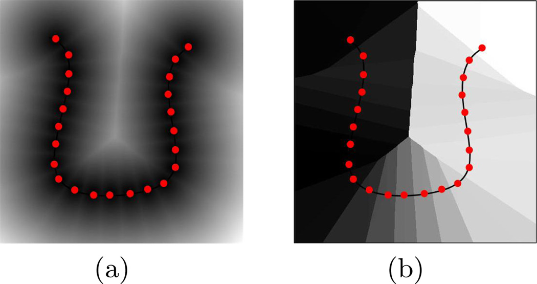
where d(x, μ_kj) is the Euclidean distance from the point x in the space to the jth point on the kth center. Each element of ℒ_k will thus contain the linear index of the nearest point of the center μ_k. Fig. 1 shows the distance map and label map constructed from a sample 2-D curve The label map partitions the space into regions that each correspond to a point of the center. Now, for every curve, r_i = {r_ij} in the space, the distance to the center μ_k can be measured simply as:

$$d_E({\mathbf{r}}_i,{\mathit{\mu }}_k)={\displaystyle \sum _j}{𝒟}_k({\mathbf{r}}_{\mathit{\text{ij}}}),$$ (4)

and by projecting it onto the label map, its point correspondence to the center is readily achieved.

Fig. 1.

(a) Distance map from sample points on a cluster center and (b) the point correspondence label map with the center overlaid. Each region in the label map, displayed by a different color, consists of all of the points in the space that have the minimum distance to a specific point on the cluster center. Therefore, projecting any curve onto this label map determines the point correspondence of each of its samples to the center based on which region that sample is located.

A spatial distance by itself does not encode enough information for measuring the pair-wise similarity. One obvious issue is the variable lengths of the trajectories. Another issue is whether the trajectory has one-to-one point correspondence to the cluster center, which is the case when they are similar in shape. Thus, any repeated or missing match represents shape dissimilarity. A penalty is therefore added if there are multiple points on the trajectory that correspond to a single point on the cluster center. We add the penalty term, d_penalty to the Euclidean distance and normalize to the length of the fiber trajectory, L_i, to obtain the adjusted distance, d_a(r_i, μ_k):

$$d_{\mathit{\text{ik}}}=d_a({\mathbf{r}}_i,{\mathit{\mu }}_k)=\frac{d_E({\mathbf{r}}_i,{\mathit{\mu }}_k)+d_{\text{penalty}}({\mathbf{r}}_i,{\mathit{\mu }}_k)}{L_i}.$$ (5)

3 Mixture Model

In the previous section, we mapped our variable-length 3-D curves to a distance matrix, d_a = {d_ik}_{N × K} where N is the number of curves and K is the number of clusters. Note that d_ik’s depend on the cluster centers, μ_k’s, which evolve during the EM algorithm as will be discussed in the next section. In other words, the trajectories are mapped to the distance space through the cluster centers. The goal of this section is to estimate the likelihood membership of each curve to each cluster based on the values of the d_ik’s.

In mixture-model clustering, the data set is modeled by a finite number of density functions, where each cluster is represented by a parametric distribution. A common choice for the density functions of the data points, d_ik’s here, is the Gaussian distribution. However, a Gaussian distribution does not accurately represent the nature of the 3-D distance of the trajectories from the cluster centers. In the simplest form, the number of possible trajectories with a given distance from the center grows linearly with the distance, while the probability that they belong to that cluster decays exponentially. Among the well-known distributions, the Gamma distribution well models this combined trend. Furthermore, this distribution belongs to the exponential family of distribution functions for which the convergence of the EM algorithm is guaranteed. Given that the d_ik’s are non-negative, we assume that distance metrics for each cluster follow a Gamma distribution with parameter α_k and β_k:

$$\text{Gamma}(d|{\alpha }_k,{\beta }_k)=d^{{\alpha }_k-1}\frac{{\beta }_k^{{\alpha }_k}{e}^{-{\beta }_{k}d}}{\Gamma ({\alpha }_k)}\text{for }d\in [0,\mathrm{\infty })$$ (6)

where Г(.) is the gamma function. The mixture model then takes the following form:

$$p({\mathbf{r}}_i|\Theta )=p({\mathbf{d}}_i|\{{\theta }_k,w_k\})={\displaystyle \sum _k}{w}_k\text{Gamma}({\mathrm{d}}_{\text{ik}}|{\theta }_{\mathrm{k}}),$$ (7)

where r_i represents a trajectory which is mapped to a vector of distance metrics, d_i = [d_i1 …d_ik] as described in the previous section, w_k’s are mixing weights, and Θ is the collection of cluster parameters, θ_k = {α_k, β_k}, and the mapping parameter, μ_k. The goal is to infer Θ from a set of data points, r_i’s, assumed to be samples of distributions with density given by Equ. 7:

$$\widehat{\Theta }=\text{arg}\underset{\Theta }{\text{ max}}\{\text{log }p(\mathbf{r}|\Theta )\}$$ (8)

which gives a maximum likelihood (ML) estimation of the parameters. Since this estimation cannot be found analytically, the usual approach is to incorporate the Expectation-Maximization (EM) approach, which finds the local maximum of the likelihood function. Details are presented in the next section.

Cluster “no-match” (Outliers)

In mixture-model clustering, it is assumed that each data point is modeled by the mixture of a finite number of density components. However, in our case, there might be trajectories generated by the tractography that do not resemble any of the user- or atlas-initialized cluster centers or are not valid at all due to errors in the tractography stage. One way to deal with this issue is to allow the variance of densities to increase to accommodate these data. This would result in producing very spread bundles or even instability of the algorithm. A more practical alternative is to set a threshold so that if the membership likelihood of each trajectory in all clusters were less than that value, that trajectory would be removed from the processing data. In fact, with this threshold, the heterogeneity of the trajectories within each cluster is controlled. The larger the threshold is, the more compact are the resulting bundles, and consequently the greater is the number of unclustered trajectories. Handling outliers in such a principled way is not straightforward in previously proposed clustering schemes [7, 8, 12]. Unlike those methods, we allow the distribution of each cluster to have a different set of parameters (α_k’s, β_k’s), all inferred from the data by using the EM algorithm, and hence the user needs to set only the mentioned threshold to effectively remove the outliers.

4 Expectation Maximization Clustering

The EM algorithm produces a sequence of estimates of the parameters, Θ, and the hidden data, p_ik’s, in two consecutive steps:

Membership assignments(E-Step)

Assuming that the parameters of the clusters are known, the probability that the trajectory r_i belongs to cluster k is

$$p_{\mathit{\text{ik}}}=\text{Pr}(k|{\mathbf{r}}_i,\Theta )=\frac{w_{k}p({\mathbf{r}}_i|{\theta }_k)}{{\displaystyle {\sum }_k}{w}_{k}p({\mathbf{r}}_i|{\theta }_k)},$$ (9)

where p(r_i|θ_k) = Gamma(d_i|α_k, β_k).

Updating model parameters(M-Step)

The updated mixing weights are calculated as

$$w_k=\frac{1}{N}{\displaystyle \sum _{i=1}^N}{p}_{\mathit{\text{ik}}}.$$ (10)

Unlike the Gaussian mixture model, there is no closed form to update the ML estimate of shape parameter of the Gamma distribution. A good approximation can be made as [13]:

$${\alpha }_k\approx \frac{3-x+\sqrt{{(x-3)}^2+24x}}{12x},$$ (11)

where

$$x=\text{log }\left(\frac{{\displaystyle {\sum }_i}{p}_{\mathit{\text{ik}}}{d}_{\mathit{\text{ik}}}}{{\displaystyle {\sum }_i}{p}_{\mathit{\text{ik}}}}\right)-\frac{{\displaystyle {\sum }_i}{p}_{\mathit{\text{ik}}}\text{ log}(d_{\mathit{\text{ik}}})}{{\displaystyle {\sum }_i}{p}_{\mathit{\text{ik}}}}.$$ (12)

The ML estimate of the scale parameter is then updated by:

$${\beta }_k={\alpha }_k{\displaystyle \sum _i}{p}_{\mathit{\text{ik}}}/{\displaystyle \sum _i}{p}_{\mathit{\text{ik}}}{d}_{\mathit{\text{ik}}}.$$ (13)

With the point-by-point correspondence between each trajectory and the centers of clusters determined, the mapping parameter for each cluster is readily updated as:

$${\mathit{\mu }}_k=\frac{{\displaystyle {\sum }_i}{p}_{\mathit{\text{ik}}}{\mathbf{r}}_i^{(k)}}{{\displaystyle {\sum }_i}{p}_{\mathit{\text{ik}}}}$$ (14)

Initialization

We set the shape parameter of the Gamma distribution equal to one to have an exponential distribution which favors those trajectories most similar to the initial center. The scale parameter is then initialized to the mean values of data points of each cluster. The centers of clusters can be initialized manually by selecting a set of trajectories with different shapes from the data. Dependency of the algorithm on the initial centers will be discussed in Section 5. As an alternative, the initial cluster centers can be supplied by an atlas of fiber tracts, if available, such that the mean trajectories of the atlas clusters are employed after registering of the case to the atlas.

5 Results and Discussion

We applied our method on 3T DT-MR images with a spatial resolution of 1.054×1.054×2 mm, acquired from healthy volunteers. The streamline tractography [14] was used to reconstruct the trajectories from 3-D diffusion tensor data. The stopping criteria was reaching a point with fractional anisotropy (FA) less than 0.15 or a change of direction greater than 45°. As a three-dimensional curve, we represent each trajectory with an equally-spaced sequence of points. In our implementation, the distance between the successive samples is 5 mm, so the number of samples are different for each trajectory.

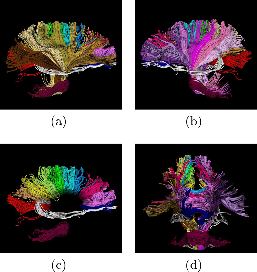
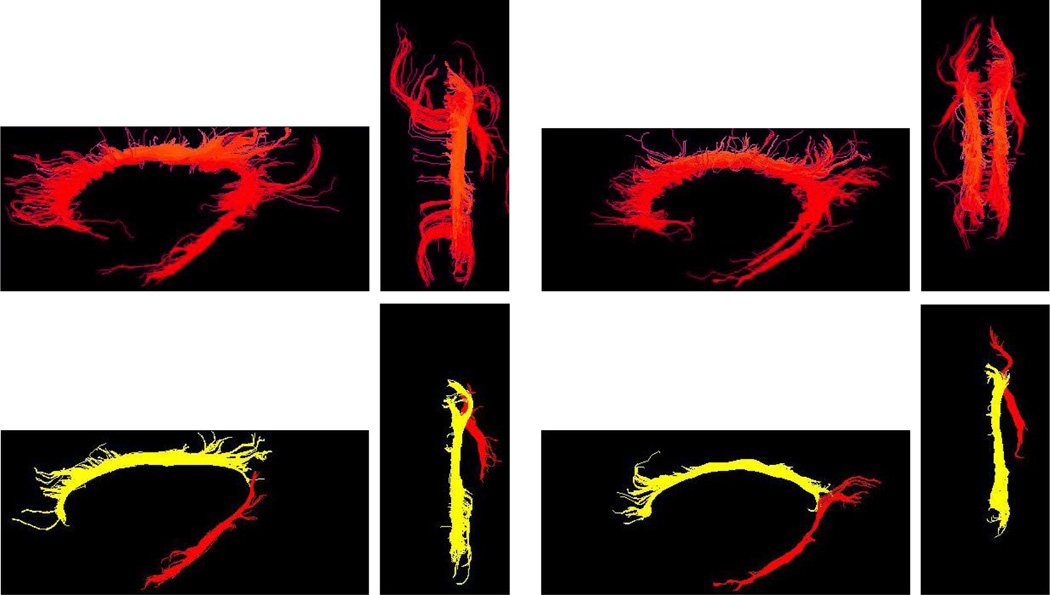
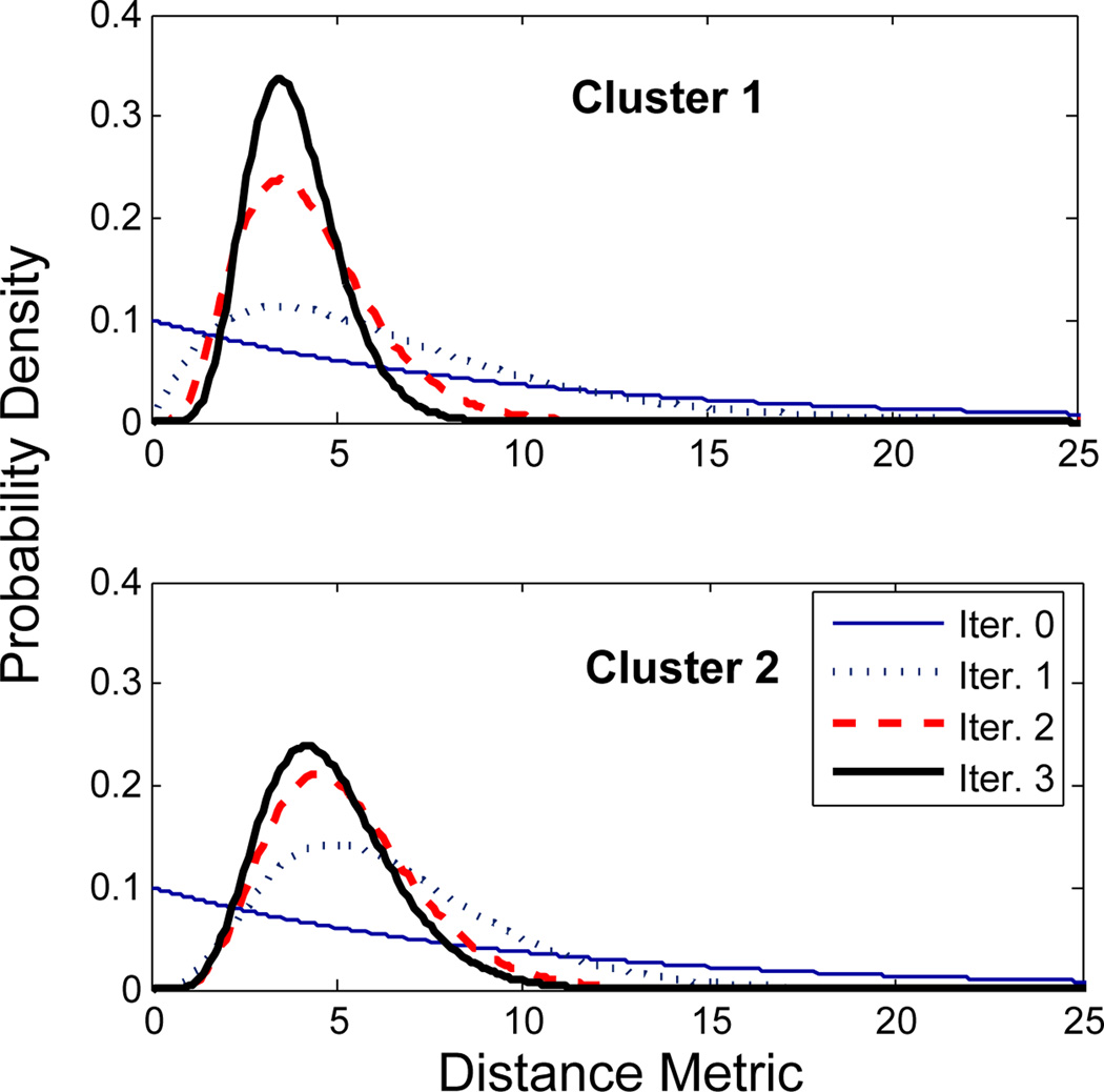
Fig. 2 shows the the results of clustering roughly 3000 trajectories from corpus callosum, middle cerebellar peduncle, corticobulbar, and corticospinal tracts into 25 bundles. As the initial centers, 25 trajectories from the data were selected manually, each representing an expected cluster. The membership probability of the trajectories to each cluster is obtained using the EM algorithm as described in Section 4. The trajectories in Fig. 2 are colored based on their maximum membership probabilities. One of the difficult bundles of fiber tracts to cluster is the cingulum. Even starting tractography from a user-defined ROI results in a set of disordered trajectories, mostly short in length because of low FA. Also, due to its adjacency to the corpus callosum, many callosal trajectories are included that adversely affect any further analysis of the bundle. As shown in Fig. 3 for two subjects, our method is well capable of clustering these trajectories into the desired bundles. Two arbitrary trajectories, one from the the superior and one from the posterior part of the cingulum were selected as the initial cluster centers. Knowledge of the point correspondence and hence rigorous calculation of the similarity measure is essential for clustering of such a disordered set of trajectories. Fig. 4 illustrates the evolution of the Gamma distribution for the clusters of the first case shown the Fig. 3. Convergence is achieved just after a few iterations of the EM algorithm. The Gamma distribution was initialized with α = 1, corresponding to a exponential distribution, to value those trajectories that have no distance to the initial cluster center. However, as the algorithm proceeds, the Gamma distribution evolves from a very broad distribution to a narrow distribution with small but non-zero mode.

Fig. 2.

About 3000 trajectories clustered to 25 user-initialized bundles. Clusters include different segments of the corpus callosum, tapetum, middle cerebellar peduncle, corticobulbar and corticospinal tracts, and different portions of thalamic radiation.

Fig. 3.

Clustering of cingulum trajectories (top) into 2 bundles (bottom) for two healthy subjects. Saggital and axial views are shown for each case. Two arbitrary trajectories from the superior and inferior parts of the left cingulum were selected as the initial centers.

Fig. 4.

Evolution of the Gamma distributions that describe the normalized distance metric for the two clusters shown on the left in Fig. 3. After just a few iterations, the distribution converges to a narrow distribution with small but non-zero mode.

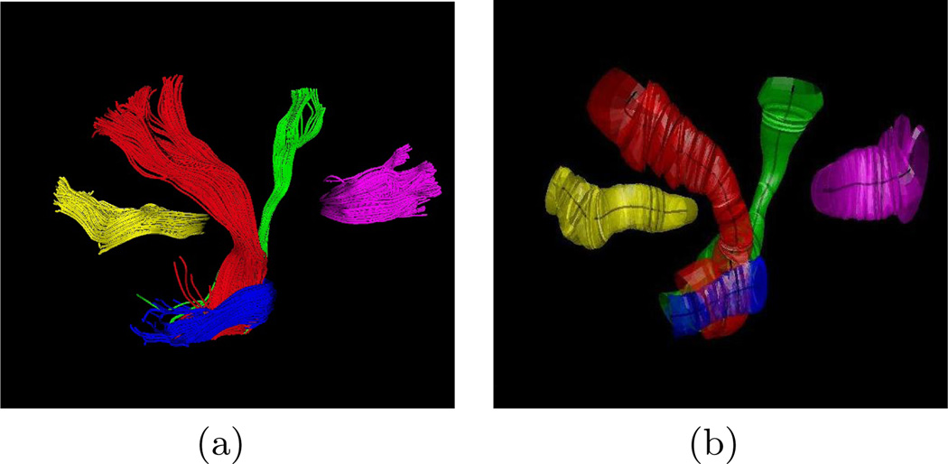
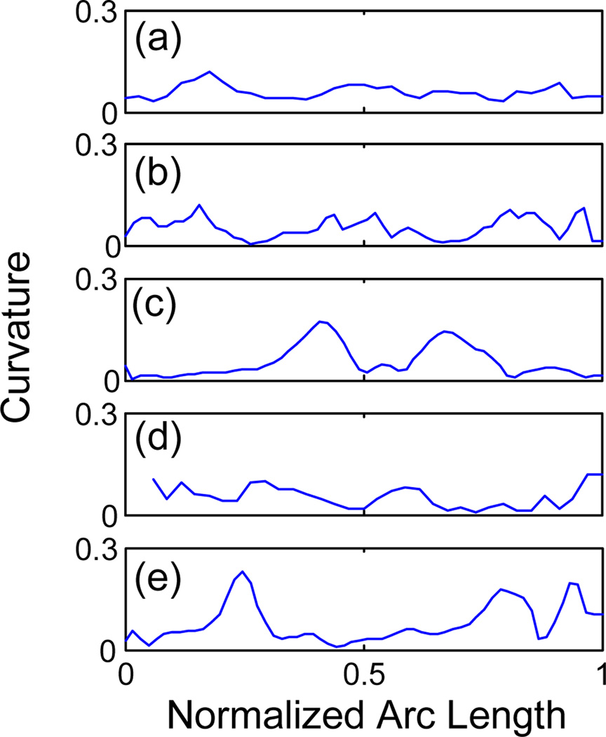
A spatial model of the fiber bundles represented by the mean trajectory and its spatial variation is also obtained. This is shown in Fig. 5 in which the abstract models of five fiber bundles are visualized by their spatial mean and isosurfaces corresponding to the mean plus three standard deviations (3σ) of the 3-D coordinates along the cluster center. Such an abstract spatial model for fiber bundles could be used for neurosurgery applications. It enables one to easily visualize the extent of the fiber tracts adjacent to the brain lesions to minimize the damage to the bundles when removing the lesion. Moreover, having the mean trajectory for each bundle of fiber tract allows us to study the shape of the bundle. As an example, the curvature versus the normalized arc length of the cluster centers are plotted in Fig. 6 for each cluster shown in Fig. 5.

Fig. 5.

(a) Trajectories of 5 different clusters used for quantitative analysis: splenium (yellow), corticospinal (red), corticobulbar (green), middle cerebellar peduncle (blue), and genu (magenta). (b) A model representation of the bundles as the mean trajectory and the isosurfaces corresponding to spatial variation of the clusters.

Fig. 6.

Curvature of the cluster center along its normalized arc length for fiber bundles shown in Fig. 5: (a) splenium, (b) genu, (c) middle cerebellar peduncle, (d) corticospinal, and (e) corticobulbar fiber tracts.

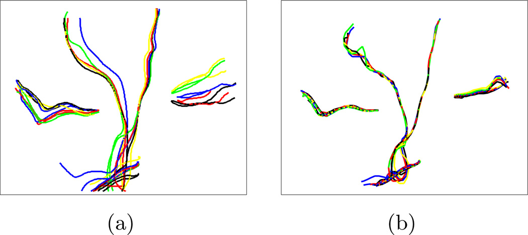
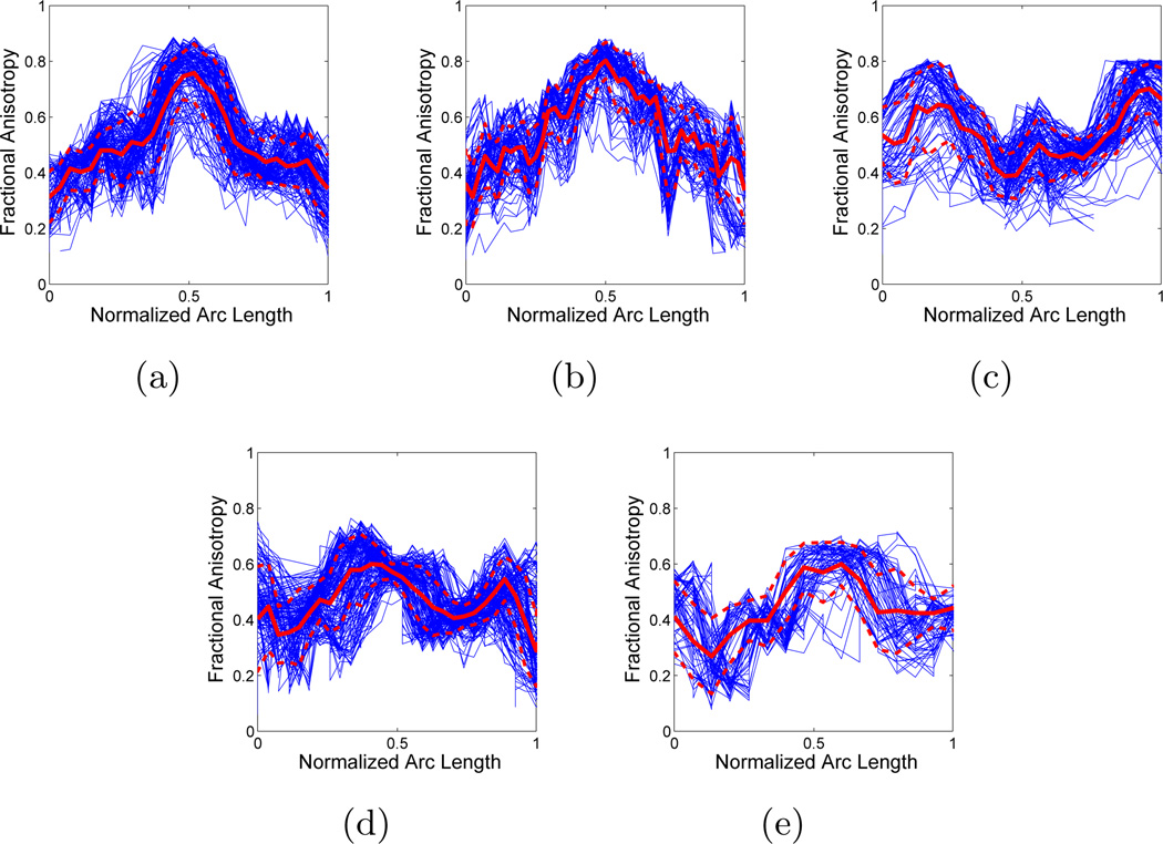
To investigate the sensitivity of the clustering to the initial centers, we randomly selected different sets of trajectories from each cluster shown in Fig. 5. At each run with one of the sets as the initial centers, the final centers obtained by the clustering algorithm are almost identical as shown in Fig. 7. This demonstrates the robustness of the algorithm with respect to the variations in the initial centers within each cluster. To demonstrate the suitability of our framework for tract-oriented quantitative analysis, we compute the mean and variation of the anisotropy parameters along the trajectories for clusters shown in Fig. 5. If any of anisotropy measures, such as fractional anisotropy (FA) and each of the three eigenvalues, or any of the local shape descriptors, such as curvature and torsion, are available along the trajectories, calculation of the mean and standard deviation of that parameter is quite straightforward. In fact, with the point correspondence obtained using the distance map described in Section 2, no further alignment of the quantitative parameters is necessary. Thus, similar to the computation of spatial mean and covariance of the clusters, performed in the M-stage of the EM algorithm, the mean and standard deviation of the parameters are obtained considering the membership probabilities of trajectories. Fig. 8 shows the mean and standard deviation of FA values along the normalized arc length of the cluster centers for each of the bundle in Fig. 5. To highlight the accuracy of our approach in aligning the fiber trajectories, the FA values along the aligned versions of all trajectories are also plotted (blue curves). These plots reveal the pattern of the FA values in the examined bundles.

Fig. 7.

Robustness of the EM algorithm with respect to the initial cluster centers. The algorithm was run 5 times with different initial centers (a) to cluster the trajectories in Fig. 5. Final cluster centers collected in (b) show little dependence on initial centers.

Fig. 8.

Fractional anisotropy vs. normalized arc length for fiber bundles in Fig. 5: (a) splenium, (b) genu, (c) middle cerebellar peduncle, (d) corticospinal, and (e) corticobulbar fiber tracts.

Being able to perform such an analysis is valuable since it enables us to study the local changes of quantitative parameters along the fibers. This is especially interesting for study of temporal changes of fiber tracts during brain development and also opens new possibilities to compare normal and pathological subjects. The unavailability of efficient tools for tract-oriented quantitative analysis has limited most clinical studies to date to evaluation of scalar averages of parameters over an ROI. Local variations that provide significant information about brain development [15] and pathologies [16] are thus lost in the course of study.

6 Conclusion

We demonstrated joint clustering and point-by-point mapping of white matter fiber trajectories using an EM algorithm in a Gamma mixture model context. The Gamma distribution enabled us to effectively model the normalized distance of the trajectories from each cluster center. Point correspondence of trajectories was obtained by constructing a distance map from each cluster centers at every EM iteration. This provides a time-efficient alternative to pairwise curve matching of all trajectories with respect to each cluster center. Probabilistic assignment of the trajectories to clusters was controlled with a minimum threshold on the membership posteriors, to offer flexibility in trading off between the robustness of the clusters and the number of outliers. Point correspondence calculated in our algorithm is an essential requirement of the tract-orientated quantitative analysis which is overlooked in previous works.

References

- 1.Gerig G, Gouttard S, Corouge I. Analysis of brain white matter via fiber tract modeling; Proc. IEEE Int. Conf. EMBS; 2004. [DOI] [PubMed] [Google Scholar]
- 2.Ruiz-Alzola J, Westin CF, Warfield SK, Nabavi A, Kikinis R. Nonrigid registration of 3D scalar, vector and tensor medical data; Int. Conf. on Medical Image Computing and Computer-Assisted Intervention; 2000. pp. 541–550. [Google Scholar]
- 3.Alexander DC, Pierpaoli C, Basser PJ, Gee JC. Spatial transformations of diffusion tensor magnetic resonance images. IEEE Trans. Med. Imag. 2001;20:1131–1139. doi: 10.1109/42.963816. [DOI] [PubMed] [Google Scholar]
- 4.Park HJ, Kubicki M, Shenton ME, Guimond A, McCarley RW, Maier S, Kikinis R, Jolesz FA, Westin CF. Spatial normalization of diffusion tensor MRI using multiple channels. NeuroImage. 2003;20:1995–2009. doi: 10.1016/j.neuroimage.2003.08.008. [DOI] [PMC free article] [PubMed] [Google Scholar]
- 5.Fillard P, Gerig G. Analysis tool for diffusion tensor MRI. Medical Image Computing and Computer-Assisted Intervention. 2003:967–968. doi: 10.1007/11566465_17. [DOI] [PubMed] [Google Scholar]
- 6.Shimony JS, Snyder AZ, Lori N, Conturo TE. Automated fuzzy clustering of neuronal pathways in diffusion tensor tracking. Proc. Int. Soc. Mag. Reson. Med. 2002:10. [Google Scholar]
- 7.Brun A, Knutsson H, Park HJ, Shenton ME, Westin CF. Clustering fiber tracts using normalized cuts; Seventh Int. Conf. on Medical Image Computing and Computer-Assisted Intervention; 2004. pp. 368–375. [DOI] [PMC free article] [PubMed] [Google Scholar]
- 8.O’Donnell L, Westin CF. White matter tract clustering and correspondence in populations; Eighth Int. Conf. on Medical Image Computing and Computer-Assisted Intervention; 2005. pp. 140–147. [PubMed] [Google Scholar]
- 9.Ding Z, Gore JC, Anderson AW. Classification and quantification of neuronal fiber pathways using diffusion tensor MRI. Mag. Reson. Med. 2003;49:716–721. doi: 10.1002/mrm.10415. [DOI] [PubMed] [Google Scholar]
- 10.Batchelor P, Calamante F, Tournier JD, Atkinson D, Hill DL, Connelly A. Quantification of the shape of fiber tracts. Magn. Reson. Med. 2006;55:894–903. doi: 10.1002/mrm.20858. [DOI] [PubMed] [Google Scholar]
- 11.Corouge I, Fletcher PT, Joshi S, Gouttard S, Gerig G. Fiber tract-oriented statistics for quantitative diffusion tensor MRI analysis. Med. Image Anal. 2006;10 doi: 10.1016/j.media.2006.07.003. [DOI] [PubMed] [Google Scholar]
- 12.Maddah M, Grimson WEL, Warfield SK. Statistical modeling and EM clustering of white matter fiber tracts; IEEE Int. Symp. Biomedical Imaging; 2006. [Google Scholar]
- 13.Hogg RV, Craig AT. Introduction to Mathematical Statistics. 4th edition. New York: Macmillan; 1978. [Google Scholar]
- 14.Basser P, Pajevic S, Pierpaoli C, Duda J, Aldroubi A. In vivo fiber tractography using DT-MRI data. Magn. Reson. Med. 2000;44:625–632. doi: 10.1002/1522-2594(200010)44:4<625::aid-mrm17>3.0.co;2-o. [DOI] [PubMed] [Google Scholar]
- 15.Berman JI, Mukherjee P, Partridge SC, Miller SP, Ferriero DM, Barkovich AJ, Vigneron DB, Henry RG. Quantitative diffusion tensor MRI fiber tractography of sensorimotor white matter development in premature infants. NeuroImage. 2005;27:862–871. doi: 10.1016/j.neuroimage.2005.05.018. [DOI] [PubMed] [Google Scholar]
- 16.Goldberg-Zimring D, Mewes AUJ, Maddah M, Warfield SK. Diffusion tensor magnetic resonance imaging in multiple sclerosis. J. Neuroimaging. 2005;15:68S–81S. doi: 10.1177/1051228405283363. [DOI] [PubMed] [Google Scholar]