The Relevance Voxel Machine (RVoxM): A Bayesian Method for Image-based Prediction

Abstract

This paper presents the Relevance Voxel Machine (RVoxM), a Bayesian multivariate pattern analysis (MVPA) algorithm that is specifically designed for making predictions based upon image data. In contrast to generic MVPA algorithms that have often been used for this purpose, the method is designed to utilize a small number of spatially clustered sets of voxels that are particularly suited for clinical interpretation. RVoxM automatically tunes all its free parameters during the training phase, and offers the additional advantage of producing probabilistic prediction outcomes. Experiments on age prediction from structural brain MRI indicate that RVoxM yields biologically meaningful models that provide excellent predictive accuracy.

1 Introduction

Medical imaging commonly entails relating image content to a clinical or experimental condition. Traditional univariate approaches, such as voxel-based morphometry [1] or cortical thickness analysis [2], can generate anatomical maps of the effects by analyzing each location individually. Multivariate pattern analysis (MVPA) methods, in contrast, offer dramatically increased specificity and sensitivity for predicting a clinical or experimental condition of interest by considering all voxels simultaneously [3–9]. However, studies in the field of image-based prediction have typically employed generic MVPA methods, such as Support or Relevance Vector Machines (SVMs/RVMs) [10, 11], which do not take into account the spatial organization inherent in imaging data.

As demonstrated in the area of semi-supervised learning, significant performance gains can be obtained by explicitly utilizing the underlying structure of the data at hand [12, 13]. One approach to achieve this in the context of images is to impose an a priori model on the covariation of voxel-level measurements – a strategy that has proven powerful for many computer vision problems [14]. Additional motivation for such models in the context of image-based prediction is interpretability: rather than a “black box” tool, we are also interested in understanding and visualizing the key areas that are driving predictions. Although it is possible to display the workings of generic linear MVPA methods as images [6], the results are often scattered and hard to interpret biologically [15].

In this paper, we present the Relevance Voxel Machine (RVoxM), a novel MVPA algorithm that is specifically designed for making and explaining image-based predictions. It uses a Bayesian modeling approach and builds largely on existing RVM machinery to obtain not only good prediction performance, but also sparse solutions. Unlike RVMs, however, where sparseness is realized by discarding many of the samples, i.e., subjects in the training dataset, our approach removes most of the voxels, retaining only those voxels that are relevant for prediction. Furthermore, our model encourages spatial clustering of these “relevance voxels” and computes predictions as linear combinations of their content, yielding results that are both biologically plausible and intuitive to interpret. Compared to related efforts that incorporate spatial context within the SVM framework [15], our method inherits all the usual advantages of RVMs over SVMs, including the benefits of probabilistic outcomes and the automatic tuning of all free parameters.

We test RVoxM on the problem of estimating the age of healthy subjects from structural brain MRI scans, and show that it achieves high accuracy using a pattern of “relevance voxels” that easily lends itself to biological interpretation.

2 Model

We use a generative model similar to the one of RVM [11]. Let t denote a real-valued target variable (e.g., age) that we aim to predict from image data, and x_i a voxel-level measurement (e.g., gray matter density) at the voxel indexed by i. We define a Gaussian conditional distribution for $t:p(t\mid \mathbf{x},\mathbf{w},\beta )=\mathcal{N}(t\mid y\left(\mathbf{x}\right),{\beta }^{-1})$, with variance β⁻¹ and a mean that is given by the linear model

$$y\left(\mathbf{x}\right)=\sum _{i=1}^M{x}_i{w}_i+w_0={\mathbf{w}}^{\text{T}}\mathbf{x},$$ (1)

where w = (w₀ … w_M)^T are adjustable “weights” encoding the strength of each voxel's contribution to the prediction, x = (1, x₁, … , x_M)^T denotes the vectorized image the prediction is based on, and M is the number of voxels. For notational convenience, we include an extra “voxel” to account for the bias, w₀.

For reasons that will soon become clear, we further assume a zero-mean Gaussian prior distribution over w:

$$p(\mathbf{w}\mid \mathbf{\alpha },\lambda )=\mathcal{N}(\mathbf{w}\mid \mathbf{0},{\mathbf{P}}^{-1}),$$

where P is a (M + 1) × (M + 1) precision (inverse covariance) matrix defined as

$$\mathbf{P}=\text{diag}({\alpha }_0,\cdots ,{\alpha }_M)+\lambda \mathbf{K}.$$

Here, α = (α₀, … , α_M) and λ are hyperparameters, and K is a fixed, positive-semidefinite matrix that encourages local spatial smoothness of w. In particular, we use K = Υ^TΥ, where Υ is a sparse matrix in which each row corresponds to a pair of neighboring voxels in the image. For neighboring voxels {i, j}, the corresponding row has zero entries everywhere expect for the i^thand j^th column, which have entries −1 and 1, respectively. Re-writing the prior as

$$p(\mathbf{w}\mid \alpha ,\lambda )\propto \text{exp}\left(-\frac{1}{2}\sum _{i=0}^M{\mathbf{\alpha }}_i{w}_i^2-\frac{\lambda }{2}{\Vert \mathbf{{\rm Y}}\mathbf{w}\Vert }^2\right)$$

shows that it encodes a preference for models that are both sparse and spatially clustered: we explicitly seek models that explain t through a small collection of image patches that easily lend themselves to neuroscientific interpretation. Indeed, the fact that there is an individual hyperparameter α_i associated with each voxel's weight w_i is responsible for achieving sparsity in those weights – as we shall see, estimating the α_i's automatically sets many of them to very large values, forcing the corresponding weights to zero and therefore “switching off” the contribution of many voxels. Importantly, we also explicitly take the spatial structure of image data into account by penalizing large entries in the vector Υw, which represent large differences between the weights of neighboring voxels. Thus, we encode a preference for spatial clusters of “switched-on” voxels, as these are both biologically more plausible and easier to interpret than speckles of isolated voxels scattered throughout the image area.

3 Hyperparameter Estimation

Given training data in the form of a set of N input-target pairs ${\{{\mathbf{x}}_n,t_n\}}_{n=1}^N$ where x_n represents the n^th training image and t_n the corresponding target variable, our first goal is to determine the values of the hyperparameters α, λ, and β. Using type-II maximum likelihood, we estimate the hyperparameters by maximizing the marginal likelihood function obtained by integrating out w:

$$\begin{array}{cc}\hfill p(t\mid \mathbf{X},\mathbf{\alpha },\lambda ,\beta )& ={\int }_{\mathbf{w}}\left(\prod _{n=1}^{N}p(t_n\mid {\mathbf{x}}_n,\mathbf{w},\beta )\right)p(\mathbf{w}\mid \mathbf{\alpha },\lambda )d\mathbf{w}\hfill \\ \hfill & ={\int }_{\mathbf{w}}{\left(\frac{\beta }{2\pi }\right)}^{N∕2}\text{exp}(-\frac{\beta }{2}{\Vert t-\mathbf{Xw}\Vert }^2)\frac{\mid P{\mid }^{1∕2}}{{\left(2\pi \right)}^{M∕2}}\text{exp}(-\frac{1}{2}{\mathbf{w}}^T\mathbf{P}\mathbf{w})d\mathbf{w}\hfill \\ \hfill & =\frac{\mid \mathbf{\Gamma }{\mid }^{-1∕2}}{{\left(2\pi \right)}^{N∕2}}\text{exp}(-\frac{1}{2}{\mathbf{t}}^T{\mathbf{\Gamma }}^{-1}\mathbf{t}),\hfill \end{array}$$ (2)

where t = (t₁, … , t_N)^T, X = [x₁, … , x_N]^T is the N × (M + 1) “design” and matrix, and we have the N × N matrix Γ given by

$$\mathbf{\Gamma }={\beta }^{-1}\mathbf{I}+{\mathbf{XP}}^{-1}{\mathbf{X}}^T.$$

We take a “coordinate-ascent” approach to search for the hyperparameters that maximize Eq. (2). Fixing λ, β, and {α_j} for all j ≠ i, differentiating the log of Eq. (2) w.r.t α_i, equating to zero and rearranging yields the following update:

$${\alpha }_i^{new}=\frac{{\Delta }_{ii}}{{\mu }_i^2}{\alpha }_i,$$ (3)

where

$$\mathbf{\mu }=\beta \mathbf{\Sigma }{\mathbf{X}}^T\mathbf{y},\Sigma ={(\beta {\mathbf{X}}^T\mathbf{X}+\mathbf{P})}^{-1},$$ (4)

and Δ is defined as Δ = P⁻¹ − Σ. Similarly, fixing α and β, differentiating w.r.t λ, and rearranging yields the following update equation for λ:

$${\lambda }^{\text{new}}=\frac{\text{trace}\left(\mathbf{\Delta }\mathbf{K}\right)}{{\mathbf{\mu }}^{\prime }\mathbf{K}\mathbf{\mu }}\lambda .$$ (5)

Finally, an update for β can be computed using the same approach:

$${\beta }^{new}=\frac{N}{{\Vert \mathbf{y}-\mathbf{X}\mathbf{\mu }\Vert }^2+\text{trace}\left(\mathbf{X}\mathbf{\Sigma }{\mathbf{X}}^T\right)}.$$ (6)

Optimization now proceeds by cycling through these equations. We monitor the value of the objective function of Eq. (2) and terminate the algorithm when the increase over the previous iteration is below a certain tolerance. Although currently we have no theoretical guarantees that the presented update equations indeed increase the objective function at each iteration, we have not encountered any situation where this was not the case during the course of our experiments.

4 The RVoxM Learning Algorithm

In practice, we find that most α_i's tend to grow to infinity during the optimization process, effectively clamping the corresponding weight w_i's to zero and removing those voxels from the model. We exploit this fact to obtain a greedy learning algorithm that is fast enough to be applied to large 3-D image volumes, using two computational tricks.

First, each time one of the α_i's exceeds a certain (very large) value, the corresponding voxel is pruned from the model and computations continue based on the remaining voxels only, in a manner similar to the RVM learning algorithm in [11]. Second, we use a multi-resolution approach commonly employed in image processing applications (e.g., [16]). We first construct a pyramid representation of the training images, where each level consists of lower-resolution images computed by subsampling the images from the previous resolution. The algorithm then starts by learning the hyperparameters for the lowest resolution images, propagates them down for the initialization of the next level, and so forth until the final resolution level is reached; voxels that were pruned at the previous level remain so at the current level as well.

Although this greedy algorithm prevents voxels from re-entering once they have been removed, our experiments suggest that it works quite well in practice.

5 Using RVoxM to Make Predictions

Once we have learned the hyperparameters α*, λ*, and β* from the training data, we can make predictions about the target variable t for a new input image x by evaluating the posterior

$$p(t\mid \mathbf{x},\mathbf{X},\mathbf{t},{\mathbf{\alpha }}^{\ast },{\lambda }^{\ast },{\beta }^{\ast })={\int }_{w}p(t\mid \mathbf{x},\mathbf{w},{\beta }^{\ast })p(\mathbf{w}\mid \mathbf{X},\mathbf{t},{\mathbf{\alpha }}^{\ast },{\lambda }^{\ast })d\mathbf{w}.$$

It can be shown that this distribution is a Gaussian with mean

$${\mathbf{\mu }}^T\mathbf{x}$$ (7)

and variance $\frac{1}{{\beta }^{\ast }}+{\mathbf{x}}^T\mathbf{\Sigma }\mathbf{x}$ where μ and Σ are given by Eq. (4) in which α, λ, and β have been set to their optimized values α*, λ*, and β*.

In the remainder, we will use the maximum a posteriori (MAP) value given by Eq. (7) to make predictions about t, which corresponds to the linear prediction model of Eq. (1) in which the voxels' weights w have been set to μ. It is worth emphasizing that in many voxels μ_i = 0 (because their α_i was set to infinity) – we call the remaining voxels the “relevance voxels” as these are the only ones effectively used to predict the target variable t.

6 Experimental Results

We applied RVoxM to the problem of estimating a person`s age from a brain MRI scan. This problem has attracted recent attention [17–19] since it provides a novel perspective for studying healthy development and aging patterns, while characterizing pathologic deviations in disease.

We used a collection of T1-weighted scans from 336 cognitively normal subjects (age range 18–93 years), available through the OASIS dataset⁴. We processed all the MRI scans with SPM8⁵, using default settings, to obtain spatially aligned gray matter maps for each subject. The gray matter density values (tissue probabilities modulated by the Jacobian of the non-linear warp) were used as the voxel-level measurements x_i in the remainder of the experiment. To assess generalization accuracy, we split the data into two arbitrary⁶ halves that are age and sex matched (43.7 ± 23.8 years, 62.5% female). We employed each group to train the RVoxM, which was then applied to the complementary group for testing. All reported results are averages across the two training/testing sessions.

In addition to RVoxM, we used two other methods as benchmarks. The first method, referred to as “RVM”, is another approach for estimating age from structural MRI [19]. It uses a principal component analysis (PCA) to achieve a dimensionality-reduced representation of the image data, and subsequently applies a linear RVM algorithm in the resulting feature space. We used the optimal implementation settings that were described in [19] and a public implementation of RVM⁷. The second benchmark (“RVoxM-NoReg”) was an implementation of RVoxM with no spatial regularization, i.e., with the hyperparameter λ intentionally clamped to zero. A comparison with the latter benchmark gives us an insight into the effect of spatial regularization on the results.

Fig. 1 (top left) illustrates the root mean square error achieved with the three algorithms. On average, RVoxM yields the best accuracy with a root mean square error of less than 9.5 years; Fig. 1 (bottom left) plots the age predicted by RVoxM for each subject versus the subject`s real age. Fig. 1 (top right) plots the average difference between the individual-level prediction errors (square of predicted age minus true age) obtained by RVoxM and the other two methods. On average, RVoxM achieves a statistically significantly smaller prediction error at the individual-level. RVoxM also attains the highest correlation (r-value) between the subjects' real age and predicted age among all three methods: 0.92 for RVoxM vs. 0.90 and 0.91 for RVM and RVoxM-NoReg, respectively.⁸

Fig. 1.

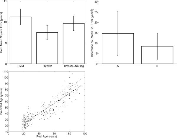
Top Left: Average root mean square error for the three MVPA methods. Top Right: Average difference between subject-level prediction errors, measured as square of real age minus predicted age. (A) Error of RVM minus error of RVoxM. (B) Error of RVoxMNoReg minus error of RVoxM. Error bars show standard error of the mean. Bottom Left: Scatter plot of age estimated with RVoxM versus real age.

Fig. 2 shows μ, RVoxM`s estimated voxel weights, for each of the two training sessions. Recalling that the prediction on new data is simply the linear product between μ and the test image (Eq. (7)), the value of μ at a specific voxel reflects the contribution of that voxel to the prediction. It can be appreciated that most voxels have a zero contribution (i.e., the model is sparse), and that the “relevance voxels” (with a non-zero contribution) occur in clusters, providing clear clues as to what parts of the gray matter are driving the age prediction process. Furthermore, the relevance voxels exhibit an overall very similar pattern across the two training sessions, providing evidence that these patterns are likely to be associated with the underlying biology and can be interpreted. We leave the interpretation of these relevance voxel patterns to future work.

Fig. 2.

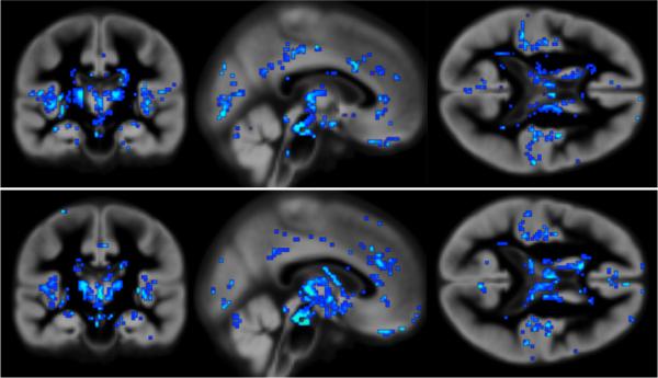
Relevance voxels (in blue) for predicting age, overlaid on the average gray matter density image across all subjects. Brighter blue indicates a higher absolute value, and thus a higher relevance for prediction. Top row: Model from training on the first half of the data. Bottom row: Model from training on the second half of the data.

7 Conclusion

In this paper, we proposed a novel Bayesian framework for image-based prediction. The proposed method yields a model where the predicted outcome is a linear combination of a small number of spatially clustered sets of voxels. We developed a computationally efficient optimization algorithm, RVoxM, to learn the properties of this model from a training data set. While RVoxM is not guaranteed to find the global optimum, our empirical results suggest that it finds a good solution in practice. Experiments on age prediction from structural brain MRI indicate that RVoxM derives excellent predictive accuracy from a small pattern of voxels that easily lends itself to neuroscientific interpretation.

Although we have used a regression model in this paper, it is straightforward to extend the technique to probabilistic classification by introducing a logistic sigmoid function [11]. In future work, we thus intend to apply RVoxM to also predict dichotomous outcomes (e.g., diagnosis), in addition to continuous ones.

References

- 1.Ashburner J, Friston KJ. Voxel-based morphometry-the methods. Neuroimage. 2000;11(6):805–821. doi: 10.1006/nimg.2000.0582. [DOI] [PubMed] [Google Scholar]
- 2.Fischl B, Dale AM. Measuring the thickness of the human cerebral cortex from magnetic resonance images. PNAS. 2000;97(20):11050. doi: 10.1073/pnas.200033797. [DOI] [PMC free article] [PubMed] [Google Scholar]
- 3.Cox DD, Savoy RL. Functional magnetic resonance imaging (fMRI) “brain reading”: detecting and classifying distributed patterns of fMRI activity in human visual cortex. Neuroimage. 2003;19(2):261–270. doi: 10.1016/s1053-8119(03)00049-1. [DOI] [PubMed] [Google Scholar]
- 4.Davatzikos C, et al. Detection of prodromal Alzheimer`s disease via pattern classification of MRI. Neurobiology of aging. 2008;29(4):514. doi: 10.1016/j.neurobiolaging.2006.11.010. [DOI] [PMC free article] [PubMed] [Google Scholar]
- 5.Fan Y, Batmanghelich N, Clark CM, Davatzikos C. Spatial patterns of brain atrophy in MCI patients, identified via high-dimensional pattern classification, predict subsequent cognitive decline. Neuroimage. 2008;39(4):1731–1743. doi: 10.1016/j.neuroimage.2007.10.031. [DOI] [PMC free article] [PubMed] [Google Scholar]
- 6.Kloppel S, et al. Automatic classification of MR scans in Alzheimer`s disease. Brain. 2008;131(3):681. doi: 10.1093/brain/awm319. [DOI] [PMC free article] [PubMed] [Google Scholar]
- 7.Magnin B, et al. Support vector machine-based classification of Alzheimers disease from whole-brain anatomical MRI. Neuroradiology. 2009;51(2):73–83. doi: 10.1007/s00234-008-0463-x. [DOI] [PubMed] [Google Scholar]
- 8.Pereira F, Mitchell T, Botvinick M. Machine learning classifiers and fMRI: a tutorial overview. NeuroImage. 2009;45(1):S199–S209. doi: 10.1016/j.neuroimage.2008.11.007. [DOI] [PMC free article] [PubMed] [Google Scholar]
- 9.Pohl K, Sabuncu M. Information Processing in Medical Imaging. Springer; 2009. A unified framework for mr based disease classification; pp. 300–313. [DOI] [PMC free article] [PubMed] [Google Scholar]
- 10.Cortes C, Vapnik V. Support-vector networks. Machine learning. 1995;20(3):273–297. [Google Scholar]
- 11.Tipping ME. Sparse bayesian learning and the relevance vector machine. Journal of Machine Learning Research. 2001;1:211–244. [Google Scholar]
- 12.Batmanghelich N, et al. IPMI. Springer; 2009. A general and unifying framework for feature construction, in image-based pattern classification; pp. 423–434. [DOI] [PubMed] [Google Scholar]
- 13.Belkin M, Niyogi P, Sindhwani V. Manifold regularization: A geometric framework for learning from labeled and unlabeled examples. The Journal of Machine Learning Research. 2006;7:2399–2434. [Google Scholar]
- 14.Li SZ. Markov random field modeling in image analysis. Springer-Verlag New York Inc; 2009. [Google Scholar]
- 15.Cuingnet R, et al. Spatial prior in SVM-based classification of brain images. Proceedings of SPIE. 2010;7624:76241L. [Google Scholar]
- 16.Thevenaz P, et al. A pyramid approach to subpixel registration based on intensity. Image Processing, IEEE Transactions on. 2002;7(1):27–41. doi: 10.1109/83.650848. [DOI] [PubMed] [Google Scholar]
- 17.Ashburner J. A fast diffeomorphic image registration algorithm. Neuroimage. 2007;38(1):95–113. doi: 10.1016/j.neuroimage.2007.07.007. [DOI] [PubMed] [Google Scholar]
- 18.Dosenbach NUF, et al. Prediction of Individual Brain Maturity Using fMRI. Science. 2010;329(5997):1358. doi: 10.1126/science.1194144. [DOI] [PMC free article] [PubMed] [Google Scholar]
- 19.Franke K, Ziegler G, Kloppel S, Gaser C. Estimating the age of healthy subjects from T1-weighted MRI scans using kernel methods: Exploring the influence of various parameters. NeuroImage. 2010;50(3):883–892. doi: 10.1016/j.neuroimage.2010.01.005. [DOI] [PubMed] [Google Scholar]