Noninvasive Assessment of Wall-Shear Rate and Vascular Elasticity using Combined ARFI/SWEI/Spectral Doppler Imaging System

Abstract

The progression of atherosclerotic disease is a complex process believed to be a function of the localized mechanical properties and hemodynamic loading associated with the arterial wall. It is hypothesized that measurements of cardiovascular stiffness and wall-shear rate (WSR) may provide important information regarding vascular remodeling, endothelial function and the growth of soft lipid-filled plaques that could help a clinician better predict the occurrence of clinical events such as stroke.

Two novel ARFI based imaging techniques, combined on-axis/off-axis ARFI /Spectral Doppler Imaging (SAD-SWEI) and Gated 2D ARFI/Spectral Doppler Imaging (SAD-Gated), were developed to form co-registered depictions of B-mode echogenicity, ARFI displacements, ARF-excited transverse wave velocity estimates and estimates of wall-shear rate throughout the cardiac cycle. Implemented on a commercial ultrasound scanner, the developed techniques were evaluated in tissue-mimicking and steady-state flow phantoms and compared with conventional techniques, other published study results and theoretical values. Initial in vivo feasibility of the method is demonstrated with results obtained from scanning the carotid arteries of five healthy volunteers. Cyclic variations over the cardiac cycle were observed in on-axis displacements, off-axis transverse-wave velocities and wall-shear rates.

I. INTRODUCTION

Despite significant investment into its treatment, cardiovascular disease (CVD) continues to remain a major health problem in the United States, causing approximately 800,000 deaths every year. A significant subset of CVD deaths is due to atherosclerosis and its complications. The most recent update from the American Heart Association estimates that approximately 130,000 Americans died from ischemic myocardial infarction in 2007 while an additional 140,000 died from ischemic stroke.¹ While the exact progression is not entirely understood, it is generally accepted that atherosclerosis is accompanied by localized changes in both the mechanical and hemodynamic properties of the arterial system.² Imaging technologies that are able to identify these changes prior to the onset of either significant vascular remodeling or clinical events may be beneficial in the medical management of cardiovascular disease.

Several ultrasound-based approaches have been proposed for imaging the material and mechanical changes that accompany atherosclerosis. Typically these methods measure the response of vascular tissue to either a physiological or a nonphysiological deformation. Examples of physiological-based methods include intravascular ultrasound (IVUS)³ and non-invasive vascular elastography (NIVE).⁴ In both approaches, the magnitude of tissue strain in response to the natural pulsation of the artery is used to classify plaque. For example, an area of high-strain may suggest a potentially vulnerable plaque.^3-12 Estimates of elastic modulus can be also computed from these strain measurements using a model based approach.^{11, 12} Alternatively, a nonphysiological source, such as acoustic radiation force (ARF), can be used to deform the tissue. ARF-based methods include shear-wave elasticity imaging (SWEI),^{13, 14} vibro-acoustography,¹⁵ shear-wave dispersion ultrasound vibrometry¹⁶ and acoustic radiation force impulse (ARFI) imaging.¹⁷

ARFI imaging is an ARF-based technique where the pulse length and/or intensity of conventional, ultrasonic pulses are increased in order to generate ARF significant enough to displace tissue to a measurable distance.¹⁷ Correlation or phase-shift estimation techniques are then used to estimate the resulting tissue deformation within the initial region of excitation (ROE).^{18, 19} Displacements induced using ARFI techniques are typically very small (< 20 μm), and recover relatively quickly following an ARF excitation (i.e., in several milli seconds). Most studies investigating the utility of ARFI imaging for quantifying the tissue properties use the displacement information as a qualitative indicator of stiffness. For example, greater displacements are assumed to reflect more compliant regions of tissue.^{17, 20} Despite the qualitative nature of the method, ARFI imaging has been demonstrated in both ex vivo human and porcine arterial tissue^21-23 and in vivo in both the carotid and lower limb vasculature^24-26 and has been shown to locally differentiate plaque material composition.^22-24 Current vascular ARFI imaging methods utilize ECG-gated and nonECG-gated techniques, to form co-registered, 2D ARFI displacement and B-mode images of arterial tissue.

A more quantitative assessment of tissue stiffness can be obtained by utilizing SWEI techniques. ¹³Like ARFI imaging, these approaches rely on ARF to generate deformation within tissue. Unlike ARFI imaging, SWEI techniques deform tissue outside the ROE through the generation and propagation of shear or elastic waves, whose velocity can be tracked using ultrasound and then related to a material property through a model.¹³ These techniques have been adapted for vascular imaging in ex vivo porcine arteries,^{23, 27-29} and more recently, in vivo in the carotid artery in humans.³⁰ ARF-induced velocities of mechanical waves in arteries are typically in the range of 3 m/s to 8 m/s,^{23, 27-29} are dispersive^{27, 30} and have been shown to vary with the nonlinear change in arterial elasticity that accompanies increased transmural pressure load.^{23, 27, 29-30} Estimates of arterial moduli derived from these velocities are typically on the order of hundreds of kPa^27,30 and for the human carotid have been reported to range from 80 kPa in diastole to 130 kPa in systole for shear modulus.³⁰

While most ARF-based elastography efforts have focused on quantifying the mechanical remodeling that accompanies atherosclerosis, it has also been recognized that hemodynamic factors can have a strong impact on the progression of cardiovascular disease.^31-35 One such factor is wall shear stress, and in particular, its effect on both plaque growth and rupture. Abnormally low values of wall shear stress (WSS) have been hypothesized to encourage atherogenesis by increasing the exposure time of the intima to atherogenic agents while also hindering the protective function of the endothelium.^31,32 In clinically-significant plaque, low WSS may lead to increased plaque growth while plaque exposed to high WSS may be more prone to rupture due to a gradual weakening of the plaque cap via hemodynamic ally-driven remodeling.^33-35

Both estimates of viscosity and wall shear rate (WSR) are needed to quantify WSS. Because viscosity can be challenging to measure noninvasively, many ultrasonic techniques to date have instead focused on measuring the WSR. One proposed approach is to measure the peak flow velocity at a single depth within the artery using conventional spectral Doppler (typically near the center of the lumen) and then estimate the WSR from the velocity data using a flow model.^{36, 37} Alternatively, WSR can be estimated by measuring the flow velocity at several depths in the artery and then computing the spatial derivative of the measured velocity profile near the wall.^38-41 Typically, these approaches use multi-gated spectral Doppler to characterize the flow velocity profile within the artery.⁴²

Given the promise shown by SWEI and ARFI methods and the clinical relevance of both arterial elasticity and hemodynamics (WSR/WSS) with regard to atherosclerosis and its complications, it would be useful to acquire spatially-matched elasticity information and WSR information within the same acquisition. While both ARFI/SWEI and spectral Doppler information could be obtained from separate scans, the benefit of using a combined approach is that the spatial registration between the collected information can be more easily preserved while also eliminating the need for switching between modalities. In this study, we describe a combined ARFI, SWEI and multi-gated spectral Doppler imaging system that is capable of providing concurrent assessment of WSR using spectral Doppler, and elasticity using on-axis ARFI and off-axis SWEI imaging techniques. New sequencing methods for combining radiation-force elastography and WSR estimation techniques are presented and evaluated in steady-state flow and tissue-mimicking phantoms. Finally, the techniques are demonstrated in vivo in the carotid arteries of five healthy volunteers.

II. IMAGING METHODS

Current cardiovascular ARFI imaging and SWEI sequences

ARFI imaging has been previously described by Nightingale et al.¹⁷ Most ARFI imaging pulse sequences consist of three pulse-types; excitation, reference and tracking pulses. The excitation pulses used to generate nonneglible ARF inside tissue are typically unapodized, higher-intensity and longer-duration (compared to B-mode pulses). Reference and tracking pulses are conventional M-mode pulses used for displacement tracking before and after an ARF excitation. A typical ARFI imaging sequence will have one (or several) reference pulses, an excitation pulse and an ensemble of tracking pulses distributed over several milliseconds. ^{17, 43} An ARFI-displacement dataset is then formed by repeating this sequencing laterally over a given region of interest (typically 20-100 lateral locations over 1-3 cm), and then estimating the displacement as a function of elapsed time following excitation for each spatial position within the ARFI field of view (FOV).⁴⁴

For cardiovascular ARFI applications, parallel-receive, parallel-transmit and multi-time techniques are used to reduce acquisition time. Parallel-receive techniques utilize parallel-receive beamforming to track multiple locations per ARF-excitation.⁴⁵ Parallel-transmit methods utilize multiple subapertures for the excitation pulses to simultaneously generate ARF at multiple lateral locations.⁴³ Multi-time techniques alternate tracking beams at several, nonadjacent locations, reducing acquisition time with a corresponding reduction in pulse repetition frequency (PRF) for a given location.⁴⁶ These techniques can reduce single-frame ARFI imaging acquisitions to 35-50 ms, allowing for frame rates (25-20 Hz) suitable for real-time imaging.⁴⁶ More recently, color-flow pulses have been interleaved with multi-time, parallel-transmit ARFI pulses, allowing for the simultaneous acquisition of B-mode, ARFI and color-flow Doppler imaging frames at frame rates up to 20Hz.⁴⁷

In contrast to ARFI imaging, which uses information within the ROE, SWEI uses displacement information from outside the ROE to estimate ARF-induced wave velocities. A tissue modulus can then be estimated by fitting the velocity data to a mechanical wave model. For example, for linear, isotropic materials, the velocity of the excited shear wave can be described by

$$C_T=\sqrt{\frac{\mu }{\rho }}$$ (1)

Equation (1) suggests that by measuring the shear wave velocity (C_T), and assuming a tissue density (ρ), one can also obtain an estimate of a material’s shear modulus (μ).¹³ For modeling elastic wave propagation in arterial tissue, the above relation is largely inaccurate and thus guided-wave models are more commonly used to relate ARF-induced wave velocities to arterial material properties. ^27,30

SWEI pulse sequences are conceptually similar to ARFI pulse sequences in that each ensemble includes reference, excitation and tracking pulses. The difference lies in the positioning of the reference and tracking pulses relative to the excitation pulse. Because the primary interest is in characterizing wave propagation outside the ROE, reference and tracking pulses are transmitted in regions outside the ROE, rather than inside the ROE as with ARFI imaging. Displacement data outside the ROE can be acquired at multiple locations using either a massively parallel receive beamforming system that can obtain 64+ receive lines per transmit event^{14, 30} or with superposition, where a different region is acquired per excitation event, and multiple ARF excitations are needed to track wave propagation within a desired FOV.^{48, 49}

Proposed beam sequences

The sequences described in the subsections below are modified versions of existing ARFI or SWEI sequencing techniques that have been adapted to provide estimates of WSR, spectral Doppler velocity, vascular wall displacement and ARF-induced transverse wave velocity (TWV).

1. Combined on-axis/SWEI Spectral-AKFI Doppler (SAD-SWEI) imaging

In a single frame, the SAD-SWEI imaging sequence acquires a 2D B-mode sweep, M-mode ARFI and SWEI data information. Using a 4:1 parallel-receive technique, displacements are tracked simultaneously at four lateral locations for each of two excitation beams used in each frame. For the first excitation, the leftmost receive beam of the parallel cluster is aligned with the excitation beam and used for tracking displacements within the ROE (on-axis) to collect M-mode ARFI information. The received echo of the left-center receive beam is ignored because it is spatially located in the ROE. Off-axis SWEI information is collected by the two rightmost receive beams that are located outside the ROE (off-axis). After a second excitation, which is offset from the first excitation by one millimeter, four equally-spaced parallel receive beams track tissue displacements outside the ROE for SWEI information.

By combining the received information from all tracking beams, both M-mode ARFI (on-axis) and SWEI (off-axis) information are obtained over two excitations. On-axis information is collected by a single receive beam after the first excitation. Six off-axis receive beams (two from the first excitation and four from the second excitation) are combined to provide estimates of off-axis tissue displacement vs. time after excitation at different lateral locations equally distributed over an approximately 4 mm tracking FOV. Both types of elasticity information (within and outside the ROE) are collected at rates ranging from 5 to 10 fps for 1 s followed by the acquisition of spectral Doppler information using four clustered parallel-receive beams at a single lateral location for 1 s. The specific frame rate of the blood velocity estimate is dependent upon the number of samples used at each time during the cardiac cycle and the specific Doppler PRF. A diagram of this pulse sequence is provided in figure 1.

FIG. 1.

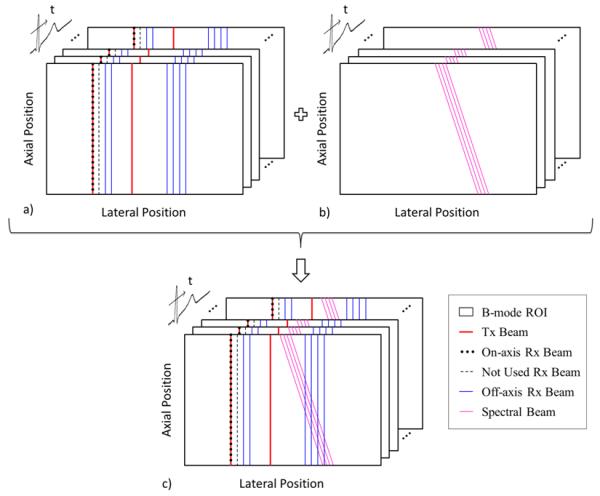
SAD-SWEI pulse-sequencing diagram with multiple frames of combined 2D B-mode, on-axis ARFI and off-axis SWEI beams (a), multiple frames of steered spectral Doppler pulses (b) and the combined multi-beat synthesized sequence. Spatial locations of beams are exaggerated for illustration.

2. Gated 2D Spectral-ARFI Doppler (SAD-Gated) imaging

An ECG-gated method was implemented to create a synthesized 3D (lateral position vs. axial position vs. time) image sequence of combined B-mode, ARFI and WSR depictions. Triggered on the QRS complex of the first heartbeat using the scanner’s internal ECG trigger, six interleaved B-mode and ARFI frames are acquired at 10 fps (approximately 50 ms per B-mode/ARFI frame, with a 50 ms delay between subsequent frames). Triggered on six subsequent heartbeats, spectral Doppler data is acquired for 600 ms simultaneously at three lateral locations spaced approximately 7 mm apart by implementing both parallel-transmit and parallel-receive techniques. Over the six heartbeats, this parallel-transmit scheme is walked across the array to obtain information at a total of 18 spectral Doppler locations over an approximately 20 mm FOV. Combining the received signals from each of the separate pulse gates creates a multi-beat synthesized sequence with spatially co-registeied triplex information. The final multi-beat synthesized image contains 128 lines for the B-mode image over a 38mm FOV, 44 lines for the ARFI image over a 20 mm FOV and 18 lines of spectral Doppler information over a 20 mm FOV. A diagram of this pulse sequence is provided in figure 2.

FIG. 2.

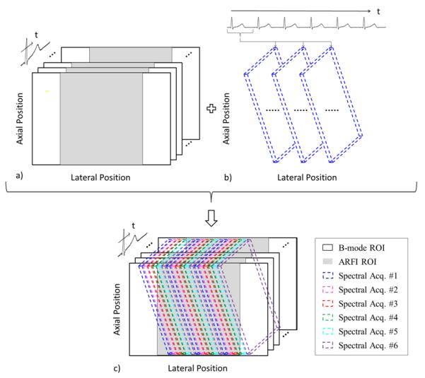
SAD-Gated pulse sequencing diagram with multiple frames of 2D B-mode and 2D ARFI collected during the first heartbeat (a), followed by the acquisition of 2D spectral Doppler at three lateral locations that are swept across the lateral FOV over six triggered heartbeats, with only the first spectral acquisition depicted (b), and the combined multi-beat synthesized sequence consisting of 2D B-mode, 2D ARFI, and 2D spectral Doppler (c). Spatial locations of beams are exaggerated for illustration.

Data collection

The combined ARFI/SWEI/Spectral Doppler pulse sequences were implemented on a Siemens SONOLLNE Antares^™ ultrasound system (Siemens Healthcare, Ultrasound Business Unit, Mountain View, CA) with the VF10-5 linear array transducer. The in-phase (I) and quadrature (Q) demodulated radiofrequency data were acquired using the Siemens Ultrasonic Research Interface^™ All data and image processing was performed offline.

ARFI imaging processing and display

On-axis ARF induced displacements were computed from the collected IQ data by estimating the relative phase shift between a reference (preexcitation) signal and successive (postexcitation) tracking signals for each lateral location using a phase-estimation algorithm.¹⁹ A quadratic-based motion filter was applied to remove artifacts from nonradiation force-induced motion, including physiological and transducer motion.⁴³

SWEI imaging processing and display

Estimates of shear wave velocity were obtained using the recently-developed Radon sum-estimation technique.⁴⁹ Briefly, motion filtered displacement data are extracted from a region of interestand arranged as a function of lateral position and time following shear-wave generation. The technique then considers all possible velocities bounded by the spatial-temporal domain of the data and integrates the data along apath described by each potential candidate velocity. The largest summation is then used as an estimate of the shear-wave velocity.⁴⁹ For phantom experiments, SAD-SWI velocity estimates are computed over an approximately 1 mm (axial) × 4 mm (lateral) kernel sampled with six equally-distributed tracking beams. For conventional SWEI, velocity estimates are computed over a similarly-sized kernel sampled with thirty tracking beams. For in vivo experiments, the kernel was reduced to five locations distributed over an approximately 3 mm lateral kernel to obtain a more localized velocity measurement.

Spectral velocity and wall shear-rate processing and display

Spectral velocity profiles were obtained by dividing the demodulated quadrature signal into multiple range gates (gate-size approximately 160 μm) and computing a frequency power spectrum for each gate using the Fast Fourier Transform (FFT).³⁸ A localized active contour algorithm was then used to automatically extract the peak frequency cross-sectional profile from the spectral data.⁵⁰ Velocities were then estimated from the extracted peak frequencies by

$$V=\frac{F_{\text{max}}c}{2f_0(\text{cos}\theta +\kappa \text{sin}\theta )}$$ (2)

where F_max is the peak detected frequency, c is the speed of sound,f₀ is the center frequency of the emitted pulse, θ is the Doppler angle, and k is an adjustment factor based on the transverse Doppler equation that corrects for intrinsic spectral broadening.^{41, 51} For a nonsteered linear array, κ is approximately twice the F/# of the Doppler system. For a steered linear array, κ can be approximated as twice the beamwidth (measured orthogonal to the beam axis) near the transducer face. For the 15° steered (75° Doppler angle), F/4 system utilized here, κ was approximated to be 8.3.⁵¹

The resulting velocity profile describes the peak velocity detected within each gate and is a function of depth through the cross-section of the vessel. WSR was estimated by performing a regression analysis on the velocity profile data, computing the radial gradient analytically from the regression coefficients and then evaluating the resulting polynomial over the cross-sectional depth of the artery. The peak cross-sectional shear rate estimates were assumed to represent the proximal and distal WSR.^{38, 41} For the ECG-gated SAD sequences, WSR estimates were overlaid on the proximal and distal arterial walls in the B-mode image for display.

III. EXPERIMENTAL PROCEDURES

Spectral Doppler imaging and WSR evaluation

To assess the spectral performance of the proposed SAD sequences, a steady-state flow rig was constructed using a peristaltic pump (Masterflex L/S^™ Easy-Load, 7518-10 drive head), and 6.4 mm diameter silicone tubing (Masterflex L/S^™17). A flow reservoir containing 1.5 L of blood-mimicking fluid (BMF) (CIRS, Norfolk, VA) was connected to the pump using silicone tubing. Flow pulsatility was dampened within the system by attaching the outlet tubing of the pump to the inlet connection of a polyethylene container with 200 mL of dead volume. A four-foot section of silicone tubing was attached to the outlet connection of the dead volume container, mounted inside a water tank and then returned to the flow reservoir. The solution was degassed and mixed for approximately two hours by a magnetic stirrer to reduce inhomogeneities within the BMF. Table 1 describes the acoustical and hemodynamic properties of the BMF compared to human blood.

Table 1.

Acoustic and Hemodynamic Properties of the CIRS Blood-Mimicking Fluid

Property	Human Blood58	CIRS BMF
Viscosity [mPa s]	3	4±0.5
Velocity [m/s]	1583	1570±30
Attenuation [dB/cm/MHz]	0.15	<0.1

A VF10-5 transducer was then mounted on a translation stage and positioned over the tubing with the flow axis parallel to the array surface. The spatial position of the transducer was then adjusted until a maximum velocity was observed in the spectrogram. The angular orientation was checked by measuring the velocity of the flow using 90° spectral Doppler and adjusting the transducer’s axis until a symmetric spectral profile about the baseline was also observed in the spectrogram.

For each trial, the flow pump rate was adjusted and the output flow rate measured using timed volume collection. One-second SAD-SWEI acquisitions were then acquired using the parameters described in table 2 (Experiment I). Estimates of peak-flow velocity and proximal/distal WSRs were obtained using the methods outlined in section II. Flow and WSR performance was determined by computing the mean and standard deviation of the estimated peak velocity and WSR data and comparing the results to the theoretical values extracted from the measured flow rates, using a parabolic flow model

$$V=\frac{Q}{A}$$ (3)

$$WSR=\frac{8V}{D}$$ (4)

where the mean velocity (V) and WSR are both functions of the volumetric flow rate (Q), cross-sectional flow area (A) and tube diameter (D). For steady-state, parabolic flow, the peak velocity is approximately twice the mean velocity.

Table 2.

Experimental parameters for SAD-SWEI and SAD-Gated imaging

Experiment	1	2	3	4
Excitation Frequency [MHz]	5.71	6.67	6.67	5.71
Excitation F/#	3.0	2.3	2.3	3.0
Axial Focus [mm]	18	18	18	18
ARFI pulse length [μs]	52	67	67	52
Tracking Frequency [MHz]	8.00	8.00	8.00	8.00
Doppler Frequency [MHz]	5.71	-	5.71	5.71
Doppler F/#	4	-	4	4
Doppler PRF [kHz]	4.78	-	6.21	5.53
Doppler pulse length [μs]	0.7	-	0.7	0.7
Doppler angle	75°	-	75°	75°
Peak MI.3	-	-	1.6	1.4
Peak Combined-Scan ISPTA.3 [mw/cm2]	-	-	343	236

SAD-SWEI imaging of tissue-mimicking phantoms

SAD-SWEI imaging performance was evaluated by comparing SAD-SWEI derived measurements of shear-wave velocity with those obtained using conventional SWEI imaging sequences.⁴⁸ For each experiment, the transducer was mounted in a translation stage and positioned over one of five elastic, tissue-mimicking phantoms (CIRS, Norfolk VA) of varying stiffness (10 -107 kPa). SWEI measurements were then obtained at 15 independent locations within each phantom by translating the transducer 5 mm in elevation between acquisitions and obtaining an estimate of TWV for the right-traveling wave using the parameters described in table 2 (Experiment II for conventional SWEI, Experiment III for SAD-SWEI) and the Radon-sum method for velocity estimation described previously.⁴⁹

In vivo SAD and SAD-SWEI imaging of the common carotid artery

Initial feasibility of in vivo SAD-SWEI and SAD-Gated imaging was evaluated in five human volunteers (5 male, mean age 43, range 32-57) under a research protocol approved by the Duke University Institutional Review Board (IRB). All subjects gave informed consent as outlined by the Duke IRB.

Subjects were scanned in the supine position; the right common carotid artery (CCA) was identified using conventional duplex imaging and then imaged with SAD-SWEI and SAD-Gated using the parameters described in table 2 (Experiment III for SAD-SWEI, Experiment IV for SAD-Gated). Subjects Nl, N3-N5 were scanned approximately 3-4 cm from the carotid bifurcation. Subject N2 was scanned approximately 1 cm from the carotid bifurcation. For each acquisition, the transducer was positioned parallel to the flow axis of the artery and oriented until both arterial walls appeared orthogonal in the B-mode image. Global ECG and the voltage of the ARF-excitation power supply were recorded simultaneously with the SAD-SWEI and SAD-Gated data to help facilitate comparison between SAD-derived displacement, TWV and WSR data with cardiovascular function. The mechanical index (MI) is 1.6 for the SAD-SWEI sequence and 1.4 for the SAD-Gated sequence, which are below the regulatory limit of 1.9. The combined scan, derated spatial peak temporal average intensity (ISPTA.3) can be calculated by

$$I{}_{SPTA}=\sum _{overx,zi=0}^{\text{max}N}PII{}_i(x,0,z)SRF$$ (5)

where PII is the pulse intensity integral of the ith beam (whether a spectral Doppler, B-mode, Tracking or ARFI-excitation pulse) measured at (x, 0, z) and derated assuming an attenuation coefficient of 0.3 dB/MHz/cm. SRF is the maximum possible scan-repetition frequency. The combined scan ISPTA.3 is then determined by summing the peak PII contributions for all pulse types (Doppler/B-mode/M-mode tracking/ARF excitation) at each sequence’s SRF.⁵² The combined scan ISPTA.3 was determined to be 343 mW/cm² for the SAD-SWEI sequence and 236 mW/cm² for the SAD-Gated sequence, which are both lower than the regulatory limit of 720 mW/cm² for diagnostic vascular ultrasound.

Estimates of ARF-induced, proximal wall displacement; ARF-induced, proximal wall velocimetry; peak flow velocity; and WSR were computed for each SAD-SWEI acquisition (four to five acquisitions per subject, 10 TWV and on-axis estimates and 105 WSR estimates per acquisition). For the cyclic variability analysis, systole was defined as the temporal window beginning with the peak systolic-flow velocity and ending with the dicrotic notch observed in the spectral Doppler velocity trace. Diastole was defined as all data points immediately preceding the QRS complex by 300 ms or less. Mean on-axis ARFI displacement and ARF-induced wave velocity were then determined for each subset (diastole or systole) and analyzed for statistical significance on a per acquisition and a per subject basis using one way analysis of variance (ANOVA). Mean population statistics were determined by grouping all diastolic and systolic displacement and velocity estimates from each subject and repeating the ANOVA analysis over the combined systolic and diastolic datasets. The time between sequential SAD-SWEI acquisitions was approximately 45-60 s.

Two-dimensional ARFI and B-mode/WSR images were then reconstructed from the SAD-gated data. Composite images of B-mode and localized WSR were created by overlaying the WSR information onto the B-mode scan.

IV. RESULTS

Spectral-Doppler imaging evaluation

Figure 3 shows typical cross-sectional spectral frequency and computed WSR plots from the steady-state flow experiments. Figure 3a shows the cross-sectional spectral frequency for a flow rate of 680 mL/min. Figure 3b shows the extracted peak frequency data points (marked yellow circles) while figure 3c shows the estimated WSR curve computed from the peak frequency data. In this example, the computed maximum and minimum WSR values extracted from the velocity profiles are 395.1 s⁻¹ and −362.4 s⁻¹.

FIG. 3.

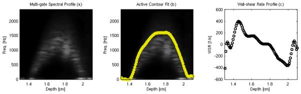
Sample cross-sectional velocity profile (a), fitted maximum frequency estim ate (b) and estimated WSR (c) from a steady-state flow rig using a flow rate of 680 mL/min.

Table 3 gives measured flow rates, computed theoretical mean and peak velocities and computed theoretical WSR values for the steady-state flow experiments. Figure 4a shows the peak velocities extracted from the SAD data (gray line) with error bars showing the mean and standard deviation of the peak velocity estimate plotted against the theoretical peak velocity (black line) computed using the measured flow rates. The mean relative error for the peak velocity measurement is 11% (range 1-23%), with a mean coefficient of variation of 10% (range 1-29%) between measurements. Overall, good agreement is observed between the theoretical and measured peak velocities.

Table 3.

Theoretical Flow Validation Data – 6.4mm Diameter Tube

Measured Flow Rate, [mL/min]	230	382	488	581	680	780	870
Computed Mean Velocity [cm/s]	11.9	19.8	25.3	30.1	35.2	40.4	44.9
Computed Peak Velocity [cm/s]	23.8	39.5	50.5	60.2	70.4	80.8	89.9
Computed WSR [1/s]	148.9	247.4	316.0	376.25	440.4	505.1	562.1

FIG. 4.

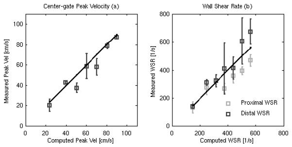
Estimated peak velocity (a) and WSR (b) measurements from the steady flow rate rig plotted against the theoretical flow velocities and WSRs calculated from the measured output flow rates. The dark line (a) shows the distal WSR measurement while the gray line (b) shows the proximal WSR measurement. Error bars give the mean and standard deviation across all measurements (n = 105).

Figure 4b shows the estimated proximal (light-gray line) and distal wall WSR (dark-gray line), with error bars showing the mean and standard deviation of the WSR estimates for each, plotted against the theoretical WSR (black line) derived from the measured flow rates. The mean relative error for the peak proximal WSR is 16% (range 3-29%), with a mean coefficient of variation of 15% (range 7-31 %). The mean relative error for the peak distal WSR measurement is 13% (range 2 -26%), with a coefficient of variation of 19%, range (6-45%). In general, good agreement is observed between theoretical and measured proximal and distal WSR measurements, except for at the highest flow rates, in which the proximal WSR results are smaller than the theoretical values and the distal WSR results are larger than the theoretical values.

SWEI measurements in phantoms

Figure 5 compares TWV measurements from the five CERS phantoms, with each point showing the mean and standard deviation for velocity estimates calculated using the Radon sum transformation for each sequence. Table 4 compares the mean and standard deviation of the velocity estimate from both sequences to the theoretical TWV calculated using Eq. (1) for each phantom. There is good agreement between the two sequences, with a correlation coefficient between velocities acquired using SAD-SWEI and SWEI greater than 0.97. However, the standard deviation of the TWV measurement is significantly higher for the SAD-SWEI sequences (mean 0.27, range 0.06-0.79) than the SWEI sequence (mean 0.06, range 0.02-0.15). In general, both sequences show good agreement with theoretical values, with an absolute mean error of 3.8 for the SWEI sequence and 3.2 for the SAD-SWEI sequence.

FIG. 5.

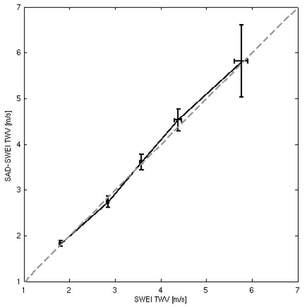
Estimated TWV measurements obtained using the SAD-SWEI sequence plotted against TWV measurements obtained using a conventional SWEI sequence, with the dashed gray line representing equality. Error bars give the mean and standard deviation from fifteen independent spatial locations within each phantom.

Table 4.

SWEI and SAD-SWEI Validation

Phantom	Stiffness [kPa]49	Calculated TWV [m/s]	SWEI TWV [m/s]	SAD-SWEI TWV [m/s]
A	9.8	1.81	1.79±0.02	1.82±0.06
B	23.9	2.82	2.84±0.02	2.74±0.13
C	44.2	3.84	3.57±0.04	3.61±0.17
D	67.3	4.73	4.38±0.08	4.53±0.24
E	107.1	5.97	5.76±0.15	5.82±0.79

In vivo SAD-SWEI and SAD-gated imaging of the common carotid artery

Figure 6a shows the spatial orientation of the ARF1 excitation beam (blue line), the on-axis measurement ROI (white box), the TWV measurement ROI (white dashed box) and the spectral Doppler beam (steered, green line) in relation to a B-m ode image of the common carotid and sample ARFI/S WEI/Spectral raw data for subject N2. Figure 6b shows the raw, center gate spectrogram as a function of time. Figures 6c-g show raw displacement vs. spatial position within the TWV measurement ROI as a function of time following excitation, with the gray lines showing the best Radon sum transform fit. Figure 6h shows the relative timing of the combined on-axis ARFI/TWV measurement (blue diamonds) and spectral Doppler measurements (green asterisks) with respect to the ECG trace.

FIG. 6.

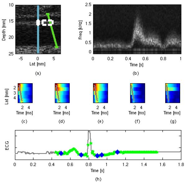
Spatial arrangement (a) of the ARFI excitation beam (blue line), on-axis measurement ROI (white box), off-axis TWV measurement ROI (dotted-white box) and spectral velocity ROI (green line) used for in vivo imaging. Sample extracted spectral Doppler frequency (b) plotted as a function of time. Sample raw displacement data used for the TWV estimate (c-g), with the greatest calculated Radon trajectories shown by the grey lines. Timing information (h) shows the temporal registration of the spectral Doppler estimates (green dots) and the ARFI/SWEI frames (blue dots) plotted against the global ECG trace (gray line).

Figure 7 shows WSR, ARFI, and TWV results for a typical acquisition taken from the same subject shown in figure 6 (N2). Figure 7a gives the estimated, center gate peak velocity (end diastolic velocity (EDV) = 0.16 m/s, peak systolic velocity (PSV) = 0.71 m/s) while figure 7b shows the estimated WSR for the proximal wall (black line, mean WSR = 254 s⁻¹, peak WSR = 511 s⁻¹) and distal wall (gray line, mean WSR = −285 s⁻¹, peak WSR = −792 s⁻¹). Both peak velocity and WSR are observed to increase sharply during vessel systole before tapering off through early andmid-diastole. Figure 7c shows the estimated ARF-induced wave velocity from the proximal wall. Figure 7d shows the estimated on-axis displacement in response to the radiation force, with lighter gray markers indicating greater elapsed time (0.45, 0.67, 0.90, 1.13, 1.35 ms, black – gray) after application of the radiation force). Changes in both ARF-generated TWV and on-axis displacement are observed between systole (i.e., the interval from peak flow velocity to the dicrotic notch) and diastole (i.e., the interval preceding the QRS complex in figure 7e). Figure 7e also shows the relative timing of the spectral data and the ARFI/TWV data with respect to the global ECG, with blue diamonds indicating an ARFI/TWV frame and green circles indicating a cross-sectional spectral estimate. Due to memory limitations, only one second of spectral data is collected in the SAD-SWEI sequence, leaving gaps in the velocity information from 0-0.4ms, and 1.6 - 1.8 ms as shown in the ECG trace.

FIG. 7.

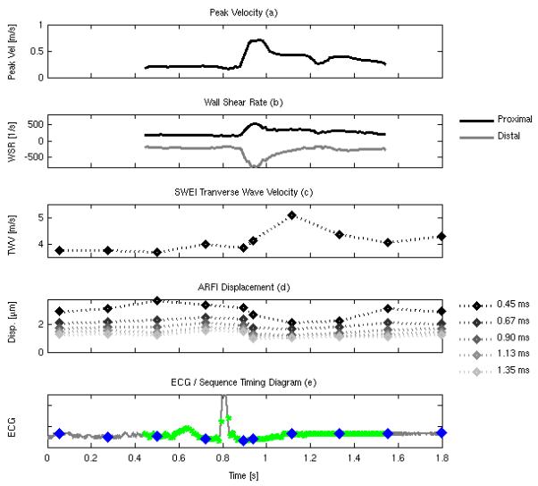
Peak flow velocity (a), estimated proximal (black line) and distal (gray line) WSR (b), estimatedTWV (c), on-axis displacement (d), with lighter symbols showing increased elapsed time following excitation (0.45, 0.67, 0.90, 1.13, 1.35 ms), and timing information (e) showing the temporal registration of the spectral Doppler estimates (green dots), the ARFI/SWEI frames (blue dots) plotted against the global ECG trace (gray line).

Table 5 summarizes the intrasubject variability for SAD-SWEI-derived flow velocity and WSR per subject and for the population as a whole. Average mean velocity for the five subjects was found to be 0.34±0.05 m/s (range 0.23-0.42 m/s) while average peak velocity was found to be 0.78 ± 0.12 m/s (range 0.63-1.07 m/s). Intrasubject coefficient of variation within the mean and peak velocity measurement was found to be 10 ± 4% for mean flow velocity measurement and 7 ± 2% for the peak flow velocity measurement. Average population mean WSR (average includes both walls) was found to be 296 ± 59 s⁻¹ (range 169-457 s⁻¹) while average peak WSR (average includes both walls) was found to be 722 ± 159 s⁻¹ (range 435 -1075 s⁻¹). Intrasubject coefficient of variation within the mean and peak WSR measurements was found to be 13 ± 3% for the estimates of mean WSR (range 9-17%), and 20 ± 5% for estimates of peak WSR (range 13-25%).

Table 5.

Summary of in vivo SAD hemodynamics data

Subject	Mean Vel [m/s]	Peak Vel [m/s]	Mean WSR [1/s]	Peak WSR [1/s]
N1	0.28±0.04	0.99±0.08	213.1±29.3	854.2±114.7
N2	0.35±0.05	0.69±0.05	280.7±23.8	608.8±139.6
N3	0.34±0.04	0.74±0.06	318.6±47.9	720.2±183.5
N4	0.34±0.04	0.71±0.06	328.7±56.2	687.4±159.6
N5	0.40±0.02	0.77±0.03	334.2±37.1	740.5±110.1
Population	0.34±0.05	0.78±0.12	296.2±59.4	722.1±159.9

Table 6 summarizes the intrasubject variability for diastolic and systolic TWV and on-axis displacement over five acquisitions per subject and for the population as a whole. Except for subject Nl (p = 0.48) and subject N2 (p = 0.05), a significant change in SWEI velocity was observed between diastolic and systolic velocity subsets (p<0.01 for N2-N4) and for the population as a whole (p<0.01). Mean TWV was found to be 4.1 ±0.6 m/s (range 1.6-5.1 m/s) during diastole and 4.7 ±1.1 m/s (range 2.2-10.9 m/s) during systole, with a mean change of +0.68 ± 0.3 m/s from diastole to systole. Statistically-significant changes in on-axis ARFI displacement (0.67 ms following force application) are observed between diastole and systole for all subjects and for the population as a whole (p <0.01). Mean diastolic on-axis displacement was found to be 1.7 ± 0.4 μm (range 0.95-2.9 μm) during diastole, and 1.1 ±0.4 μm (range 0.0-2.1 μm) during systole, with a mean change of −0.60 ± 0.2 μm from diastole to systole. In general, higher intrasubject measurement variation was found for TWV (18 vs. 16%) and on-axis ARFI displacement measurements (36 vs. 18%) obtained during systole.

Table 6.

Summary of in vivo SWEI and ARFI On Axis data

Subject	Diastolic SWEI [m/s]	Systolic SWEI [m/s]	p value	Diastolic on-axis [μm]	Systolic on-axis [μm]	p value
N1	2.9 ± 1.4	3.4 ± 1.0	0.48/NS	1.9 ± 0.5	1.1 ± 0.4	<0.01
N2	3.7 ± 0.3	4.5 ± 0.5	<0.01	2.0 ± 0.3	1.5 ± 0.4	<0.01
N3	3.9 ± 0.3	4.5 ± 0.4	<0.01	1.8 ± 0.3	1.0 ± 0.5	<0.01
N4	4.2 ± 0.3	4.7 ± 0.4	<0.01	1.6 ± 0.1	1.2 ± 0.3	<0.01
N5	4.6 ± 0.5	5.8 ± 1.9	0.05/NS	1.4 ± 0.3	1.0 ± 0.4	<0.01
Population	4.1 ± 0.6	4.7 ± 1.1	<0.01	1.7 ± 0.4	1.1 ± 0.4	<0.01

Figure 8a shows on-axis diastolic (black line) and systolic (gray line) displacements normalized to the peak diastolic displacement as a function of time following application of the radiation force. The error bars show the mean and standard deviation of the normalized diastolic and systolic displacement data over the entire study population. Figure 8b shows the normalized systolic data divided by the diastolic data over the same study population as a function of time following force application. Both plots suggests that a change in displacement between systole and diastole can be observed following ARF application, with the average systolic/diastolic ratio decreasing as the tissue recovers from the excitation. Note that standard deviations within the data appear to increase with increasing recovery time as the measured displacements gradually approach the noise floor.

FIG. 8.

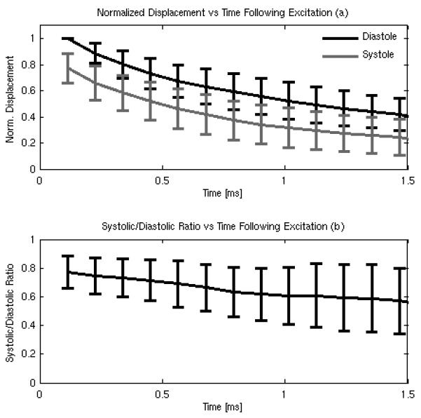
On-axis diastolic and systolic displacement (a) normalized to the peak diastolic displacement and the systolic/diastolic ratio computed from the normalized data (b) as a function of time. Error bars give the mean and standard deviation for the entire study population (n = 5 subjects).

Figure 9a shows the timing diagram for a S AD-Gated acquisition for subject N4, with the gray line showing the power supply voltage of the ultrasound scanner and the black line showing the ECG signal of the subject. Six frames of ARFI data are collected during the first heartbeat, followed by six frames of spectral velocity data over the next six heart beats. Figure 9b gives the final, reconstructed sequence plotted against the subject’s ECG, and shows the reconstructed timing between the 2D ARFI frames (blue diamonds) and the 2D Spectral/WSR frames (pink circles).

FIG. 9.

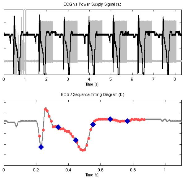
Top plot shows the temporal relationship between the global ECG (black line) and the SAD-Gated sequence power supply voltage (gray line). Six2D ARFI frames are acquired during the first heartbeat followed by six, 2D-synthesized spectral Doppler frames over six, sequential heartbeats. Bottom plot shows the timing relationship of the spectral Doppler estimates (light-red dots) and the ARFI estimates (blue diamonds) for the final, multi-beat synthesized sequence.

Figure 10 shows sample B-mode and WSR composite images (top row, a-d) and ARFI displacement images (middle row, e-h, and 0.78 ms following force application) for subject N4 reconstructed using the timing information shown in figure 9. The ECG trace in the bottom row gives the relative timing for the reconstructed frames, with pink circles indicating a B-mode/WSR frame and blue diamonds indicating an ARFI frame. The composite B-mode /WSR images show the temporal change in WSR loading on the proximal and distal arterial walls throughout the cardiac cycle, with peak WSR loading occurring prior to the T-wave. In the spatially co-registered ARFI image, both distal and proximal wall are well visualized, with a slight decrease in on-axis displacement (~0.5 urn) observed during the T-wave (figure 9g).Note that not every image is shown in the sequence due to the large volume of WSR images (54 frames) and ARFI images (6 frames) collected during the gated reconstruction.

FIG. 10.

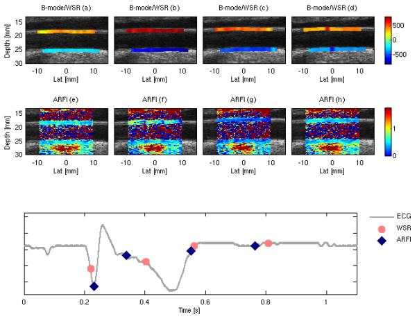
Multi-beat synthesized SAD-Gated depictions of WSR (values shown in s-1) overlaid on the B-mode image (top row) and 2D ARFI displacement (displacements shown in μm) images (middle row) of the common carotid artery for subject N4. The bottom plot shows the timing relationship between the ARFI frames (blue diamonds) and WSR frames (pink circles).

IV. DISCUSSION

This paper presents two new ultrasound based methods that allow for the noninvasive si-multaneous measurement of the hemodynamic and mechanical properties of the cardiovascular system. The first technique, SAD-SWEI imaging, allows for the estimation of on-axis ARFI displacement, off-axis ARF-induced velocimetry (SWEI/TWV), cross-sectional flow velocity and WSR loading on the proximal and distal wall. The second technique, SAD-Gated imaging, provides 2D, spatially co-registered depictions of WSR loading and ARF-induced displacements within the arterial wall throughout the cardiac cycle. To our knowledge, this represents the first demonstration for providing estimates of on-axis ARFI displacement, off-axis ARF-induced velocimetry and WSR data within a single acquisition using ultrasound based techniques.

Results from the flow phantom experiments indicate relatively good agreement between SAD-derived measurements of peak velocity and WSR with those predicted from the measured flow rates, with mean errors less than 17% for the WSR measurement and 11% for the peak velocity measurement. A noticeable bias toward higher WSR for the distal wall and lower WSR for the proximal wall is observed at higher flow rates, which may suggest that the inlet tube is not perfectly straight, skewing the flow profile and the WSR loading towards the distal wall.

Results from the SWEI phantom experiments show good agreement with both conventional SWEI and theoretical calculations derived assuming the phantoms are both linearly elastic and isotropic. However, SAD-SWEI derived phantom velocimetry measurements have significantly higher measurement variability, with a mean coefficient of variation approximately six times that of the SWEI sequence (6 vs. 1). This measurement variability becomes particularly noticeable at higher velocities (14 vs. 3 for TWV > 5 m/s). Given that SAD-SWEI attempts to reconstruct a ARE-induced wave velocity using only six tracking beams or less, it is not surprising to see a greater degree of measurement variability compared to conventional SWEI, which uses 24 beams or more.^48,49 While the Radon sum transformation was developed in part to improve velocity estimation in data corrupted by noise, noisy outliers from a single tracking location within a SAD-SWEI dataset will have a greater overall effect on dictating the optimal Radon sum and trajectory than a similar dataset constructed using a greater number of tracking locations, leading to a higher degree of variability for the velocity measurement. Implementing SAD-SWEI on a massively parallel-receive beamform ing system may help mitigate this variability, and improve performance to a similar order as currently realized SWEI techniques.^48,49

The population results in table 6 for peak and mean WSR are slightly lower compared to previous investigations into quantifying WSR using multi-gate techniques. Samijo et al investigated WSR variation as a function of gender and age over a population of 200 subjects (100 males, 100 females).³⁹ For the age distribution investigated in this study (30-59 years), Samijo et al reported peak WSR values ranging from 983 ± 188 s⁻¹ to 767 ± 114 s⁻¹ andmean WSR values ranging from 410 ± 83 s⁻¹ to 357 ± 81 s⁻¹ in male subjects. Tortoli et al reported peak and mean CCA WSR of 891 ± 167 s⁻¹ and 309 ± 72 s⁻¹ across a subject population (n = 16, gender not reported) ranging from 20-59 years old. Kornet et al noted higher WSR values in the proximal CCA (800-1010 s⁻¹) than near the bifurcation (677-754 s⁻¹) in 53 healthy subjects (age 18-67 years old). The population averages in this work across a similar age range for peak and mean WSR for all walls are 722 ± 160 s⁻¹ and 296 ± 59 s⁻¹. If the data from subject N2 (measured near the bifurcation as opposed to the proximal CCA) are excluded, the population averages are 749 ±154 s⁻¹ and 299 ± 65 s⁻¹, which are both lower than those reported by other groups for the CCA over a similar age range^{39-41, 53} and could be a reflection of the small study population, not measuring the flow velocities in the true areas of peak flow or an inherent bias in either the implemented multi-gate system or the active contour algorithm used for peak frequency extraction. The population numbers investigated herein are too small to facilitate comparing trends in WSR by age or location with previous results. The primary interest in this study was in vivo feasibility and more work usingareal-time version of the investigated system will be required to determine both the repeatability of the method over a large study population, the comparison of age, gender and location trends in WSR with previous work and whether the observed underestimation in WSR is inherent to the system or simply due to the lack of real-time feedback (for accurate gate placement) or limited subject numbers.

The variability in intrasubject WSR measurements using the SAD-SWEI system is higher than those reported by other groups⁴¹ and could be due to inadvertent operator/transducer drift in location or angle (or both) during the SAD-SWEI measurement. Currently, all processing of SAD-SWEI data is performed offline following the acquisition. Recent improvements in on-board GPU processing for motion tracking will likely support real-time processing of SAD-SWEI data, allowing for the sonographer to correct for drift by adjusting the probe in real-time until a maximum velocity is observed in the cross-sectional profile. Additionally, interleaving an additional Doppler beam orthogonal to the flow axis would allow for real-time correction of Doppler angle ambiguities during a SAD-SWEI acquisition, an approach that has been successfully implemented for flow velocity imaging and measurement of WSR.⁴¹ Given that current SAD-SWEI and SAD-Gated imaging acquisition times are limited by memory, such a system, however, would either require additional memory storage or adaptive spectral processing in order to reduce the number of ensembles required to form a single velocity profile to allow for the additional angle correction data.⁵⁴

Figure 7 demonstrates that flow velocity, WSR loading, on-axis ARFI displacement and ARF-induced velocimetry measurements can be acquired throughout the cardiac cycle using the same sequence. Both on-axis displacement and ARF-induced velocimetry measured using SAD-SWEI techniques show statistically-significant cyclic variability during the cardiac cycle, with higher wave velocities and lower displacements observed during vascular systole. This inverse relationship between decreased displacement and increased elastic wave velocity is not surprising, given that on-axis displacement dynamics within tissue are governed to a large degree by the elastic wave velocities supported by the insonified tissue.^20,55 Figures 7c, d demonstrate this relationship between on-axis displacement and ARF-induced velocimetry in arterial tissue, in which positive changes in ARF-induced wave speed during systole are observed to coincide with negative changes in the measured on-axis displacement. On average, we observe a +0.7 m/s change in ARF-induced wave velocity (mean normalized change of 18%), and −0.6 μm change in on-axis displacement (mean normalized change of 34%, 0.67 ms following excitation) within our initial study population, an observation that is consistent with a nonlinear increase in arterial elasticity from diastole to systole.

Discrepancies between the normalized magnitudes of the systolic-to-diastolic change observed by these metrics can also be explained in part by the same intrinsic relationship between on-axis displacement and ARF-induced wave mechanics. Figure 8a demonstrates that a noticeable decrease in displacement can be observed during systole for all time points (up to 1.5 ms) following excitation, which is consistent with an increased stiffness during systole. However, figure 8b also suggests that the relative ratio between systole and diastole for on-axis displacement changes with elapsed time following excitation, due to differential recovery times driven by differences in TWV during systole and diastole ^{20, 55} Similar trends have been reported in cardiac tissue by Bouchard et al, where it was observed that ratios of on-axis displacement become increasingly unstable with greater time following ARF excitation.⁵⁵ It is likely that due to the sensitivity of the time-point selected, the ARFI systolic/diastolic results presented here are more qualitative than quantitative, Despite this limitation, the smaller measurement kernel used for ARFI compared to SWEI (approximately an order of magnitude) makes the resolution offered by the on-axis information easily suitable for image formation.

It has been reported previously that guided waves propagating within arteries are dispersive, with the phase velocity of a given wave component dictated by its underlying frequency content.^27,30 The Radon-sum algorithm tracks the overall peak of the ARF-excited wave as it propagates across the ROI; velocities reported in this study reflect the group velocity of the wave, and would be bounded by phase velocities contained within the group.⁴⁹ Our primary interest was in evaluating the initial in vivo feasibility of obtaining ARFI/SWEI and WSR data using ultrasound and thus group velocity represents a simple metric for determining the initial in vivo feasibility for using a SAD-SWEI system. Previous investigations into ARF-induced TWV have reported ARF-induced group velocity values ranging from 4-6 m/s in an ex-vivo porcine aortas over the physiological range,²³ and ARF-induced phase velocities ranging from 3 -8 m/s for ex vivo and in vivo arteries, depending on the frequency chosen for analysis.^27,30 Our mean population velocity value, averaged over the cardiac cycle, is 4.4 m/s, which compares favorably to previous results. However, quantifying the entire dispersion behavior of the wave will likely be required to completely characterize the mechanical properties of the artery. Such an approach has been recently demonstrated using a broadband ARF excitation and a guided Lamb wave model.³⁰

Figure 10 demonstrates that 2D, spatially-registered images of WSR and ARFI displacement of the proximal CCA can be formed throughout the cardiac cycle using ECG-gated, SAD techniques. Although these images are from a different subject (N4 vs. N2), the 2D scan pairs illustrate similar temporal trends as the single line SAD-SWEI measurements shown in figure 7. In both examples, WSR is lowest before the QRS complex, rapidly increases during flow systole and then returns slowly to baseline during late systole and early-mid diastole. Interestingly, both figures 7 and 10 suggest that a phase difference exists between systolic flow (peak velocity and WSR) and peak systolic mechanical stiffness (SWEI and on-axis ARFI), with peak systolic flow velocity preceding the peak mechanical response. While such a result is consistent with alterations in pressure and flow waveforms due to reflected-wave augmentation,⁵⁶ it is unclear from these examples what the exact phase relationship is between the WSR and ARF-derived measurements (if any) given the sizeable difference in frame rate between the WSR measurement (>50 Hz) and the ARFI measurement (5-10Hz reconstructed). However, much higher frame-rates are possible, as a SAD-SWEI measurement can be formed in approximately 10 ms while a SAD-Gated ARFI image is formed in approximately 50 ms, allowing for frame-rates approaching 100 Hz and 20Hz, respectfully. Such an increase in frame rate, however, would have to be balanced against acoustic exposure. Additionally, the limited frame acquisition time of the SAD-Gated sequence (approximately 50 ms for a single ARFI frame) will place an upper limit on the temporal resolution of the displacement information. Further investigation into determining the optimal temporal resolution that balances resolving critical hemodynamic and mechanical events while limiting acoustic exposure will be necessary prior to clinical implementation.

There are several limitations that will reduce the utility of the proposed techniques, The original motivation for this work was designing a system that would allow the simultaneous imaging of hemodynamic loading (WSR/WSS) and arterial elasticity for the purpose of plaque characterization and rupture prediction. The inherent assumption in both the SAD-SWEI and SAD-Gated techniques is that the insonified artery is orthogonal to the scan plane (optimal for SWEI/ARFI imaging), and that the insonification angle is constant across the length of a scan. While such an assumption is generally true in the proximal CCA away from the bifurcation, it may not be true near a stenosis, where the flow direction may change as blood accelerates through the stenotic throat.^41,57 Additionally, the multi-gate spectral Doppler method used for WSR estimation assumes the minimum and maximum shear-rate values from the cross-sectional profiles, which may not reflect the actual shear rate at the wall.³⁷ For estimation of ARF-induced wave velocities, it was assumed that the arterial wall material properties, thickness and angle did not vary spatially within the SWEI measurement kernel. Such changes may impact the specific guided- wave mode supported by the wall, affecting both the measured ARF-induced wave velocity and on-axis displacement via an alteration of the tissue’s recovery rate. Further investigation into the impact of changes in vascular wall angle and thickness on the on-axis ARFI and off-axis SWEI measurements is likely warranted.

Perhaps the biggest limitation with the proposed methods is that the spectral and ARFI/SWEI information are acquired using an interleaved approach, rather than concurrently. Although the time between ARFI/SWEI frames and the spectral WSR frames is small (seconds), it is possible that operator drift during the acquisition can reduce the spatial registration between B-mode, spectral velocity, WSR and ARFI/SWEI information and that changes in heart rate can reduce the temporal registration between B-mode/WSR and ARFI frames for the gated sequence. Nevertheless, such registration errors would be no worse than those arising from separately acquired B-mode/ARFI/SWEI/spectral Doppler scans, with the added benefit that combined sequence acquires all four information types within three seconds (SAD-SWEI) or approximately seven seconds (SAD-Gated, depending on heart rate) without the need for switching between B-mode, ARFI, spectral Doppler or SWEI imaging. Improvements in spectral Doppler processing and parallel-receive beam forming will likely eliminate the need for gating and improve both the spatial and temporal registration of the method.^14,54 For example, Gran et al have shown that adaptive spectral estimators can decrease the required observation time by a factor of four or more, while also eliminating the need for averaging over multiple spectral Doppler velocity estimates.⁵⁴ Utilizing a system with a greater number of parallel-receive channels would also likely eliminate the need for multiple ARF excitations when acquiring SWEI information, improving frame-rate while also reducing acoustic exposure.¹⁴ Future work will focus on implement these and similar methods in order to increase the spatial and temporal registration of the combined system.

V. CONCLUSION

This paper presents two new techniques for combining hemodynamic information with on-axis ARFI displacement and off-axis ARF-induced TWV information and demonstrates the feasibility of acquiring both types of data noninvasively within the carotid artery of human subjects throughout the cardiac cycle. WSR and ARF-induced TWV estimates were found to be within the range of estimates provided by other research groups while both on-axis displacement and off-axis ARF-induced TWV were found to vary with the cardiac cycle. Continued investigation of potential, confounding effects (i.e., changes in arterial thickness and arterial angle) on the ARFI -derived measurements is still needed. Additionally, it is likely that the lack of real-time processing and the angular dependence of the WSR measurement on the Doppler insonfication angle will have to be resolved before a SAD-SWEI or SAD-Gated system can be viable clinically. Despite these challenges, however, a combined spectral Doppler/ARFI system could potentially provide quantitative and qualitative metrics of both hemodynamic and mechanical changes observed during pathological arterial remodeling.

REFERENCES

- 1.Roger VL, Go AS, Lloyd-Jones DM, et al. Roger VL, Turner MB. Heart disease and stroke statistics–2011 update: A report from the American Heart Association. Circulation. 2011;123:el8–e209. doi: 10.1161/CIR.0b013e3182009701. on behalf of the. [DOI] [PMC free article] [PubMed] [Google Scholar]
- 2.Gibbons G, Dzau VJ. The emerging concept of vascular remodeling. N Engl J Med. 1994;330:1431–1438. doi: 10.1056/NEJM199405193302008. [DOI] [PubMed] [Google Scholar]
- 3.de Korte CL, Ingacio Céspedes EI, van der Steen AF, Lancée CT. Intravascular elasticity imaging using ultrasound: feasibility studies in phantoms. Ultrasound Med Biol. 1997;23:735–746. doi: 10.1016/s0301-5629(97)00004-5. [DOI] [PubMed] [Google Scholar]
- 4.Maurice RL, Ohayon J, Fretigny Y, Bertrand M, Soulez G, Cloutier G. Noninvasive vascular elastography: theoretical framework. IEEE Trans Med Imaging. 2004;23:164–180. doi: 10.1109/TMI.2003.823066. [DOI] [PubMed] [Google Scholar]
- 5.de Korte CL, Pasterkamp G, van der Steen, et al. Characterization of plaque components with intravascular ultrasound elastography in human femoral and coronary arteries in vitro. Circulation. 2000;102:617–623. doi: 10.1161/01.cir.102.6.617. [DOI] [PubMed] [Google Scholar]
- 6.Schaar JA, De Korte CL, Mastik F, et al. Characterizing vulnerable plaque features with intravascular elastography. Circulation. 2003;108:2636–2641. doi: 10.1161/01.CIR.0000097067.96619.1F. [DOI] [PubMed] [Google Scholar]
- 7.Maurice RL, Fromageau J, Brusseau E, et al. On the potential of the lagrangian estimator for endovascular ultrasound elastography: in vivo human coronary artery study. Ultrasound Med Biol. 2007;33:1199–1205. doi: 10.1016/j.ultrasmedbio.2007.01.018. [DOI] [PubMed] [Google Scholar]
- 8.Maurice RL, Soulez G, Giroux MF, Cloutier G. Noninvasive vascular elastography for carotid artery characterization on subjects without previous history of atherosclerosis. Med Phys. 2008;35:3436–3443. doi: 10.1118/1.2948320. [DOI] [PubMed] [Google Scholar]
- 9.Schmitt C, Soulez G, Maurice RL, Giroux MF, Cloutier G. Noninvasive vascular elastography: toward a complementary characterization tool of atherosclerosis in carotid arteries. Ultrasound Med Biol. 2007;33:1841–1858. doi: 10.1016/j.ultrasmedbio.2007.05.020. [DOI] [PubMed] [Google Scholar]
- 10.Ribbers H, Lopata RG, Holewijn S, et al. Noninvasive two-dimensional strain imaging of arteries: validation in phantoms and preliminary experience in carotid arteries in vivo. Ultrasound Med Biol. 2007;33:530–540. doi: 10.1016/j.ultrasmedbio.2006.09.009. [DOI] [PubMed] [Google Scholar]
- 11.Baldewsing RA, de Korte CL, Schaar JA, et al. A finite element model for performing intravascular ultrasound elastography of human atherosclerotic coronary arteries. Ultrasound Med Biol. 2004;30:803–813. doi: 10.1016/j.ultrasmedbio.2004.04.005. [DOI] [PubMed] [Google Scholar]
- 12.Baldewsing RA, Mastik F, Schaar JA, et al. Robustness of reconstructing the Young’s modulus distribution of vulnerable atherosclerotic plaques using a parametric plaque model. Ultrasound Med Biol. 2005;31:1631–1645. doi: 10.1016/j.ultrasmedbio.2005.08.006. [DOI] [PubMed] [Google Scholar]
- 13.Sarvazyan AP, Rudenko OV, Swanson SD, et al. Shear wave elasticity imaging: a new ultrasonic technology of medical diagnostics. Ultrasound Med Biol. 1998;24:1419–1435. doi: 10.1016/s0301-5629(98)00110-0. [DOI] [PubMed] [Google Scholar]
- 14.Bercoff J, Tanter M, Fink M. Supersonic shear imaging: a new technique for soft tissue elasticity mapping. IEEE Trans Ultrason Ferroelectr Freq Control. 2004;51:396–409. doi: 10.1109/tuffc.2004.1295425. [DOI] [PubMed] [Google Scholar]
- 15.Fatemi M, Greenleaf JF. Ultrasound-stimulated vibro-acoustic spectrography. Science. 1998;280:82–85. doi: 10.1126/science.280.5360.82. [DOI] [PubMed] [Google Scholar]
- 16.Chen S, Urban MW, Pislaru C, Kinnick, et al. Shearwave dispersion ultrasound vibrometry (SDUV) for measuring tissue elasticity and viscosity. IEEE Trans Ultrason Ferroelectr Freq Control. 2009;56:55–62. doi: 10.1109/TUFFC.2009.1005. [DOI] [PMC free article] [PubMed] [Google Scholar]
- 17.Nightingale KR, Palmeri ML, Nightingale RW, Trahey GE. On the feasibility of remote palpation using acoustic radiation force. J Acoust Soc Am. 2001;110:625–634. doi: 10.1121/1.1378344. [DOI] [PubMed] [Google Scholar]
- 18.Kasai C, Namekawa K. Real-time two-dimensional blood flow imaging using an autocorrelation technique. IEEE Trans Ultrason Ferroelectr Freq Control. 1985;32:458–463. [Google Scholar]
- 19.Pinton GF, Dahl JJ, Trahey GE. Rapid tracking of small displacments with ultrasound. IEEE Trans Ultrason Ferroelectr Freq Control. 2006;53:1103–1117. doi: 10.1109/tuffc.2006.1642509. [DOI] [PubMed] [Google Scholar]
- 20.Palmeri ML, Sharma AC, Bouchard RR, Nightingale RW, Nightingale KR. A finite-element method model of soft tissue response to impulsive acoustic radiation force. IEEE Trans Ultrason Ferroelectr Freq Control. 2005;52:1699–1712. doi: 10.1109/tuffc.2005.1561624. [DOI] [PMC free article] [PubMed] [Google Scholar]
- 21.Trahey GE, Palmeri ML, Bentley RC, Nightingale KR. Acoustic radiation force impulse imaging of the mechanical properties of arteries: in vivo and ex vivo results. Ultrasound Med Biol. 2004;30:1163–1171. doi: 10.1016/j.ultrasmedbio.2004.07.022. [DOI] [PubMed] [Google Scholar]
- 22.Dumont D, Behler RH, Nichols TC, Merricks EP, Gallippi CM. ARFI imaging for noninvasive material characterization of atherosclero sis. Ultrasound Med Biol. 2006;32:1703–1711. doi: 10.1016/j.ultrasmedbio.2006.07.014. [DOI] [PubMed] [Google Scholar]
- 23.Tierney AP, Dumont DM, Callanan A, Trahey GE, McGloughlin TM. Acoustic radiation force impulse imaging on ex vivo abdominal aortic aneurysm model. Ultrasound Med Biol. 2010;36:821–832. doi: 10.1016/j.ultrasmedbio.2010.02.018. [DOI] [PubMed] [Google Scholar]
- 24. Behler RH, Nichols TC, Zhu H, Merricks EP, Gallippi CM. ARFI imaging for noninvasive material characterization of atherosclerosis. Part II: toward in vivo characterization. Ultrasound Med Biol. 2009;35:278–295. doi: 10.1016/j.ultrasmedbio.2008.08.015. [DOI] [PMC free article] [PubMed] [Google Scholar]
- 25.Dahl JJ, Dumont DM, Allen JD, Miller EM, Trahey GE. Acoustic radiation force impulse imaging for noninvasive characterization of carotid artery atherosclerotic plaques: a feasibility study. Ultrasound Med Biol. 2009;35:707–716. doi: 10.1016/j.ultrasmedbio.2008.11.001. [DOI] [PMC free article] [PubMed] [Google Scholar]
- 26.Dumont DM, Dahl JJ, Miller EM, et al. Lower-limb vascular imaging with acoustic radiation force elastography: demonstration of in vivo feasibility. IEEE Trans Ultras on Ferroelectr Freq Control. 2009;56:931–944. doi: 10.1109/TUFFC.2009.1126. [DOI] [PMC free article] [PubMed] [Google Scholar]
- 27. Zhang X, Kinnick RR, Fatemi M, Greenleaf JF. Noninvasive method for estimation of complex elastic modulus of arterial vessels. IEEE Trans Ultrason Ferroelectr Freq Control. 2005;52:642–652. doi: 10.1109/tuffc.2005.1428047. [DOI] [PubMed] [Google Scholar]
- 28.Zhang X, Greenleaf JF. Measurement of wave velocity in arterial walls with ultrasound transducers. Ultrasound Med Biol. 2006;32:1655–1660. doi: 10.1016/j.ultrasmedbio.2006.04.004. [DOI] [PubMed] [Google Scholar]
- 29.Bernal M, Urban MW, Nenadic I, Greenleaf JF. Modal analysis of ultrasound radiation force generated shear waves on arteries. Conf. Proc IEEE Eng Med Biol Soc. 2010;1:2585–2588. doi: 10.1109/IEMBS.2010.5626667. [DOI] [PubMed] [Google Scholar]
- 30.Couade M, Pernot M, Prada C, et al. Quantitative assessment of arterial wall biomechanical properties using shear wave imaging. Ultrasound Med Biol. 2010;36:1662–1676. doi: 10.1016/j.ultrasmedbio.2010.07.004. [DOI] [PubMed] [Google Scholar]
- 31.Malek AM, Alper SL, Izumo S. Hemodynamic shear stress and its role in atherosclerosis. JAMA. 1999;282:2035–2042. doi: 10.1001/jama.282.21.2035. [DOI] [PubMed] [Google Scholar]
- 32.Traub O, Berk BC. Laminar shear stress: mechanisms by which endothelial cells transduce an atheroprotective force. Arterioscler Thromb Vase Biol. 1998;18:677–685. doi: 10.1161/01.atv.18.5.677. [DOI] [PubMed] [Google Scholar]
- 33.Slager CJ, Wentzel JJ, Gijsen FJ, et al. The role of shear stress in the generation of rupture-prone vulnerable plaques. Nat Clin Pract Cardiovasc Med. 2005;2:401–407. doi: 10.1038/ncpcardio0274. [DOI] [PubMed] [Google Scholar]
- 34.Slager CJ, Wentzel JJ, Gijsen FJ, et al. The role of shear stress in the destabilization of vulnerable plaques and related therapeutic implications. Nat Clin Pract Cardiovasc Med. 2005;2:456–464. doi: 10.1038/ncpcardio0298. [DOI] [PubMed] [Google Scholar]
- 35.Groen HC, Gijsen FJ, van der Lugt A, et al. Plaque rupture in the carotid artery is localized at the high shear stress region: a case report. Stroke. 2007;38:2379–2391. doi: 10.1161/STROKEAHA.107.484766. [DOI] [PubMed] [Google Scholar]
- 36.Forsberg F, Morvay Z, Rawool NM, Deane CR, Needleman L. Shear rate estimation using a clinical ultrasound scanner. J Ultrasound Med. 2000;19:323–7. [PubMed] [Google Scholar]
- 37.Blake JR, Meagher S, Fraser KH, Easson WJ, Hoskins PR. A method to estimate wall shear rate with a clinical ultrasound scanner. Ultrasound Med Biol. 2008;34:760–774. doi: 10.1016/j.ultrasmedbio.2007.11.003. [DOI] [PubMed] [Google Scholar]
- 38.Brands PJ, Hoeks APG, Hofstra L, Reneman RS. A noninvasive method to estimate wall shear rate using ultrasound. Ultrasound Med Biol. 1995;21:171–185. doi: 10.1016/s0301-5629(94)00111-1. [DOI] [PubMed] [Google Scholar]
- 39.Samijo SK, Willigers JM, Barkuysen R, et al. Wall shear stress in the human common carotid artery as function of age and gender. Cardiovasc Res. 1998;39:515–522. doi: 10.1016/s0008-6363(98)00074-1. [DOI] [PubMed] [Google Scholar]
- 40.Samijo SK, Willigers JM, Brands PJ, et al. Reproducibility of shear rate and shear stress assessment by means of ultrasound in the common carotid artery of young human males and females. Ultrasound Med Biol. 1997;23:583–590. doi: 10.1016/s0301-5629(97)00044-6. [DOI] [PubMed] [Google Scholar]
- 41.Tortoli P, Morganti T, Bambi G, Palombo C, Ramnarine KV. Noninvasive simultaneous assessment of wall shear rate and wall distension in carotid arteries. Ultrasound Med Biol. 2006;32:1661–1670. doi: 10.1016/j.ultrasmedbio.2006.07.023. [DOI] [PubMed] [Google Scholar]
- 42.Brandestini MA, Eyer MA, Stevenson JG. M/Q mode echocardiography—the synthesis of conventional echo with digital multigate Doppler. In: Lancée CT, editor. Echocardiology. Martinus Nijhoff; The Hague: 1979. pp. 441–446. [Google Scholar]
- 43.Hsu SJ, Bouchard RR, Dumont DM, et al. Novel acoustic radiation force impulse imaging methods for visualization of rapidly moving tissue. Ultrasonic Imaging. 2009;31:183–200. doi: 10.1177/016173460903100304. [DOI] [PMC free article] [PubMed] [Google Scholar]
- 44.Nightingale KR, Soo MS, Nightingale RW, Trahey GE. Acoustic radiation force impulse imaging: In vivo demonstration of clinical feasibility. Ultrasound Med Biol. 2002;28:227–235. doi: 10.1016/s0301-5629(01)00499-9. [DOI] [PubMed] [Google Scholar]
- 45.Dahl JJ, Pinton GF, Palmeri ML, et al. A parallel tracking method for acoustic radiation force impulse imaging. IEEE Trans Ultrason Ferroelectr Freq Control. 2007;54:301–312. doi: 10.1109/tuffc.2007.244. [DOI] [PMC free article] [PubMed] [Google Scholar]
- 46.Bouchard RR, Dahl JJ, Hsu SJ, Palmeri ML, Trahey GE. Image quality, tissue heating, and frame rate trade-offs in acoustic radiation force impulse imaging. IEEE Trans Ultrason Ferroelectr Freq Control. 2009;56:63–76. doi: 10.1109/TUFFC.2009.1006. [DOI] [PMC free article] [PubMed] [Google Scholar]
- 47.Dumont DM, Doherty JR, Trahey GE. Towards real-time assessment of cardiovascular elasticity and blood-flow using a B-mode/ARFI/Doppler imaging system. IEEE Trans Ultrason Ferroelectr Freq Contr (submitted) [Google Scholar]
- 48.Palmeri ML, Wang MH, Dahl JJ, Frinkley KD, Nightingale KR. Quantifying hepatic shear modulus in vivo using acoustic radiation force. Ultrasound Med Biol. 2006;34:546–558. doi: 10.1016/j.ultrasmedbio.2007.10.009. [DOI] [PMC free article] [PubMed] [Google Scholar]
- 49.Rouze NC, Wang MH, Palmeri ML, Nightingale KR. Robust estimation of time-of-flight shear wave speed using a radon sum transformation. IEEE Trans Ultrason Ferroelectr Freq Contr. 2010;57:2662–2670. doi: 10.1109/TUFFC.2010.1740. [DOI] [PMC free article] [PubMed] [Google Scholar]
- 50.Lankton S, Tannenbaum A. Localizing region-based active contours. IEEE Trans Image Process. 2008;17:2029–2039. doi: 10.1109/TIP.2008.2004611. [DOI] [PMC free article] [PubMed] [Google Scholar]
- 51.Winkler AJ, Wu J. Correction of intrinsic spectral broadening errors in Doppler peak velocity measurements made with phased sector and linear array transducers. Ultrasound Med Biol. 1995;21:1029–35. doi: 10.1016/0301-5629(95)00047-u. [DOI] [PubMed] [Google Scholar]
- 52.American Institute of Ultrasoundin Medicine, National Electrical Manufacturers Association . NEMA standards publicationUD 2-2004: Acoustic Output Measurement Standard for Diagnostic Ultrasound Equipment. Revision 1. American Institute of Ultrasound in Medicine Rosslyn, VA: National Electrical Manufacturers Association; Laurel, MD: 2004. [Google Scholar]
- 53.Kornet L, Lambregts J, Hoeks AP, Reneman RS. Differences in near-wall shear rate in the carotid artery within subjects are associated with different intima-media thicknesses. Arterioscler Thromb Vase Biol. 1998;18:1877–1884. doi: 10.1161/01.atv.18.12.1877. [DOI] [PubMed] [Google Scholar]
- 54.Gran F, Jakobsson A, Jensen JA. Adaptive spectral doppler estimation. IEEE Trans Ultrason Ferroelectr Freq Control. 2009;56:700–714. doi: 10.1109/TUFFC.2009.1093. [DOI] [PubMed] [Google Scholar]
- 55.Bouchard RR, Hsu SJ, Palmeri ML, Rouze NC, Trahey GE. Acoustic radiation force-driven assessment of myocardial elasticity. Ultrasound Med Biol. 2011 doi: 10.1016/j.ultrasmedbio.2011.04.005. to be published. [DOI] [PMC free article] [PubMed] [Google Scholar]
- 56.Nichols WW, O’Rourke MF. McDonald’s Blood Flow in Arteries: Theoretical, Experimental, and Clinical Principles. 5th ed Hodder Arnold; London: 2005. [Google Scholar]
- 57.Hoskins PR. Peak velocity estimation in arterial stenosis models using colour vector doppler. Ultrasound Med Biol. 1997;23:889–897. doi: 10.1016/s0301-5629(97)00033-1. [DOI] [PubMed] [Google Scholar]
- 58.Ramnarine KV, Nassiri DK, Hoskins PR, Lubbers J. Validation of a new blood-mimicking fluid for use in Doppler flow test objects. Ultrasound Med Bio. 1998;24:451-459. doi: 10.1016/s0301-5629(97)00277-9. [DOI] [PubMed] [Google Scholar]