A method to estimate the effect of deformable image registration uncertainties on daily dose mapping

Abstract

Purpose: To develop a statistical sampling procedure for spatially-correlated uncertainties in deformable image registration and then use it to demonstrate their effect on daily dose mapping.

Methods: Sequential daily CT studies are acquired to map anatomical variations prior to fractionated external beam radiotherapy. The CTs are deformably registered to the planning CT to obtain displacement vector fields (DVFs). The DVFs are used to accumulate the dose delivered each day onto the planning CT. Each DVF has spatially-correlated uncertainties associated with it. Principal components analysis (PCA) is applied to measured DVF error maps to produce decorrelated principal component modes of the errors. The modes are sampled independently and reconstructed to produce synthetic registration error maps. The synthetic error maps are convolved with dose mapped via deformable registration to model the resulting uncertainty in the dose mapping. The results are compared to the dose mapping uncertainty that would result from uncorrelated DVF errors that vary randomly from voxel to voxel.

Results: The error sampling method is shown to produce synthetic DVF error maps that are statistically indistinguishable from the observed error maps. Spatially-correlated DVF uncertainties modeled by our procedure produce patterns of dose mapping error that are different from that due to randomly distributed uncertainties.

Conclusions: Deformable image registration uncertainties have complex spatial distributions. The authors have developed and tested a method to decorrelate the spatial uncertainties and make statistical samples of highly correlated error maps. The sample error maps can be used to investigate the effect of DVF uncertainties on daily dose mapping via deformable image registration. An initial demonstration of this methodology shows that dose mapping uncertainties can be sensitive to spatial patterns in the DVF uncertainties.

INTRODUCTION

The treatment target and other structures can move and deform during external beam radiotherapy. This can occur day by day or, in the case of respiration, can proceed continuously during treatment. It can be observed via repeated imaging and then accommodated via adaptive treatment techniques, including adaptive planning. This latter approach to treatment has become known as image-guided adaptive radiotherapy (IGART). To obtain an accurate picture of the cumulative dose delivered over a number of days (or through a full breathing cycle), one must map each dose increment back to a reference day (or breathing phase) while accounting for movement and deformation. If one has a CT image associated with each dose increment, then one can deformably register it to a reference image and use the resulting deformation vector field (DVF) to map the dose to the reference image and also to construct statistical models of where any particular anatomical element might be during treatment, for use in probabilistic planning.^{1, 2} However, deformable image registration (DIR) algorithms are imperfect. Any DVF derived from the registration of two images will have uncertainties³ that make the dose mapping imprecise. It is important to know how imprecise. The purpose of our present study is to develop and demonstrate a method to analyze patterns of uncertainty in DVF measurements and their effect on mapping treatment dose for IGART.

The effect of DVF uncertainties on dose mapping and accumulation is complex and depends on the spatial locations of both the DVF errors and the dose gradients: “For example, when deformable alignment is used for dose accumulation in adaptive therapy, small errors in the deformation map can result in significant changes in the dose at points in high dose gradient regions.”⁴ This means that, for a particular dose distribution, some regions can tolerate relatively large DVF errors without a clinical impact, while others are very sensitive to registration errors.⁵ It is therefore important to know in detail how the DVF uncertainties impact the dose mapping process.

One can study the effects of image registration errors on dose accumulation by various methods. Yan et al.⁶ considered how inverse consistency (or its absence) in the DVF can affect dose mapping error. Empirically, a calculated dose accumulation can be compared directly to measurements in a deformable phantom.^{7, 8} Theoretically, one can estimate the DVF errors from mechanical or mathematical properties of the deformation and translate them to dose mapping errors.^{9, 10} Alternatively, one can estimate the mean and variance of DVF errors from measured data and blur the dose maps,¹¹ but this requires making assumptions about the spatial properties of the errors. In a semi-empirical approach, one can perturb a dose mapping by a measured DVF error map. This can be done in a Monte Carlo-like procedure in which a sample error map is added to a DVF, which is then used to calculate a dose mapping that is perturbed by the DVF errors. By performing a number of trials, each time drawing a different DVF error map from a distribution of possible maps, one can observe the statistical distribution of dose mapping errors that arises from the statistical distribution of DVF errors.

The Monte Carlo method requires two things: (1) an ensemble of measured (or calculated) DVF error maps and (2) a procedure for drawing sample maps based on the measured data. One could use a bootstrap method, drawing empirical maps directly from the measured ensemble and applying them to the dose accumulation. This has a drawback, though, in that repeated dose accumulation studies would use the same set of sample error maps over and over again. A better approach would be to create an error map modeling and sampling procedure that is trained to emulate the statistical distribution of the empirical data and that allows one to draw an unlimited number of different sample maps.

An error map modeling and sampling process must correctly emulate all of the properties of the actual DVF error distributions. This includes spatial correlations between the registration errors at each voxel and the probability distribution of the ensemble of maps. We have developed a method that can do this.

The process begins by estimating the voxel-by-voxel DIR errors in an ensemble of similarly-derived DVFs, which becomes the training set. If the DIR uncertainties fluctuated randomly voxel-by-voxel from one DVF to the next, in the manner of white noise, then the statistical problem would be simple: one would just calculate voxel-by-voxel the probability density function (PDF) for the errors from the training set and then draw samples from it independently for each voxel to create simulated error maps. Unfortunately, most DVF uncertainties are not randomly distributed in space. Instead, the uncertainties will generally be spatially-correlated, usually in a complex and unpredictable way, which invalidates random voxel-by-voxel sampling.¹²

How can DIR uncertainties be spatially-correlated? Suppose the DVF is modeled by some parameterized function, such as a B-spline. Even if the motion varies smoothly within the image, the model will be an imperfect representation of it, contributing an uncertainty. The difference between the actual motion and the model will change smoothly throughout the image—i.e., it will have strong spatial coherence from one displacement vector to the next. If the actual motion has local fluctuations that are overly smoothed by the model, then a second mode of spatially-structured uncertainty will be introduced. Artifacts in the image will introduce a third source, or mode, of spatial uncertainty in the DVF, and so on.

This situation requires a way to transform the error maps in the training set in such a way that each map can be completely described by a small number of statistically independent variables. Principal component analysis (PCA) is the obvious choice for this problem because it compresses highly correlated data into a small space of maximally uncorrelated features that can be treated as statistically independent of one another.

PCA expands each error map in the training set on an orthornormal basis of eigenvectors that are defined such that the expansion coefficients are statistically independent of one another. The error training set is thus transformed into a set of expansion coefficients, each of which has a PDF that is statistically independent of the others. One can then randomly and independently draw a sample principal coefficient for each mode from the PDFs and reconstruct a sample DVF error map on the eigenvectors. The resulting sample map will emulate the spatial structure and probability distribution of the errors in the training maps. Rather than make any assumptions about the functional form of the PDFs for the expansion coefficients, we use kernel density estimation to model the PDFs directly from the training data.

If the sampled error maps are statistically indistinguishable from the training set, then we have a viable method of error sampling. We can then use the method to take a DVF, randomly add errors to it, calculate the resulting mapped dose distribution, and then repeat the process to obtain an ensemble of dose distributions that reflects the uncertainty in the mapping process due to the image registration uncertainties.

In this paper, we outline the PCA DVF error sampling method, present validation results, and then demonstrate its use to study dose mapping errors. The procedure is trained on an ensemble of actual DVF error maps that are representative of one particular source of deformable registration uncertainty—namely, the variation of the DVF with the deformation region of interest. To underscore the importance of employing a sampling process that correctly models the spatial characteristics of the measured DVF errors, we make comparison calculations using error maps in which the errors of the individual voxel displacement vectors independently follow Gaussian distributions.

METHOD AND MATERIALS

To demonstrate and validate our procedure we deformably registered a pair of CT images of the male pelvis 100 times while varying the registration parameters, to generate a training set of 50 DVF error maps and a validation set of 50 different DVF error maps. We used the training set to calculate the PCA PDFs for the errors, from which we created 50 sampled error maps. We then compared our sampled error maps to the validation set and tested whether they were statistically indistinguishable. Once validated in this way, we used the error sampling method to create a set of 50 mapped dose distributions, with each DVF used in the mapping perturbed by a different error map sample, and determined the resulting uncertainty in the maps of accumulated dose. We then repeated the process using 50 maps of spatially uncorrelated, normally-distributed DIR errors with the same variance to expose the differences in the resulting dose mapping uncertainty.

Creating a training set of DVF error maps

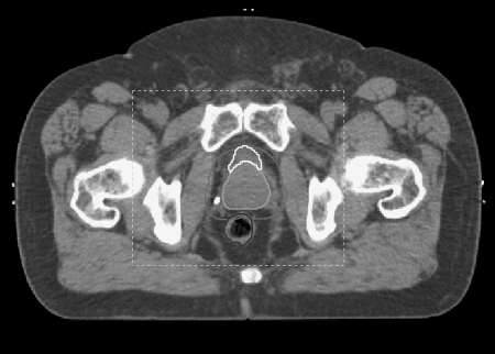
We selected a pair of pelvic CT scans for one patient at random from a database of daily CT scans of a cohort of prostate cancer patients. The scans had 76 slices of 512 × 512 pixels, each 3.00 × 0.922 × 0.922 mm in size. The two scans were deformably registered via an in-house DIR process based on parametric modeling of the DVF with B-splines. The computational details of this algorithm have been reported previously.¹³ One feature of the registration algorithm is the ability to define a limited region of interest (ROI) in the target image, within which the registration is computed. This allows one to focus on key anatomy and obtain the highest spatial resolution for a prescribed number of B-spline control points. However, if one varies the ROI, then the DVF will vary as well. This is one source of uncertainty in DIR. To expose this component of uncertainty we created a set of 50 different ROIs by defining an initial ROI encompassing 200 × 170 × 40 voxels and then randomly varying its position and dimensions by up to 10 voxels in each direction. Figure 1 shows a representative slice of the target image, with the registration region of interest indicated by the dashed rectangle. Each ROI was used to deformably register the two CTs. This gave us 50 different DVFs. We determined the volume of overlap for the 50 ROIs, calculated the mean DVF there, and subtracted it from the individual DVFs to obtain a set of 50 DVF error maps within the overlap volume. This became our training set. Approximately, 95% of the mean DVF vectors were less than 4.0 mm in length. We observed that the individual DVFs within the overall ROI fluctuated with a 0.38 mm root mean square (RMS) deviation around the mean DVF. Approximately 95% of the errors were less than 0.8 mm, but there was a long tail of errors of greater than 1 mm. In proportion to the DVF vector magnitudes, the relative (i.e., normalized) RMS fluctuation was

$$\mathrm{nRMS}={[\sum _i{e}_i^2/\sum _i{(V_i-m)}^2]}^{1/2}=19\%$$ (1)

where V_i is the ith DVF vector magnitude, e_i is the ith displacement vector error, and m is the mean of all the displacement vectors V_i.

Figure 1.

A representative slice of the male pelvic CT showing the contoured organs for computing the dose plan and the registration region of interest (box).

Principal component analysis of the training set

Suppose that we have N DVF error maps, each of which has M voxels. We arrange them into N feature vectors {v_i}, i = 1, … N, each with M components (indexed j = 1, …, M), to form the training set. We expand each feature vector on an orthonormal basis {u_k} as follows:

$$\mathbf{v}={}^M{\displaystyle \sum _k{p}_k{\mathbf{u}}_k}$$ (2)

There are a maximum of M basis vectors indexed by k, each of dimension M. We want to find the basis for which the expansion coefficients p_k are maximally uncorrelated.¹⁴ This basis is made up of the so-called principal components of {v_i}.

To find the principal components of {v_i}, we compute the mean 〈v〉 of the feature vectors, subtract it to get v_i − 〈v〉, and arrange the N zero-mean column vectors in the M × N matrix V. The M × M covariance matrix of the training data is then

$$C=(1/N)\sum _i({\mathbf{v}}_i-〈\mathbf{v}〉){({\mathbf{v}}_i-〈\mathbf{v}〉)}^T=(1/N)V{V}^T$$ (3)

The M principal components u_k (i.e., eigenvectors) of the training set and their associated eigenvalues λ_k are solutions of the eigenvalue problem

$$C{\mathbf{u}}_k=(1/N)V{V}^T{\mathbf{u}}_k={\lambda }_k{\mathbf{u}}_k$$ (4)

We collect the eigenvectors u_k into an M × M matrix U of M column vectors.

Principal components analysis uses the M orthonormal eigenvectors u_k (the principal components) to rotate the zero-mean feature vectors v_i − 〈v〉 into a new set of (zero-mean) vectors p_i

$$U^T({\mathbf{v}}_i-〈\mathbf{v}〉)={\mathbf{p}}_i$$ (5)

In this discussion, we will call the p_i the principal coefficient vectors. Each of the M elements p_ki of p_i is maximally uncorrelated with all the other elements and has an associated eigenvalue λ_k that equals the variance of that component over the set of N feature vectors.¹⁴ The computational process arranges the eigenvalues and eigenvectors in order of decreasing variance. If the individual elements (voxels) in the feature vectors are strongly correlated, then the eigenvalue spectrum will fall off rapidly and there will be only a few dominant eigenmodes. If the voxels are completely uncorrelated (as with white noise) then the eigenvalue spectrum will be flat and Eq. 4 will have many degenerate solutions for the eigenvectors, indicating that the principal component basis has no preferred directionality. Therefore, PCA is a powerful test of correlations among the elements of a data vector.

Estimating the PDFs of the principal coefficients and sampling from them to construct a sample error map

The ensemble of the kth principal coefficients p_{k(i = 1,…N)} of the N rotated error feature vectors will be distributed according to a probability density function P_k(p). If the training set used for PCA has a Gaussian distribution around its mean, then it can be completely described by its covariance and the principal coefficients and their associated PDFs P_k(p) are stochastically independent. If the data are not Gaussian, or have multiple Gaussian modes, then although PCA will maximally decorrelate the training data, the principal coefficients will not necessarily be completely independent. For our sampling method, we assume that they are stochastically independent. However we also assume that we do not know the shape of P_k but, as noted above, its mean squared value (variance) should be λ_k. Also, we have only a sparse sampling of it from our training set of N DVF maps. Therefore we use kernel density estimation¹⁵ to build continuous PDFs from the N examples of p_ki (Kernel density estimation is a very useful nonparametric way to estimate the continuous parent PDF from a small ensemble of samples when one doesn’t know its shape a priori.)

Using a Gaussian kernel, the Parzen¹⁵ estimation of the PDF for {p_{k(i = 1,…N)}}k = 1, … M, is

$$P_k\left(p\right)=(1/\sqrt{2\pi })(1/\sigma ){(1/N)}^N\sum _i\exp [-{(p_{\mathit{ki}}-p)}^2/2{\sigma }^2]$$ (6)

where σ is a smoothing parameter. Determining the optimal smoothing parameter (also referred to as the bandwidth) for kernel density estimation is in general a difficult problem, but for a Gaussian kernel and PDFs that are approximately unimodal and symmetric about their mean, a good estimate is^{16, 17, 18}

$$\sigma ={\left[d/\left(\left(d+2\right)N\right)\right]}^{\text{1/}(d+4)}{\left(\text{SD}\right)}_{\text{data}}$$ (7)

where (SD)_data is the standard deviation of the data and d is the dimensionality of the data space. For a univariate distribution, this equals

$$\sigma =[1.06/N^{1/5}]{\left(\mathrm{SD}\right)}_{\mathrm{data}}$$ (8)

To make a sample synthetic DVF error map, we randomly pick a principal coefficient π_k from each P_k(p) via importance sampling, refer back to the PCA expansion in Eq. 2 and make a sample error feature vector according to

$$e={}^M{\displaystyle \sum _k{\pi }_k{\mathbf{u}}_k}$$ (9)

which we then reconfigure as a 3D error map.

Validating the error sampling procedure

There are several practical aspects of PCA that can affect the validity and accuracy of our DVF error modeling and sampling procedure. To begin, the feature vectors in the PCA training set will have a large number of components, whereas our training set of measured DVF errors for training will be comparatively small. Therefore the dimension M of the covariance matrix will potentially be (much) larger than the number N of sample feature vectors used to compute the covariance. This is the so-called “curse of dimensionality” that afflicts many pattern recognition problems. It results in a sparse covariance matrix where many of the points in the principal component space are unrepresented by sample data. While there is a standard method to compute the eigenvectors and eigenvalues of the covariance matrix under these conditions (see, for example, page 569 of Bishop¹⁹) one can ask whether there are enough examples of training data to adequately constrain the solution. One common criterion for adequate data is to have more sample vectors than there are significant eigenmodes in the data. Another test is whether the eigenvalue spectrum changes when the number of training examples changes. We tested our method for sufficient training data by reducing the number of training examples from 50 to 10 while monitoring the eigenvalue spectrum for changes.

A second concern is how well can the PCA-based sampling procedure simulate arbitrary error distributions? If the parent data set used for the PCA has a Gaussian distribution around its mean, then it can be completely described by its covariance and the principal coefficients are stochastically independent. This would validate our assumption that the random samples we draw from the PDFs of the coefficients are statistically independent and we can ignore cross-correlations among them. However, if the data are not Gaussian, or have multiple Gaussian modes, then although PCA decorrelates the training data, the principal coefficients are not necessarily completely independent. This might bias our sampling process.

To validate our method we created a training set of 50 error maps and a validation set of 50 different maps. From the training set, we constructed PDFs of the principal error coefficients as described above, drew 50 random samples from our PDFs and constructed 50 synthetic maps of the DVF uncertainties. We then compared the PCA eigenvalue spectrum of the synthetic map set to the spectrum of the validation set. We also compared the individual PDFs of the principal coefficients of the validation set and the synthetic set using the Kolmogorov-Smirnov test. The purpose of this was to see if the PCA of the error data, combined with our kernel-based PDF estimation and sampling process, produced an ensemble of synthetic error maps that was indistinguishable from the real maps.

Modeling dose mapping uncertainties

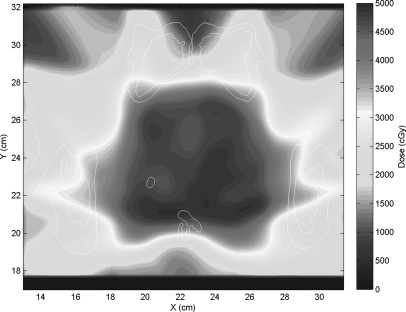
Having validated our error sampling method, we used it to produce an ensemble of mapped doses. We did this by calculating a clinical dose plan on one of our two pelvic CTs (see Figs. 12). The plan was then applied to the other CT and the calculated dose was mapped back to the planning CT using 50 DVFs created via the B-spline deformable registration described above, each perturbed by a different error map based on the variable ROIs and created by our DIR error sampling process. The 50 mapped dose distributions were averaged, and then, the difference of each dose map from the average was computed. This revealed the patterns of dose mapping uncertainty arising from the DVF uncertainty.

Figure 2.

The prostate dose plan calculated on the patient’s first CT.

To demonstrate the significance of spatial coherence in the error maps, we repeated the dose mapping trials using error maps in which the DVF error varied voxel-by-voxel as white noise with a variance equal to that of the spatially-correlated uncertainties.

RESULTS

Deformable image registration uncertainties due to ROI choice

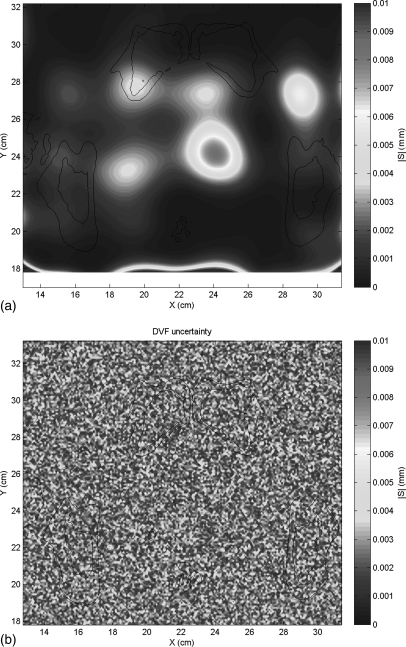
Figure 3a shows a representative example from the training set of DIR error maps due to the variable ROI. Figure 3b shows a random white noise error map with the same RMS error. The spatial distribution of DIR errors is smooth and homogeneous over large areas, in contrast to the random spatial distribution of errors.

Figure 3.

(a) An example map of the DVF error arising from the variable registration region of interest and (b) a random white noise error map with the same RMS error.

PCA of the ROI error maps

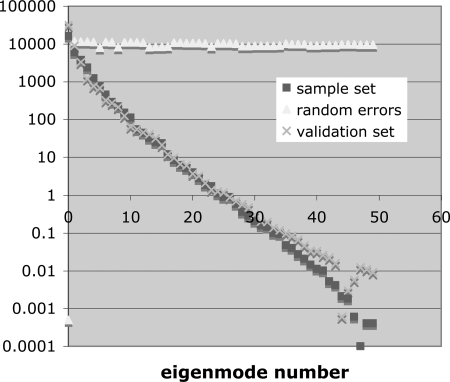
Figure 4 shows the eigenvalue spectra for our validation set of 50 error maps and for our set of 50 synthetically sampled maps, together with the eigenvalue spectrum for 50 maps of random error. As expected, the ensemble of random error maps has a flat eigenvalue spectrum, consistent with the absence of any cross-correlation between pixels (i.e., the covariance matrix is diagonal), while the spectrum for the actual error maps falls off steeply, indicating the presence of strong cross-correlations among the pixels.

Figure 4.

The PCA eigenvalue spectra for the validation set of 50 spatially-correlated error maps, the synthetic sample set of 50 correlated error maps, and a set of 50 random uncorrelated error maps with the same RMS error.

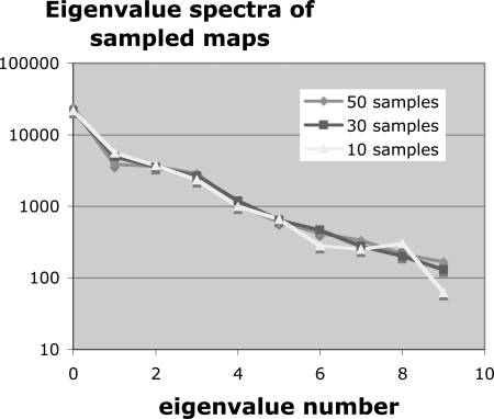
To test the importance of sample size N, we calculated the eigenvalue spectrum for subsets of N = 10, 30, and 50 samples. Figure 5 shows these spectra. There is no appreciable difference among them. We also note from Fig. 4 that more than 99% of the variance is in the first ten eigenmodes, which suggests that ten or more training examples should be sufficient. We conclude that we have sufficient training data in our 50 samples.

Figure 5.

PCA eigenvalue spectrum versus number of samples in the training set.

Making and validating sample error maps

From the PDFs [Eq. 6] of the principal coefficients in Eq. 2, we drew independent samples π_k and constructed 50 synthetic error maps according to Eq. 9. The PCA eigenvalue spectra of the validation and synthetic sets of error maps are shown in Fig. 4. These spectra are essentially identical. The Kolmogorov-Smirnov test comparing the PDF of each of the 50 principal coefficients of the validation set and the synthetic set returned p-values ranging from 0.20 to 1.0 (with 39 of 50 above 0.90). Here, the p-value is the likelihood that the two data sets were drawn from the same parent distribution. By way of comparison, the same test applied to the validation set and the training set returned p-values ranging from 0.43 to 1.0 (with 42 of 50 values above 0.90). These tests indicate that the synthetic sample error maps are accurate emulations of the actual error maps, which validates our sampling process.

For our demonstration purposes, we have used a single pair of pelvic CTs to derive deformable registration error maps, model and sample them, and use the samples to expose the effects of registration error on dose mapping between the two CTs. However, to ensure that the error modeling and sampling process is generalizable to error maps obtained from a more general set of deformable registration results, we repeated the sampling validation tests with error maps derived from a variable region of interest applied to registrations of three pairs of pelvic CT studies for three different patients. Each pair of CT registrations contributed 20 training examples and 20 validation examples, for a total of 120 training and validation maps and 60 sample error maps. As before, the eigenvalue spectra for the validation and sample sets were essentially identical and the Kolmogorov-Smirnov test showed that the distributions of principal coefficients were indistinguishable.

Mapped dose uncertainty due to the DVF uncertainty associated with ROI choice

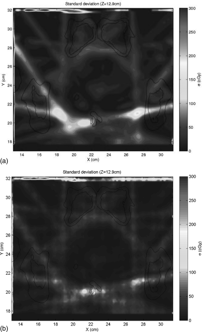
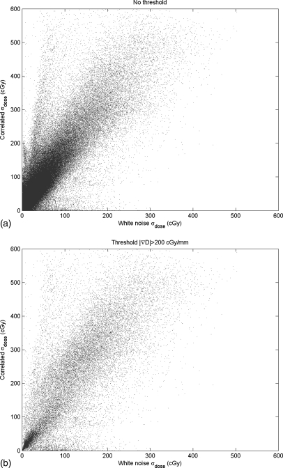
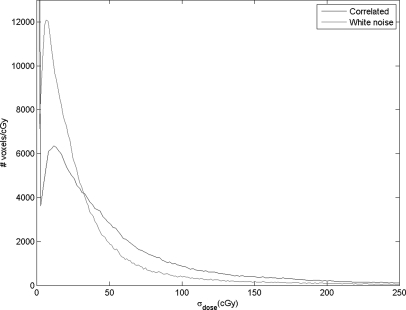
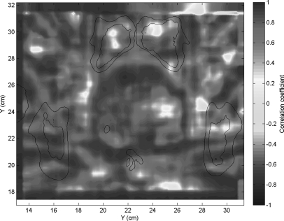
Figure 2 shows the calculated dose plan on the delivery CT. This dose was mapped back to the planning CT using DIR of the two CTs, with the resulting DVF perturbed by 50 sampled DIR error maps. Figure 6a shows the voxel-by-voxel variance of the dose mapping due to the spatially-correlated uncertainties caused by the ROI variability, as estimated by our error sampling procedure. Figure 6b shows the variance in dose mapping caused by a random white noise pattern of DIR uncertainty with the same variance as the correlated uncertainties. We note that the errors in dose mapping for both patterns of DIR error are in general larger in the regions of highest dose gradient, but the correlation between dose gradient and dose mapping error is weak, in accordance with previously reported results.^{5, 11} In particular, there are three bright islands of mapping error apparent in Fig. 6a that are not nearly as prominent in Fig. 6b. The dose mapping errors due to correlated DIR errors are noticeably larger than those due to random errors. This is seen in the scatter plot of the dose mapping error due to correlated DIR uncertainty versus that due to random DIR error [Fig. 7a], which has a slope of about 1.75, with a subset of dose mapping errors that are substantially larger for the correlated DIR errors. If we filter this scatter plot to select the dose mapping errors in the regions of high dose gradient [Fig. 7b], the trend persists. The histograms of the frequencies of correlated versus random mapping errors (Fig. 8) also show that spatial correlations in DIR uncertainty tend to increase the resulting dose mapping error. However, the local correlation coefficient between mapping errors due to ROI uncertainty and random DIR error, seen in Fig. 9, shows that the relative magnitude of the mapping error due to spatially-correlated versus uncorrelated DIR errors is not spatially uniform.

Figure 6.

The dose mapping errors due to (a) the PCA model of DIR error for spatially-correlated errors and (b) random spatial errors with the same RMS magnitude.

Figure 7.

The correlation between the dose mapping errors due to correlated DIR errors and those due to random spatial errors, (a) from the entire dose distribution and (b) selected from the regions of higher dose gradient.

Figure 8.

The frequency distributions of dose mapping errors for our two models of DIR uncertainty.

Figure 9.

The local spatial correlation between the dose mapping error due to spatially-coherent DIR errors and that due to random white noise DIR errors.

DISCUSSION

In this study, we have developed a method to test the effects of DIR uncertainty on daily dose mapping for external beam radiation therapy. We first developed a statistical sampling model for DIR errors that correctly recreates DVF uncertainties that have strong spatial correlations. The DIR uncertainty model was then used in a Monte Carlo type manner to propagate DIR errors through the dose mapping process in order to simulate the resulting dose errors. We then compared the results with a considerably simpler random DVF uncertainty model that made no assumptions about spatial error correlation. We observed that the naïve random error model underestimates the dose mapping error. Furthermore, the spatial patterns of dose mapping errors for the two models are distinctly different. The significance of these differences must be judged with respect to the accuracy needed in the mapped and accumulated dose. We conclude that the spatial coherence of DVF errors can influence the dose mapping error and therefore should not be ignored.

For a typical intensity-based DIR algorithm, the DVF uncertainty will generally be the smallest at organ and other feature boundaries, and the largest in areas of uniform gray-scale intensity. We see this in Fig. 3, where the largest DVF errors occur well inside the contour of the prostate. On the other hand, the largest dose mapping uncertainties will generally be in the regions of high dose gradient, as we see in Fig. 6. This raises the following interesting point as IGRT moves toward more precise daily plans with smaller margins, and potentially to the point where organ and tumor subvolumes are targeted for boosts. The accuracy of the DVF error model will be most important when summing doses in plans with high dose gradients in anatomical regions of high registration uncertainty. This will be conspicuously the case if, e.g., the PTV is a subvolume of the prostate targeted for a boost. If the regions of high DVF accuracy roughly coincide with regions of high dose gradient (i.e., right at the organ boundary), then the estimated dose mapping errors will likely be fairly insensitive to the details of the DVF error estimation model.

Just as with error sampling via the bootstrap process, our error modeling and sampling method requires a training set that is made up of multiple individual instances of measured DIR errors throughout a registered region of interest. If the DIR error measurements have already been reduced to means and variances, as is often the case in reported studies of deformable registration accuracy, then the information needed for the PCA analysis has been lost. Measuring DIR errors is a complicated subject all of its own. One can expect the error maps to depend on the anatomy present in the registered region of interest, which will depend in turn on the individual patient characteristics. It can be problematic to combine DIR error studies from a population of subjects into a generic training set for our sampling method. We will take up the problem of developing the DVF error training set in a follow-on study.

SUMMARY

We have developed a statistical sampling procedure that can model complex DIR error distributions and shown that this procedure can be used to study their impact on dose mapping. Using such a model instead of making simplified assumptions about the DIR errors will result in a more accurate and nuanced estimate of dose mapping uncertainty. The significance of this improvement, though, will depend on expectations and requirements for dose mapping accuracy.

References

- Birkner M. et al. , “Adapting inverse planning to patient and organ geometrical variation: Algorithm and implementation,” Med. Phys. 30, 2822–2831 (2003). 10.1118/1.1610751 [DOI] [PubMed] [Google Scholar]
- Zhang P., Hugo G. D., and Yan D., “Planning study comparison of real-time target tracking and four-dimensional inverse planning for managing patient respiratory motion,” Int. J. Radiat. Oncol., Biol., Phys, 72(4), 1221–1227 (2008). 10.1016/j.ijrobp.2008.07.025 [DOI] [PubMed] [Google Scholar]
- Brock K. K. et al. , “Results of a multi-institution deformable registration accuracy study (MIDRAS),” Int. J. Radiat. Oncol., Biol., Phys. 76(2), 583–596 (2010). 10.1016/j.ijrobp.2009.06.031 [DOI] [PubMed] [Google Scholar]
- Kashani R. et al. , “Objective assessment of deformable image registration in radiotherapy: A multi-institution study,” Med. Phys. 35(12), 5944–5953 (2008). 10.1118/1.3013563 [DOI] [PMC free article] [PubMed] [Google Scholar]
- Saleh-Sayha N. K., Weiss E., Salguero F. J., and Siebers J. V., “A distance to dose difference tool for estimating the required spatial accuracy of a displacement vector field,” Med. Phys. 38(5), 2318–2323 (2011). 10.1118/1.3572228 [DOI] [PMC free article] [PubMed] [Google Scholar]
- Yan C. et al. , “A pseudoinverse deformation vector field generator and its applications,” Med. Phys. 37(3), 1117–1128 (2010). 10.1118/1.3301594 [DOI] [PMC free article] [PubMed] [Google Scholar]
- Zhang G. G. et al. , “Dose mapping: Validation in 4D dosimetry with measurements and application in radiotherapy follow-up evaluation,” Comput. Methods Programs Biomed. 90(1), 25–37 (2008). 10.1026/j.cmpb.2007.11.015 [DOI] [PubMed] [Google Scholar]
- Huang T. C. et al. , “Four-dimensional dosimetry validation and study in lung radiotherapy using deformable image registration and Monte Carlo techniques,” Radiat. Oncol. 5(45), (2010). [DOI] [PMC free article] [PubMed] [Google Scholar]
- Zhong H. and Siebers J. F., “Monte Carlo dose mapping on deforming anatomy,” Phys. Med. Biol. 54(19), 5815–5830 (2009). 10.1088/0031-9155/54/19/010 [DOI] [PMC free article] [PubMed] [Google Scholar]
- Hub M., Kessler M. L., and Karger C. P., “A stochastic approach to estimate the uncertainty involved in B-spline image registration,” IEEE Trans. Med. Imaging 28(11), 1708–1716 (2009). 10.1109/TMI.2009.2021063 [DOI] [PubMed] [Google Scholar]
- Salguero F. J., Saleh-Sayah N. K., Yan C., and Siebers J. V., “Estimation of three-dimensional intrinsic dosimetric uncertainties resulting from using deformable image registration for dose mapping,” Med. Phys. 38(1), 343–353 (2011). 10.1118/1.3528201 [DOI] [PMC free article] [PubMed] [Google Scholar]
- Vaman C., Staub D., Williamson J., and Murphy M. J., “A method to map errors in the deformable registration of 4DCT images,” Med. Phys. 37(11), 5765–5776 (2010). 10.1118/1.3488983 [DOI] [PMC free article] [PubMed] [Google Scholar]
- Murphy M. J., Wei Z., Fatyga M., Williamson J., Anscher M., Wallace T., and Weiss E., “How does CT image noise affect 3D deformable image registration for image-guided radiotherapy planning?,” Med. Phys. 35(3), 1145–1153 (2008). 10.1118/1.2837292 [DOI] [PubMed] [Google Scholar]
- Kittler J. and Young P. C., “A new approach to feature selection based on the Karhunen-Loeve expansion,” Pattern Recogn. 5, 335–352 (1973). 10.1016/0031-3203(73)90025-3 [DOI] [Google Scholar]
- Parzen E., “On estimation of a probability density function and mode,” Ann. Math. Stat. 33, 1065–1076 (1962). 10.1214/aoms/1177704472 [DOI] [Google Scholar]
- Silverman B. W., “Density Estimation for Statistics and Data Analysis,” Monographs on Statistics and Applied Probability (Chapman and Hall, London, 1986). [Google Scholar]
- Scott D. W., “Multivariate Density Estimation: Theory, Practice, and Visualization” (John Wiley, New York, 1992).
- Bowman A. W. and Azzalini A., Applied Smoothing Techniques for Data Analysis (Oxford University Press, London, 1997). [Google Scholar]
- Bishop C. M., Pattern Recognition and Machine Learning (Springer, New York, 2006). [Google Scholar]