Abstract
Several popular classification algorithms used to segment magnetic resonance brain images assume that the image intensities, or log-transformed intensities, satisfy a finite Gaussian mixture model. In these methods, the parameters of the mixture model are estimated and the posterior probabilities for each tissue class are used directly as soft segmentations or combined to form a hard segmentation. It is suggested and shown in this paper that a Rician mixture model fits the observed data better than a Gaussian model. Accordingly, a Rician mixture model is formulated and used within an expectation maximization (EM) framework to yield a new tissue classification algorithm called RiCE (Rician Classifier using EM). It is shown using both simulated and real data that RiCE yields comparable or better performance to that of algorithms based on the finite Gaussian mixture model. As well, we show that RiCE yields more consistent segmentation results when used on images of the same individual acquired with different T1-weighted pulse sequences. Therefore, RiCE has the potential to stabilize segmentation results in brain studies involving heterogeneous acquisition sources as is typically found in both multi-center and longitudinal studies.
Keywords: Medical Image segmentation, Tissue Classification, Rician Distribution, Biomedical Imaging
1. Introduction
Various automated segmentation techniques have been proposed to segment brain tissues—typically cerebrospinal fluid (CSF), gray matter (GM) and white matter (WM)— in magnetic resonance (MR) images. Accurate and reliable tissue segmentation is extremely important to the neuroscience community because it is a key step in nearly every image-based study of the brain in health and disease (Resnick et al., 2003; Querbes et al., 2009; Raz et al., 2003). Manual segmentation by experts is still considered to be the gold standard in brain quantification though automated or semi-automated segmentation is acceptable for large-scale studies in which the image acquisition parameters are identical and manual segmentation is impractical (Tu et al., 2007).
Fully automated brain tissue segmentation algorithms can be sensitive to noise, partial volume e ects, acquisition protocols, scanner differences, and imaging artifacts such as intensity inhomogeneities, zippers, and ringing. Techniques have been proposed to address all of these limitations and have been very successful in large part. Most algorithms incorporate spatial smoothness to reduce isolated misclassification due to noise and local artifacts (cf. (Li, 1995; Leemput et al., 1999)). Intensity inhomogeneities are either estimated in preprocessing (e.g. (Sled et al., 1998; Chang and Fitzpatrick, 1992; Vovk et al., 2004)) or incorporated within the classification algorithm itself (e.g. (Pham and Prince, 1999; Pham, 2001; Styner et al., 2000)). Incorporation of statistical atlases (cf. (Woolrich et al., 2009; Prastawa et al., 2004)) and control of topology (Bazin and Pham, 2007) have been used to reduce misclassification error through incorporation of prior knowledge. The partial volume e ect is typically addressed by producing a soft classification, i.e. one that provides membership functions or posterior densities associated with each tissue class (Leemput et al., 2003; Choi et al., 1991; Noe and Gee, 2002). The e ect can also be addressed by super-resolution methods (Rousseau, 2008; Souza and Senn, 2008), probabilistic models, or topological methods (Bazin and Pham, 2007; Wua and Chung, 2009; Leemput et al., 2009).
Compensation for different acquisition protocols or scanner differences has been particularly problematic for tissue segmentation algorithms (Clark et al., 2006). Approaches to normalize histograms to a common scale have been proposed (Nyul and Udupa, 1999; Han and Fischl, 2007; He et al., 2008), and most recent algorithms use some kind of explicit or implicit intensity normalization preprocessing in practice. Achieving true pulse sequence independence, though, currently requires one to use special pulse sequences (Fischl et al., 2004) that permit compu tation of the underlying tissue parameters to which a segmentation algorithm can be applied (Prince et al., 1995). Though admirable in spirit and quite effective, common practice precludes routine use of special pulse sequences, and modern study designs have typically relied on the use of a multiple scanners or types of scanners or multiple structural acquisition protocols with fixed parameters (Shock et al., 1984; Mueller et al., 2005) in order to yield images whose segmentations can be quantitatively compared within a particular study (Wolz et al., 2010).
Two classes of tissue classification methods have emerged as leading algorithms for MR brain image segmentation: methods (Bezdek et al., 1993; Pham and Prince, 1999; Siyal and Yu, 2005) based on fuzzy c-means (FCM) (Bezdek, 1980) and methods based on a Bayesian framework using a finite Gaussian mixture model assumption (Leemput et al., 2003; Hong et al., 2007; Woolrich et al., 2009; Ashburner and Friston, 2005; Awate et al., 2006). Both approaches have been augmented to account for spatial smoothness (Pham, 2001; Held et al., 1997; Scherrer et al., 2008), most commonly using a Markov random field (MRF) (Li, 1995). At this time, the performances of these methods are very similar “across the board” and the algorithms are widely used in large-scale studies. Yet experience shows that algorithm parameters must be tuned in order to achieve satisfactory results when acquisition parameters change. We suggest in this paper that both classes of algorithms operate with a less accurate model of image intensity and that improving the model can provide improved segmentation and robustness to pulse sequence changes.
The FCM method is not based on an underlying intensity model, though one can tease apart the variational formulation in order to assert its basic assumptions. In its conventional formulation, FCM is a clustering method that associates voxels to all classes in proportion to the value of its computed membership functions. The clusters are uniformly spread around each center intensity, which is also estimated by the algorithm. The so-called “fuzziness parameter” in FCM, roughly speaking, determines how spread out the clusters are from their centroids (Yu et al., 2004; Roy et al., 2008). The basic formulation is not Bayesian, and there is no formula relating the underlying tissue intensities to the observed intensities and there is no explicit noise model. Accommodations have been made to account for clusters that might not have the same size (Cavalcanti and de Carvalho, 2005; Roy et al., 2008; Gustafson and Kessel, 1979), but the added parameters must generally be known in advance and tuned to any given pulse sequence.
The most common Bayesian formulations are based on a finite Gaussian mixture model, in which the conditional probability of the image intensity for a particular tissue type is Gaussian (Leemput et al., 1999). The parameters of the underlying Gaussian conditional probabilities (and often the mixture coeffcients that proportionally weight these densities) are typically estimated using the expectation maximization (EM) algorithm (Dempster et al., 1977). If image smoothness is maintained through the use of an MRF, then the EM algorithm solves a maximum likelihood estimation problem and optimal estimates of both the mixture parameters and the posterior densities are found. The model choice together with the estimation procedure automatically accommodates for clusters that might be of different sizes and relative proportions (if the mixture coeffcients are also estimated). It is logical to assume that the additional flexibility of this model together with the Bayesian optimality would lead to a better result than FCM. However, there are numerous papers that support the contrary opinion.
We are led to question the underlying assumption of a Gaussian model of the intensities in the current Bayesian methods. In conventional MR imaging, the acquired raw data is the underlying signal in “real” (in-phase) and “imaginary” (quadrature phase) channels, each of which is corrupted by additive zero-mean i.i.d. Gaussian noise. The complex image intensities are obtained using the Fourier transform, which preserves the Gaussian nature of the noise in the real and imaginary components of the image intensities (Bernstein et al., 1989). Since the observed image intensities are formed by taking the complex modulus of the real and imaginary parts of the complex image, each image voxel becomes a Rician random variable (Gudbjartsson and Patz, 1995; Henkelman, 1985). See Sec. 2 for more details.
The underlying signal values are generally different at each voxel because of biological variability. Therefore, the probability distribution that describes the collection of all voxels taken together is a Rician mixture model in which there is a different conditional Rician probability density function for each underlying signal value. By noting that within each tissue class the underlying signal intensities are close in value, this rich mixture model can be approximated by one that has only three conditional Rician probability densities, one for each tissue class. When the underlying signal values are large relative to the noise, it is known that a Rician distribution can be approximated by a Gaussian distribution (Sijbers et al., 1998). But since this approximation becomes less accurate with smaller underlying signal values, we can expect the greatest impact of using this Rician mixture model versus a Gaussian mixture model to be in the tissue classes having the smallest underlying signal values.
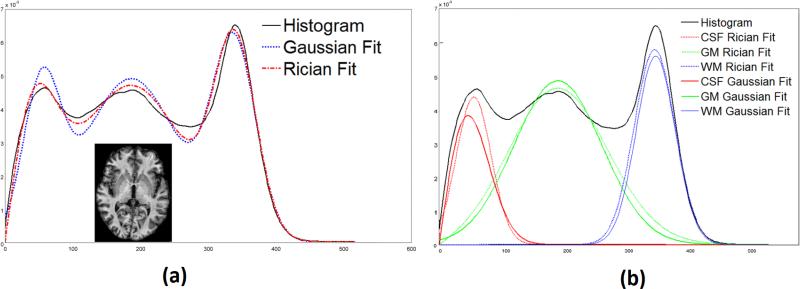
To illustrate this point, in Fig. 1(a) we show the smoothed histogram of intensities in an inhomogeneity corrected (Sled et al., 1998) MPRAGE (Magnetization Prepared Rapid Gradient Echo) image together with two fitted histograms, one using a mixture of Gaussians (blue) and one using a mixture of Ricians (red). It is observed that the Rician fit is better, an observation that can be quantitatively verified by noting that the Kullback-Leibler (KL) distances (Kullback and Leibler, 1951) between the image histogram and the Gaussian fit is 0.0418 and between the image histogram and the Rician fit is 0.0097. In Fig. 1(b), the fits of the individual class conditional probabilities derived from the Gaussian (blue) and Rician (red) fitting process. It is observed that the CSF densities show the most difference, which is to be expected since these intensities are the lowest. The WM densities are most similar, which makes sense since these tissues have the highest intensities in this T1-weighted pulse sequence, and are likely to be well approximated by a Gaussian as a result.
Figure 1.
(a) The histogram (solid black) of an inhomogeneity corrected (Sled et al., 1998) MPRAGE image (shown inset), overlapped with a Gaussian (dotted blue) and Rician (dashed dot) fitting. The KL distance (Kullback and Leibler, 1951) between the histogram and Gaussian fit is 0.0418, while it is 0.0097 between the histogram and the Rician fit. (b) CSF, GM, WM distributions as obtained from the Rician (dot) and Gaussian (solid colored) fit. The histograms are smoothed with a Gaussian kernel of standard deviation of 3.0.
In this paper, we propose a brain image tissue segmentation algorithm based on an underlying finite Rician mixture model, which we call Rician Classifier using EM (RiCE). We primarily focus on the difference between Rician and Gaussian models of the tissue intensities. Consequently, we do not include any bias-field correction in our method, instead, we pre-process all the data using a non-parametric inhomogeneity correction method (N3) (Sled et al., 1998). Although the inhomogeneities in different MR sequences can depend on the sequence itself, N3 has been shown to work well on different sequences (Manjon et al., 2007; Mangin, 2000). In order to include smoothness on the resulting segmentation, the algorithm includes an MRF model. This fully automatic algorithm does not require parameter choices, relying instead on the assumption that cluster intensity distributions will be Rician regardless of the pulse sequence. The main contribution of this work is to improve segmentation consistency between different pulse sequences having T1-weighted (T1w) contrast. We compare our method with a Gaussian intensity model approach, SPM (spm segment function) (Ash-burner and Friston, 2000, 2005; Chard et al., 2002), a Gaussian model approach on log-transformed intensities, FAST (Woolrich et al., 2009) and two FCM based approaches, Freesurfer (Dale et al., 1999) (mri_ms_EM function) and FANTASM (Pham, 2001).
We outline our assumptions on noise models and EM are explained in Sec. 2 and the algorithm is described in Sec. 3. Validations on simulated and real data are presented in Sec. 4.1 and Sec. 4.2, respectively. Then we show the improvement in segmentation consistency of the Rician model over a comparable Gaussian model in Sec. 5 and the comparison of our method with other state of the art methods in Sec. 6.
2. Background
2.1. Noise Estimation
Magnitude images are most commonly used in MRI. They are acquired in two steps. Complex data is acquired in separate in-phase and quadrature phase channels. We assume that each channel is corrupted with uncorrelated additive Gaussian noise, having zero mean and the same variances (Gudbjartsson and Patz, 1995; Bernstein et al., 1989; Henkelman, 1985). Then real and imaginary images are reconstructed from the complex data by inverse Fourier transform. The inverse Fourier transform, being linear and orthogonal, preserves the Gaussian nature of the noise and the noise between the real and imaginary images remain zero mean and uncorrelated. Define AR and AI to be the true noise-free real and imaginary reconstructed images. They are corrupted by additive zero-mean independent Gaussian noise with the same variance σ2. Thus the intensity image y is the magnitude of the complex image AR + jAI, and can be shown to have the following Rician distribution (Rice, 1954).
| (1) |
where and Ip is the modified pth order Bessel function of the first kind.
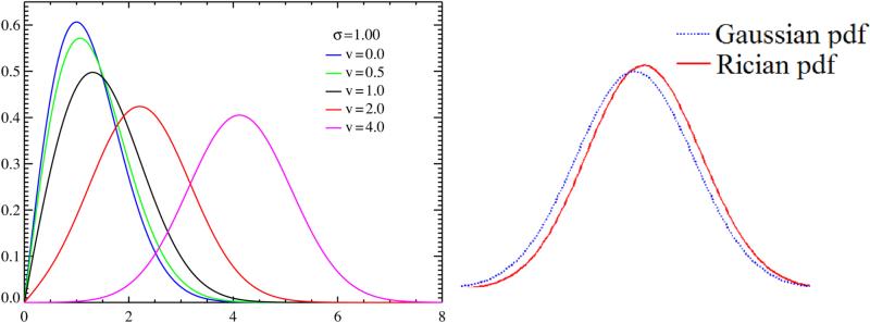
Fig. 2(a) shows that the Rician PDF is quite different from a Gaussian for low SNR, where SNR is defined as . For higher SNR (> 2), it can be shown that the Rician distribution asymptotically approaches a Gaussian distribution with mean and variance σ2 (Sijbers et al., 1998). Fig. 2(b) shows a Rician PDF with SNR = 2, with the corresponding asymptotic Gaussian mean and variance σ2. Clearly, the Gaussian PDF is biased for high SNR (=2) and any estimator based on a Gaussian assumption will also be biased. For example, the CSF having a low SNR follows the Rician more closely than a Gaussian (Fig. 1(a)). Thus a Gaussian approximation of the PDF will lead to a biased segmentation and a Rician estimation of the PDF will be more appropriate. We describe in the next section how such a Rician estimation approach can be formulated and carried out using the EM algorithm.
Figure 2.
(a) Rician distribution of y (Sec. 2.1) for different values of v (Wikipedia, 2011), (b) Rician PDF (red) overlapped with the corresponding Gaussian one (blue) for SNR = 2. Clearly, Gaussian approximation of the actual Rician PDF is biased.
2.2. Expectation Maximization
We want to classify a brain MR image into three major tissue classes, CSF, GM, and WM. Given a voxel intensity yi,j ∈ Ω, Ω being the image domain, define zjk as the indicator function of the jth voxel belonging to the kth class, k = 1, . . . , K. In our case, K = 3, for the three classes. Thus, zjk is equivalent to the hidden underlying true segmentation of the tissues. Also define the Rician parameters for the kth class to be {vk,σk}.
Let the unknown prior probabilities of observing yj from the kth class be πjk. Now a finite mixture model representation of the likelihood of observing yj is given by
| (2) |
where zj = [zj1, zj2, . . . , zjk] is a 1 × K vector of indicator functions. The parameter collection Θ can be defined as
| (3) |
Here, the πjk's can be treated as unknown parameters, but the number of such parameters is still large (K × |Ω| Later, we will parametrize πjk using an MRF approach and redefine Θ so that the number of unknown parameters is smaller.
The segmentation problem now becomes an estimation problem, where the estimates of the underlying segmentation zj's are calculated from the observed intensities yj. The segmentation can be computed if Θ is known, while is known only when zjk's are known. This naturally leads to the use of the EM algorithm to find the maximum likelihood (ML) estimate of the parameters –
| (4) |
The EM algorithm iteratively estimates the underlying true segmentation zjk based on the current estimate of Θ, and then updates Θ based on the estimate of zjk. This can be described as a two step process :
- E Step : To find new update Θ(m+1) at the mth iteration, we compute,
- M Step : Find new estimation Θ(m+1) based on the previous estimation of parameters Θ(m) using the following equation,
where is the true underlying segmentation of the whole image.
The algorithm terminates if the difference between log-likelihoods of successive iterations drops below a certain threshold. It has been shown that the EM algorithm is guaranteed to increase the likelihood, but the final convergence depends heavily upon its initialization. If the algorithm is not initialized near the true maximum, it may find a local optimum, so the EM is often initialized using some prior information about Θ.
3. Method
3.1. A Finite Mixture Model using Ricians
We now develop an EM classification algorithm for the Rician mixture model. The log-likelihood of Eqn. 2 is extended to include random noise removal by introducing an MRF on the underlying segmentation zjk. The total log-likelihood after these modifications is given by,
| (5) |
The unknown prior probabilities πjk in Eqn. 2 are replaced by a spatially varying function fMRF(zjk|zNj, Θ) following the model described in (Nikou et al., 2007). In the following sections, we will explain each of the terms and modifications added in Eqn. 5. So far, it is evident that {vk, σk} should be estimated, so they are included in Θ. We will add more parameters to Θ as we explain fMRF in Sec. 3.2.
3.2. MRF on the underlying segmentation
Biologically, the underlying segmentation should be locally smooth. The local smoothness is often captured by introducing an MRF on the segmentation (Leemput et al., 2003; Li, 1995), which is essentially a smoothness criteria on the prior probabilities πjk. No spatial relationship was imposed on them in Eqn. 2 and they are assumed to be unknown parameters. Under the MRF assumption, these probabilities depend on the segmentation of the neighborhood voxels. Defining zNj as the underlying segmentation of a neighborhood Nj of the jth voxel, πjk in Eqn. 2 is changed to a spatially varying prior fMRF(zjk|zNj Θ), which depends on the segmentation zNj of the neighborhood Nj.
The exact structure of fMRF depends on the smoothness assumptions of . The Hammersley-Clifford theorem (Besag, 1974) states that for the function fMRF to be a Markov Random Field, it must be of the form,
| (6) |
where U(·|Θ), called the Gibbs potential, is usually a sum of functions of the neighborhoods of each voxel and M is a normalizing constant. The Ising model and the Potts model (Potts, 1952) are two common examples of the Gibbs Potential, which have been successfully used in previous brain tissue segmentation methods (Leemput et al., 1999; Zhang et al., 2001). Usually the most general representations of these models contain a few “interaction coeffcients” (Li, 2001) that are diffcult to estimate. A computationally simpler enhancement to these models has been suggested in (Nikou et al., 2007), where U is taken as a sum of Gaussian functions (Sanjay-Gopal and Herbert, 1998). We follow this idea and define the MRF as,
| (7) |
where is a weighing function. From this Gibbs potential, a natural choice of fMRF(zjk|zNj, Θ) is
| (8) |
is a normalizing constant so as to make . The assumption behind such an MRF is that without any prior knowledge on the smoothness of the underlying segmentations , zjk is assumed to be Gaussian distributed with mean and variance . This formulation assures that the spatial prior fMRF is high if and only if segmentation of the jth voxel is the same as the segmentation of its neighborhood. It is also possible to estimate the variances by EM. Thus the parameter collection Θ becomes,
| (9) |
Now that we have defined Θ and fMRF from Eqn. 5, the maximum likelihood estimate of Θ is described in the next section.
3.3. Classification Algorithm
To estimate the parameters given in Eqn. 9, we use the EM algorithm to maximize the log-likelihood from Eqn. 5. The E step requires computation of E(zjk|yj, Θ). Using the fact that zjk is a binary variable with zjk ∈ {0, 1} , it can be shown that P(zjk = 1|yj, Θ) = E(zjk|yj, Θ). Thus the conditional probability is also the conditional expectation. Define as the conditional expectation at the mth iteration of the EM algorithm. Then using the mean-field approach (Zhang, 1992; Li, 1995) to approximate the true conditional MRF by its estimate, we obtain,
| (10) |
| (11) |
where zjk is replaced by its current conditional expectation .
The M step requires estimation of Θ given the current segmentation . The update equations are given by,
| (12) |
| (13) |
| (14) |
Here, N is the number of voxels in the image domain and,
Eqn. 12 to Eqn. 14 are solved by a coordinate descent method to find each of , and . We continue iterating through the EM algorithm until the increases in log-likelihood of successive iterations are below a threshold. The derivations of Eqns. 11–14 are provided in the Appendix.
The algorithm is executed in the following way. The parameters {vk, σk,βk} are first initialized by a k-means algorithm, then the estimates are fed to a Gaussian mixture model (GMM). The output of the GMM is used as the initialization of RiCE. Other clustering algorithms can found that also be used for initialization, but empirically, we have a good solution is reached quickly and the log-likelihood increases rapidly this way. This is in accordance with previous findings (Diplaros et al., 2007), although the theoretical evidence, to the best of our knowledge, is still lacking (Neal and Hinton, 1999).
We evaluate Eqns. 10–14 to get the parameters Θ(m) and the posteriors . The final values of the w(m)jk's are the expectations for the jth voxel to be included in the kth class, referred to as the “soft classification”. The hard segmentation for the jth voxel is given by
4. Validation
4.1. Brainweb Phantom Validation
We first validate RiCE on the Brainweb phantom (Cocosco et al., 1997) and compare it with SPM (Ashburner and Friston, 2000), FAST (Zhang et al., 2001), FANTASM (Pham, 2001) and a FCM based segmentation from Freesurfer (Dale et al., 1999), (mri_ms_EM function). SPM uses a Gaussian intensity model and it tries to recover the non-Gaussianity of the intensity PDF by modeling it with multiple Gaussians. FAST uses a Gaussian model on the log transformed intensities. Freesurfer and FANTASM use different variations of FCM. Thus, RiCE is directly comparable to SPM, while we compare it with the other methods to show the advantages of using a Rician model.
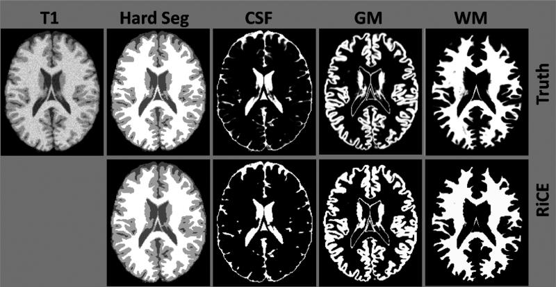
The phantom data comprises 15 phantoms, with 5 different noise levels (0-9%) and 3 different inhomogeneity levels (0, 20, 40%). Both the soft classification and the hard segmentation of the three tissues are shown in Fig. 3. The ground truth and the fuzzy memberships, from which the phantoms are generated, are also available and shown in the top row of Fig. 3. We use the true hard segmentation to find Dice coeffcients of the three tissue classes for each of the methods.
Figure 3.
Brainweb Phantom Validation: Comparison of RiCE (2nd row) with ground truth (1st row) on true hard segmentation and fuzzy membership functions of a Brainweb phantom with 3% noise.
Table 1 presents Dice coeffcients for each of the noise levels averaged over three inhomogeneity levels. RiCE is comparable to the other methods, ranking in the top two in 16 out of 20 cases. As the phantoms are corrupted by Rician noise (Cocosco et al., 1997), RiCE gives better CSF segmentation than the Gaussian based method (SPM) on low noise levels, with a slightly reduced performance on high noise levels (7-9%), where it becomes comparable to both FAST and SPM. FAST, Freesurfer, SPM and RiCE do not perform as well as FANTASM on low noise data. We believe the reason for this is the small standard deviation of the PDF of the tissue classes, for which the EM iterations become unstable and may not converge to the true minima.
Table 1.
Experiment on 15 Brainweb phantoms with 5 different noise levels, each at three different inhomogeneity levels (0, 20, 40%). The Dice coefficients between ground truth and hard segmentations of each tissue class, averaged over three inhomogeneity levels, are shown at each noise level. “Mean” is a weighted Dice, weighted by the volumes of each tissue class generated from the corresponding algorithm. The segmentation from Freesurfer is denoted as SURFER.
| Noise Level |
||||||
|---|---|---|---|---|---|---|
| 0% | 3% | 5% | 7% | 9% | ||
| CSF | FAST | 0.9312 | 0.9170 | 0.9295 | 0.9236 | 0.9255 |
| SURFER | 0.8560 | 0.8598 | 0.8561 | 0.8341 | 0.8014 | |
| FANTASM | 0.9520 | 0.9456 | 0.9350 | 0.9176 | 0.8978 | |
| SPM | 0.9700 | 0.9547 | 0.9400 | 0.9266 | 0.9010 | |
| RiCE | 0.9561 | 0.9500 | 0.9411 | 0.9301 | 0.9266 | |
| GM | FAST | 0.8394 | 0.9347 | 0.9337 | 0.9251 | 0.9123 |
| SURFER | 0.8496 | 0.8969 | 0.8611 | 0.8064 | 0.7474 | |
| FANTASM | 0.9682 | 0.9582 | 0.9429 | 0.9179 | 0.8881 | |
| SPM | 0.8997 | 0.9590 | 0.9426 | 0.9248 | 0.8952 | |
| RiCE | 0.9465 | 0.9580 | 0.9444 | 0.9250 | 0.9100 | |
| WM | FAST | 0.7448 | 0.9628 | 0.9545 | 0.9416 | 0.9292 |
| SURFER | 0.8691 | 0.9602 | 0.9230 | 0.8733 | 0.8231 | |
| FANTASM | 0.9734 | 0.9647 | 0.9511 | 0.9304 | 0.9020 | |
| SPM | 0.8483 | 0.9541 | 0.9575 | 0.9355 | 0.9014 | |
| RiCE | 0.9718 | 0.9710 | 0.9654 | 0.9332 | 0.9322 | |
| Mean | FAST | 0.8318 | 0.9405 | 0.9401 | 0.9324 | 0.9209 |
| SURFER | 0.8569 | 0.9105 | 0.8819 | 0.8362 | 0.7861 | |
| FANTASM | 0.9670 | 0.9581 | 0.9443 | 0.9231 | 0.8949 | |
| SPM | 0.8977 | 0.9518 | 0.9471 | 0.9308 | 0.9033 | |
| RiCE | 0.9609 | 0.9589 | 0.9548 | 0.9262 | 0.9294 | |
4.2. IBSR Validation
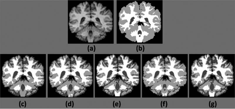
The next validation experiment was conducted on 18 normal healthy subjects from the Internet Brain Segmentation Repository (IBSR) (Center for Morphometric Analysis (CMA), 1995). The MR brain data sets and their manual segmentations were provided by the Center for Morphometric Analysis at Massachusetts General Hospital. The T1-w coronal data is acquired on a 1.5T scanner. The manual whole head segmentations are used as a ground truth. Fig. 4 shows a slice of an image, with the manual and automatic segmentations from the five methods. As the manual segmentation does not include cortical CSF as a class, we combine CSF and GM as one class to compute Dice between the manual segmentation and the automatic segmentations. Table 2 shows the Dice coe -cients of hard segmentation from each algorithm.
Figure 4.
Comparison of hard segmentations of normal IBSR subject, (a) A T1 SPGR acquisition, (b) manual segmentation of WM and GM, (c) segmentation by FAST, (d) segmentation by FANTASM, (e) FCM based segmentation by Freesurfer, (f) segmentation by SPM, (g) segmentation by RiCE.
Table 2.
Experiment with 18 normal IBSR subjects: Mean and standard deviations of Dice coefficients of GM, WM, and a volume weighted average (WA) between manual segmentations and hard segmentations obtained by FAST, FANTASM (FN), Freesurfer FCM based segmentation (SURF), SPM and RiCE are shown.
| FAST | FN | SURF | SPM | RiCE | ||
|---|---|---|---|---|---|---|
| GM | Mean | 0.9271 | 0.9186 | 0.9340 | 0.9131 | 0.9366 |
| Std | 0.0109 | 0.0099 | 0.0076 | 0.0217 | 0.0077 | |
| WM | Mean | 0.8685 | 0.8685 | 0.8660 | 0.8558 | 0.8652 |
| Std | 0.0105 | 0.184 | 0.0151 | 0.0283 | 0.0169 | |
| WA | Mean | 0.9071 | 0.9100 | 0.9128 | 0.9030 | 0.9127 |
| Std | 0.0106 | 0.0132 | 0.0095 | 0.0251 | 0.0121 | |
RiCE holds a higher score than FAST, SPM and FANTASM for GM segmentation, yielding a statistically significant improvement in these two cases (p-values of 0.012, 0.00002, 0.34 and 0.0004 for a pairwise t-test with FAST, FANTASM, Freesurfer and SPM, respectively). For the WM segmentation, the performance of RiCE is not significantly different from the others. This experiment thus indicates that making the more rigorous Rician assumption does not deteriorate the performance of WM and GM segmentation and the segmentations from RiCE are comparable to those from the current available methods on WM and GM.
In the following sections, we will show the e cacy of using the Rician model over a comparable Gaussian one, by showing the improvement in segmentation consistency, both in terms of tissue classes as well as cortical surfaces.
5. Comparison with a Gaussian model
5.1. Segmentation consistency
We carry out a consistency performance experiment on a set of 3T data from the Baltimore Longitudinal Study of Aging (BLSA) (Shock et al., 1984; Resnick et al., 2003), comprised of T1w axial MPRAGE and SPGR acquisitions (256 × 256 × 124 volumes having the resolution of 0.9375 × 0.9375 × 1.5 mm) of 14 normal subjects, ages in the range of 69 – 92. The SPGR acquisitions are registered to their corresponding MPRAGE acquisition using a rigid registration (Jenkinson and Smith, 2001) and stripped using a hybrid registration based skull-stripping algorithm (Carass et al., 2007, 2011). Then each of the images is bias-corrected using N3.
Ideally, we expect to be able to generate identical segmentations of each subject from the different acquisitions. Then we modify Eqn. 5 keeping the smoothness fMRF,while changing the Rician PDF fR(y|v, σ) from Eqn. 1 to a Gaussian one , thereby modifying the Eqns. 10–14 accordingly.
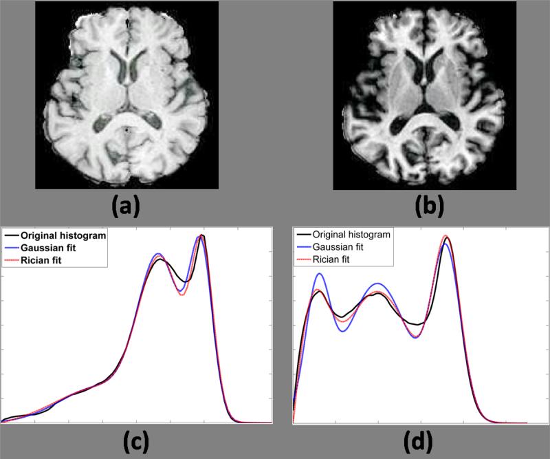
Average Dice coeffcients between the hard segmentations obtained from SPGR and MPRAGE acquisitions of the same subject are reported in Table 3. The consistency improves significantly on CSF segmentation, which is expected because the Rician distribution models the CSF intensity regime better than a Gaussian one, as seen by the fitting of the histograms of the SPGR and MPRAGE images, shown in Fig. 5(c)-(d). The KL distance between the actual histogram and the Rician and Gaussian fitting is 0.0129 and 0.0342, respectively, for MPRAGE, and 0.0876 and 0.1012 for SPGR. Thus, better fitting of the histograms provide more accurate delineation between the tissue classes. There is a large variability in the GM segmentation for both the Rician and the Gaussian models, which can be explained by the variability of the intensities of the sub-cortical structures, which is not explicitly modeled in this scenario.
Table 3.
Dice comparison of Rician and Gaussian mixture models on BLSA data: Segmentation consistency of the Rician model is compared with a similar method having a Gaussian model, keeping the smoothness assumption the same. Dice coefficients between the segmentations of bias-corrected (Sled et al., 1998) SPGR and MPRAGE acquisitions of the same subject are shown for CSF, GM, WM and a weighted average (WA), weighted by the individual volumes of the tissues. Mean and standard deviations (Std) are calculated based on 14 normal subjects. The p-value for a null hypothesis, that the CSF Dice coefficient for Rician model is smaller than that of the Gaussian model, is 0.0001. The p-values for a similar hypothesis on the GM, WM and WA Dice coefficients are 0.022, 0.001, 0.011, respectively.
| CSF |
GM |
WM |
WA |
|||||
|---|---|---|---|---|---|---|---|---|
| Mean | Std | Mean | Std | Mean | Std | Mean | Std | |
| Gauss | 0.6872 | 0.0429 | 0.6700 | 0.0544 | 0.8205 | 0.0367 | 0.7376 | 0.0423 |
| Rice | 0.7589 | 0.0386 | 0.7289 | 0.0384 | 0.8535 | 0.0200 | 0.7924 | 0.0249 |
Figure 5.
Rician and Gaussian fitting of histograms : (a) SPGR acquisition, (b) MPRAGE acquisition, (c) the best fit of the SPGR histogram and (d) the best fit of the MPRAGE histogram by a Gaussian and a Rician mixture model are also shown. The KL distances between the histogram and the Rician and Gaussian fitting are 0.0129 and 0.0342 for MPRAGE, and 0.0876 and 0.1012 for SPGR, respectively.
5.2. Cortical surface consistency
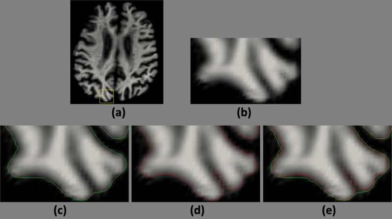
Cortical thickness is an important measure for the neuroscience community (Querbes et al., 2009; Evans et al., 2005). As a consequence, robust and accurate delineation of cortical surfaces are of importance. We study the Rician model on the consistent delineation of the cortical surfaces. We use a Cortical Reconstruction Using Implicit Surface Evolution (CRUISE) (Han et al., 2004) to generate inner and outer surfaces from the soft classification. As the Rician model is most effective in modeling the CSF intensities (see Fig. 5), we expect the CSF delineation to be more accurate, which is shown in Fig. 6. The CSF distribution in the image histogram is poorly fitted by a Gaussian in Fig. 5(d), which results in a under-estimation of the CSF-GM boundary, shown in Fig. 6(c), while a Rician model fits the histogram better and results in a more accurate estimate of the outer surface (Fig. 6(d)).
Figure 6.
Outer surface delineation, comparison between the Rician model and a Gaussian one: (a) An MPRAGE image, (b) its zoomed in view, (c) outer surface generated by CRUISE (Han et al., 2004) using the soft classification obtained using a Gaussian model (Sec. 5), (d) outer surface generated by the Rician model, (e) overlaid version of the two outer surfaces.
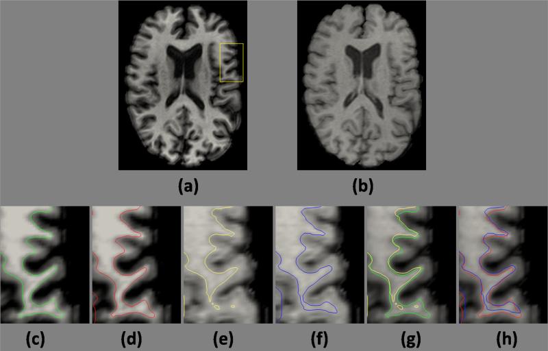
To show the improved consistency, we compare the cortical surfaces generated from the SPGR and MPRAGE acquisitions of the same subject. This is also shown in Fig. 7, where the inner surfaces generated using the Rician model are closer in these two acquisitions. The Gaussian model does not lead to accurate estimation of the inner surface on the SPGR image due to the poor GM-WM contrast and the heavy partial volume effect (Fig. 7(e)), while a Rician model is better in this scenario (Fig. 7(f)). Quantitative distance between these surfaces are reported in Table 4. The surface distance is the mean of the distances between one surface and the other, while the distance from a point on the surface is the shortest distance to the other surface.. The results are averaged on a pool of 14 normal subjects. A significantly large improvement in average inner surface difference is observed with the Rician model.
Figure 7.
Comparison of the consistency in inner cortical surface between the Rician model and a Gaussian one: (a) MPRAGE and (b) SPGR acquisition of the same subject, inner surfaces of the MPRAGE image obtained using (c) Gaussian and (d) Rician model, inner surfaces of the SPGR image obtained using (e) Gaussian and (f) Rician model, overlaid (on the MPRAGE) version of the surfaces obtained using (g) Gaussian and (h) Rician model.
Table 4.
Surface Differences between Gaussian and Rician models : Cortical surfaces are generated by CRUISE (Han et al., 2004) from soft classifications generated by RiCE and a comparable Gaussian model on 14 BLSA subjects. The experiment is described in Sec. 5. The mean difference (mm) between inner (and outer) surfaces, generated from SPGR and MPRAGE images, are given. Using a null hypothesis that the surface differences arising from RiCE are smaller than that of the corresponding Gaussian model, the p-values obtained from a t-test are 0.00001 and 0.022 for inner and outer surfaces, respectively.
| Inner Surface |
Outer Surface |
|||
|---|---|---|---|---|
| Mean | Std | Mean | Std | |
| Gaussian | 1.2276 | 0.1807 | 0.7869 | 0.1497 |
| Rician | 0.7022 | 0.0987 | 0.6001 | 0.0901 |
6. Comparison with other methods
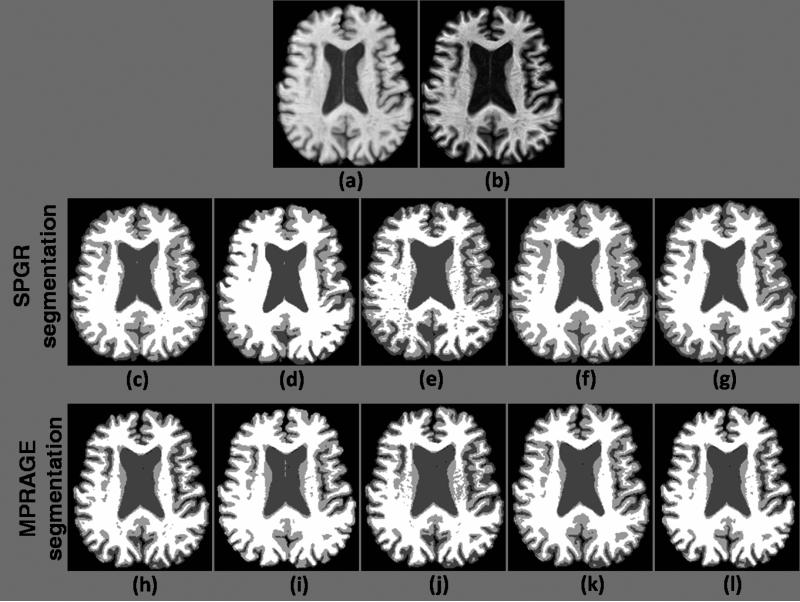
In this section, we compare the overall performance of our method with other methods. Fig. 8 shows the comparison of the hard segmentations using the 5 algorithms. The Dice coeffcients of the three classes and their volume weighted “average” Dice are shown in Table 5, which shows that both the CSF and GM segmentation are more similar in the case of RiCE. T-tests comparing the overlap of CSF and GM show a significant improvement in consistency over the other four methods. This experiment also shows that the Rician model does not do worse than a Gaussian model on WM segmentation. Thus the Rician model is significantly more consistent in a Gaussian model on low SNR regime.
Figure 8.
Segmentation Consistency : (a) SPGR acquisition, (b) MPRAGE acquisition, (c) FAST, (d) FANTASM, (e) Freesurfer (mri ms EM), (f) SPM (spm segment) and (g) RiCE hard segmentation of the SPGR image, (h) FAST, (i) FANTASM, (j) Freesurfer, (k) Freesurfer and (l) RiCE hard segmentation of the MPRAGE image.
Table 5.
Dice comparison of the consistency experiment: 14 subjects with both T1 SPGR and T1 MPRAGE acquisitions are processed with RiCE, FAST, FANTASM (FN), Freesurfer (SURF) and SPM segmentation. Dice coefficients between their hard segmentations are shown for CSF, GM, WM and a weighted average (WA), weighted by the individual volumes of the tissues, obtained from each of the algorithms. The p-values for a null hypothesis, that CSF Dice coefficient for RiCE is smaller than that of FAST/FANTASM/Freesurfer/SPM are 0.0016, 0.00001, 0.0002, 0.0046 respectively. The p-values for a similar hypothesis on the GM, WM and mean Dice coefficients (WA) are [0.0128, 0.009, 0.003, 0.25], [0.1258, 0.00001, 0.0002, 0.24] and [0.425, 0.0007, 0.0041, 0.07], respectively, where each quadruplet denotes the comparison of RiCE with FAST/FANTASM/Freesurfer/SPM.
| FAST | FN | SURF | SPM | RiCE | ||
|---|---|---|---|---|---|---|
| CSF | Mean | 0.6758 | 0.6317 | 0.6829 | 0.7207 | 0.7589 |
| Std | 0.0431 | 0.0504 | 0.0401 | 0.0264 | 0.0386 | |
| GM | Mean | 0.6889 | 0.6697 | 0.6381 | 0.7201 | 0.7289 |
| Std | 0.0621 | 0.0549 | 0.0690 | 0.0280 | 0.0384 | |
| WM | Mean | 0.8288 | 0.7960 | 0.8141 | 0.8589 | 0.8535 |
| Std | 0.0329 | 0.0274 | 0.0352 | 0.0195 | 0.0200 | |
| WA | Mean | 0.7392 | 0.7151 | 0.7309 | 0.7785 | 0.7924 |
| Std | 0.0407 | 0.0358 | 0.0376 | 0.0220 | 0.0249 | |
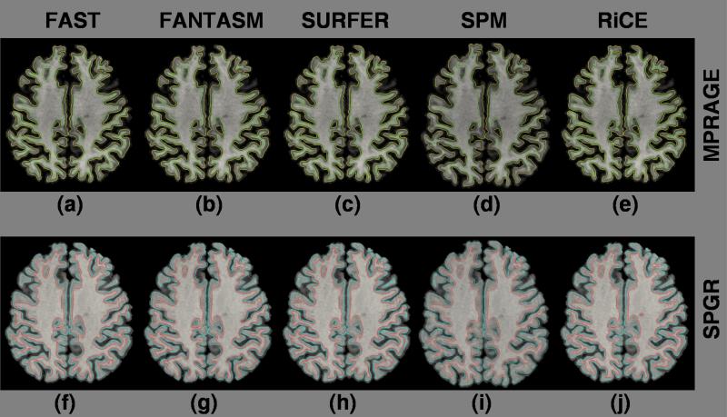
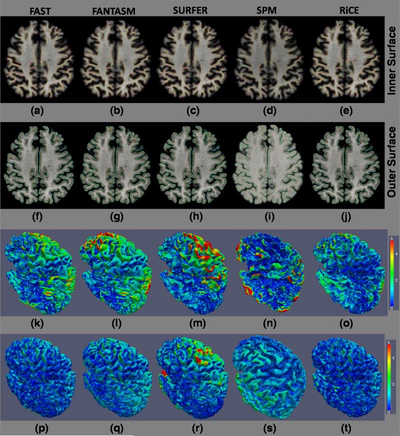
Fig. 9 shows a visual comparison of the surfaces using the soft classification from FAST, FANTASM, Freesurfer, SPM and RiCE. The difference (in mm) between the inner (and outer) surfaces generated from SPGR and MPRAGE acquisitions are given in Table 6 and a visual comparison of the difference is shown in Fig. 10. The statistical tests, reported in Table 6, also confirm that RiCE produces more consistent cortical surface delineation.
Figure 9.
Cortical surfaces from two different acquisitions : Inner (green) and outer (yellow) surfaces of the MPRAGE processed by (a) FAST, (b) FANTASM, (c) Freesurfer (mri ms EM), (d) SPM (spm segment) and (e) RiCE. Inner (red) and outer (blue) surfaces of SPGR processed by (f) FAST, (g) FANTASM, (h) Freesurfer, (i) SPM and (j) RiCE.
Table 6.
Surface differences of the consistency experiment : Cortical surfaces are generated by CRUISE (Han et al., 2004) from soft classifications generated by FAST, FANTASM (FN), Freesurfer (SURF), SPM and RiCE. The mean surface difference in mm, averaged over 14 normal subjects, between surfaces (shown in Fig. 10) generated from SPGR and MPRAGE images are reported. The experiment is described in Sec. 6. Using a null hypothesis that the inner surface differences arising from FAST/FN/SURF/SPM are smaller than that of RiCE, the p-values obtained from a t-test are 0.0004, 0.000006, 0.0003 and 0.0421, respectively. A similar hypothesis on the outer surfaces give the following p-values 0.0032, 0.000001 and 0.000001 and 0.00005 for FAST/FN/SURF/SPM, respectively.
| Inner Surface |
Outer Surface |
|||
|---|---|---|---|---|
| Mean | Std | Mean | Std | |
| FAST | 0.8852 | 0.1996 | 0.7607 | 0.1376 |
| FN | 1.2375 | 0.1997 | 0.9234 | 0.0891 |
| SURF | 1.0356 | 0.1551 | 0.9446 | 0.2042 |
| SPM | 0.7829 | 0.0949 | 0.8213 | 0.0917 |
| RiCE | 0.7106 | 0.1017 | 0.6114 | 0.1001 |
Figure 10.
Surface difference between The cortical surfaces generated from the SPGR and MPRAGE are shown on the MPRAGE image. Inner surface of the MPRAGE (green) and SPGR (red) processed by (a) FAST, (b) FANTASM, (c) Freesurfer (mri_ms_EM), (d) SPM (spm_segment) and (e) RiCE are shown on the MPRAGE. Outer surface of the MPRAGE (yellow) and SPGR (blue) processed by (f) FAST, (g) FANTASM, (h) Freesurfer, (i) SPM and (j) RiCE are shown on the SPGR image. A color map of the absolute difference between the inner surfaces of SPGR and MPRAGEs, obtained from the five algorithms, are shown in (k)-(o). Similarly, the color map of the difference between the outer surfaces of SPGR and MPRAGEs are shown in (p)-(t). RiCE gives overall smaller surface difference (see Table 6).
7. Summary and Conclusion
This paper proposes a Rician PDF based brain MR segmentation technique. We have concentrated on consistent segmentation of three primary tissues, cerebrospinal fluid, gray matter and white matter, from T1-weighted MR images acquired with two different pulse sequences, MPRAGE and SPGR. The underlying acquisition parameters, like repetition time, inversion time or flip angle, are usually different from one sequence to another, which gives rise to the variability of the tissue contrast. With exact knowledge of the acquisition parameters and the imaging sequences, consistent tissue segmentations can be obtained (Fischl et al., 2004), but for most studies, either the parameters are not available or the imaging sequences are diffcult to model accurately. Hence, most statistical segmentation algorithms rely on probabilistic modeling of the intensities only. It is diffcult to remove inconsistencies in the segmentations between images from different pulse sequences without the exact knowledge of the acquisition process, which is the primary source of the variability in the contrast.
Both SPGR and MPRAGE sequences are often used to obtain T1-w MR images. They are gradient-echo sequences, but have widely variable tissue contrast due to the difference in acquisition processes and the imaging parameters. Nevertheless, the MR image intensity at each voxel follows Rician distribution for both these pulse sequences, although most of the current statistical model based segmentation techniques assume an underlying Gaussian distribution. Specifically, it can be seen that CSF and GM, having low SNR in T1w images, are not modeled correctly by Gaussians (Fig. 1). As a result, the segmentations of T1w images with different pulse sequences become inconsistent. We have shown that introducing a Rician PDF produces more consistent segmentation between SPGR and MPRAGEs, both in terms of hard segmentation of tissues and delineation of cortical surfaces. The use of the Rician distribution to replace Gaussian distributions is shown to be promising, unfortunately the modeling of tissue classes in this manner is far from a satisfactory solution. Modeling tissue classes in this mono-model manner ignores the true complexity of tissue structures and the local variation that is possible within a tissue. This topic, in light of this advancement in the correct tissue model, is a rich area for future work.
Our algorithm is fully automatic and no training data is required. We correct the image inhomogeneities by a non-parametric model and use Markov random field to introduce segmentation consistency. We have validated the algorithm on the Brainweb phantom and IBSR 20 normal subjects. The improvement in segmentation consistency is demonstrated on 14 BLSA subjects having both SPGR and MPRAGE scans. The algorithm takes approximately 10 minutes on a 3GHz Intel processor on a Linux workstation. Future work will focus on incorporating a priori information via statistical atlases.
 Noise in magnetic resonance images should be modeled as Rician distribution.
 Rician distribution fits the MR image histogram better than a Gaussian one.
 Cortical surfaces from the brain MR images can be better delineated using Rician models in a segmentation algorithm compared to a Gaussian one.
 Segmentation between same brain MR images acquired under different pulse sequences are more consistent using Rician modeling.
Acknowledgment
This research was supported in part by the Intramural Research Program of the NIH, National Institute on Aging. We are grateful to all the participants of the Baltimore Longitudinal Study on Aging (BLSA), as well as the neuroimaging sta for their dedication to these studies. This work was also supported by the NIH/NINDS under grant 5R01NS037747.
Appendix
A brief derivation of Eqn. 11 to Eqn. 14 are given in this appendix.
To do the E-step, we find the as
where fMRF(zjk|zNj, Θ(m)) is given by Eqn. 8. Using mean-field approximation (Zhang, 1992) to replace zjk by the current estimate of its expectation , we obtain Eqn. 11.
The M-step provides the estimation of Θ from Eqn. 9.
Q(Θ(m+1)|Θ(m)) becomes,
We note that the 1st term of is explicitly independent of and and the 2nd term is explicitly independent of . So is maximized w.r.t. , by setting the partial derivative of the 2nd term w.r.t. to zero,
Simplifying this equation and also using the fact that a coordinate descent equation for is obtained in Eqn. 12.
Similarly, Eqn. 13 is obtained by setting the partial derivative of the 2nd term w.r.t. to zero.
As the 2nd term of is explicitly independent of , we equate the partial derivative of w.r.t to zero,
to get update equation Eqn. 14.
Footnotes
Publisher's Disclaimer: This is a PDF file of an unedited manuscript that has been accepted for publication. As a service to our customers we are providing this early version of the manuscript. The manuscript will undergo copyediting, typesetting, and review of the resulting proof before it is published in its final citable form. Please note that during the production process errors may be discovered which could affect the content, and all legal disclaimers that apply to the journal pertain.
References
- Ashburner J, Friston KJ. Voxel-Based Morphometry – The Methods. NeuroImage. 2000;11(6):805–821. doi: 10.1006/nimg.2000.0582. [DOI] [PubMed] [Google Scholar]
- Ashburner J, Friston KJ. Unified segmentation. NeuroImage. 2005;26(3):839–851. doi: 10.1016/j.neuroimage.2005.02.018. [DOI] [PubMed] [Google Scholar]
- Awate SP, Tasdizen T, Foster N, Whitaker RT. Adaptive Markov modeling for mutual-information-based, unsupervised MRI brain-tissue classification. Medical Image Analysis. 2006;10(5):726–739. doi: 10.1016/j.media.2006.07.002. [DOI] [PubMed] [Google Scholar]
- Bazin PL, Pham DL. Topology-preserving tissue classification of magnetic resonance brain images. IEEE Trans. on Medical Imaging. 2007;26(4):487–496. doi: 10.1109/TMI.2007.893283. [DOI] [PubMed] [Google Scholar]
- Bernstein MA, Thomasson DM, Perman WH. Improved detectability in low signal-to-noise ratio magnetic resonance images by means of a phase-corrected real reconstruction. Med. Physics. 1989;16(5):813–817. doi: 10.1118/1.596304. [DOI] [PubMed] [Google Scholar]
- Besag J. Spatial interaction and the statistical analysis of lattice systems. Journal of the Royal Stat. Soc. 1974;36(2):192–236. [Google Scholar]
- Bezdek JC. A Convergence Theorem for the Fuzzy ISODATA Clustering Algorithms. IEEE Trans. on Pattern Anal. Machine Intell. 1980 January;2(1):1–8. doi: 10.1109/tpami.1980.4766964. [DOI] [PubMed] [Google Scholar]
- Bezdek JC, Hall LO, Clarke LP. Review of MR image segmentation techniques using pattern recognition. Medical Physics. 1993;20:1033–1048. doi: 10.1118/1.597000. [DOI] [PubMed] [Google Scholar]
- Carass A, Cuzzocre J, Wheeler MB, Bazin PL, Resnick SM, Prince JL. Simple paradigm for extra-cerebral tissue removal: Algorithm and analysis. NeuroImage. 2011;56(4):1982–1992. doi: 10.1016/j.neuroimage.2011.03.045. [DOI] [PMC free article] [PubMed] [Google Scholar]
- Carass A, Wheeler MB, Cuzzocreo J, Bazin PL, Bassett SS, Prince JL. A Joint Registration and Segmentation Approach to Skull Stripping. IEEE Intl. Symp. on Biomed. Imag. (ISBI) 2007:656–659. [Google Scholar]
- Cavalcanti N, de Carvalho FAT. An Adaptive Fuzzy C-Means Algorithm with the L2 Norm. Australian Conf. in. Artificial Intell. 2005:1138–1141. [Google Scholar]
- Center for Morphometric Analysis (CMA) Internet Brain Segmentation Repository. 1995 URL http://www.cma.mgh.harvard.edu/ibsr/
- Chang H, Fitzpatrick JM. A technique for accurate magnetic resonance imaging in the presence of field inhomogeneities. IEEE Trans. on Med. Imag. 1992;11(3):319–329. doi: 10.1109/42.158935. [DOI] [PubMed] [Google Scholar]
- Chard DT, Parker GJ, Gri n CM, Thompson AJ, Miller DH. The reproducibility and sensitivity of brain tissue volume measurements derived from an SPM-based segmentation methodology. Journal of Magn. Reson. Imag. 2002;15(3):259–267. doi: 10.1002/jmri.10064. [DOI] [PubMed] [Google Scholar]
- Choi HS, Haynor DR, Kim Y. Partial volume tissue classification of multichannel magnetic resonance images- A Mixel model. IEEE Trans. on Med. Imag. 1991 September;10(3):395–407. doi: 10.1109/42.97590. [DOI] [PubMed] [Google Scholar]
- Clark KA, Woods RP, Rottenber DA, Toga AW, Mazziotta JC. Impact of acquisition protocols and processing streams on tissue segmentation of T1 weighted MR images. NeuroImage. 2006;29:185–202. doi: 10.1016/j.neuroimage.2005.07.035. [DOI] [PubMed] [Google Scholar]
- Cocosco CA, Kollokian V, Kwan RKS, Evans AC. BrainWeb: Online Interface to a 3D MRI Simulated Brain Database. NeuroImage. 1997;5(4):S425. URL http://www.bic.mni.mcgill.ca/brainweb/
- Dale AM, Fischl B, Sereno MI. Cortical Surface-Based Analysis I: Segmentation and Surface Reconstruction. NeuroImage. 1999;9(2):179–194. doi: 10.1006/nimg.1998.0395. [DOI] [PubMed] [Google Scholar]
- Dempster AP, Laird NM, Rubin DB. Maximum Likelihood from Incomplete Data via the EM Algorithm. Journal of Royal Stat. Soc. 1977;39:1–38. [Google Scholar]
- Diplaros A, Vlassis N, Gevers T. A spatially constrained generative model and an EM algorithm for image segmentation. IEEE Trans. Neural Netw. 2007;18(3):798–808. doi: 10.1109/TNN.2007.891190. [DOI] [PubMed] [Google Scholar]
- Evans AC, Lerch JP, Pruessner J, Zijdenbos AP, Teipe SJ, Hampe H. Cortical thickness in Alzheimers disease. Alzheimer's and Dementia. 2005;1(1):S7. [Google Scholar]
- Fischl B, Salat DH, van der Kouwe AJW, Makris N, Segonne F, Quinn BT, Dale AM. Sequence-independent segmentation of magnetic resonance images. NeuroImage. 2004;23:69–84. doi: 10.1016/j.neuroimage.2004.07.016. [DOI] [PubMed] [Google Scholar]
- Gudbjartsson H, Patz S. The Rician Distribution of Noisy MRI Data. Mag. Resonance in Med. 1995;34(6):910–914. doi: 10.1002/mrm.1910340618. [DOI] [PMC free article] [PubMed] [Google Scholar]
- Gustafson DE, Kessel W. Fuzzy clustering with a fuzzy covariance matrix. Proc. IEEE Conf. Decision Contr. 1979 January;:761–766. [Google Scholar]
- Han X, Fischl B. Atlas Renormalization for Improved Brain MR Image Segmentation Across Scanner Platforms. IEEE Trans. Med. Imag. 2007;26(4):479–486. doi: 10.1109/TMI.2007.893282. [DOI] [PubMed] [Google Scholar]
- Han X, Pham DL, Tosun D, Rettman RE, Xu C, Prince JL. CRUISE: Cortical Reconstruction Using Implicit Surface Evolution. NeuroImage. 2004;23(3):997–1012. doi: 10.1016/j.neuroimage.2004.06.043. [DOI] [PubMed] [Google Scholar]
- He R, Datta S, Tao G, Narayana PA. Information measures-based intensity standardization of MRI. Intl. Conf. Engg. in Med. and Biology Soc. 2008 August;:2233–2236. doi: 10.1109/IEMBS.2008.4649640. [DOI] [PubMed] [Google Scholar]
- Held K, Kops ER, Krause BJ, Wells WM, Kikinis R, Muller-Gartner H. Markov Random Field Segmentation of Brain MR Images. IEEE Trans. on Med. Imag. 1997;16(6):878–886. doi: 10.1109/42.650883. [DOI] [PubMed] [Google Scholar]
- Henkelman RM. Measurement of signal intensities in the presence of noise in MR images. Med. Phys. 1985;12(2):232–233. doi: 10.1118/1.595711. [DOI] [PubMed] [Google Scholar]
- Hong X, McClean S, Scotney B, Morrow P. Model-Based Segmentation of Multimodal Images. Comp. Anal. of Images and Patterns. 2007;4672:604–611. [Google Scholar]
- Jenkinson M, Smith S. A global optimisation method for robust affine registration of brain images. Medical Image Analysis. 2001;5(2):143–156. doi: 10.1016/s1361-8415(01)00036-6. [DOI] [PubMed] [Google Scholar]
- Kullback S, Leibler R. On Information and Sufficiency. Annals of Mathematical Statistics. 1951;22(1):79–86. [Google Scholar]
- Leemput KV, Bakkour A, Benner T, Wiggins G, Wald LL, Augustinack J, Dickerson BC, Golland P, Fischl B. Automated segmentation of hippocampal subfields from ultra-high resolution in vivo MRI. Hippocampus. 2009;19(6):549–557. doi: 10.1002/hipo.20615. [DOI] [PMC free article] [PubMed] [Google Scholar]
- Leemput KV, Maes F, Vandermeulen D, Suetens P. Automated Model-Based Tissue Classification of MR Images of the Brain. IEEE Trans. on Med. Imag. 1999;18(10):897–908. doi: 10.1109/42.811270. [DOI] [PubMed] [Google Scholar]
- Leemput KV, Maes F, Vandermeulen D, Suetens P. A Unifying Framework for Partial Volume Segmentation of Brain MR Images. IEEE Trans. on Med. Imag. 2003;22(1):105–119. doi: 10.1109/TMI.2002.806587. [DOI] [PubMed] [Google Scholar]
- Li SZ. Markov Random Field Modeling in Computer Vision. IEEE Conf. on Comp. Vision Patt. Recog. 1995:264–276. [Google Scholar]
- Li SZ. Markov random field modeling in image analysis. Springer-Verlag New York, Inc.; Secaucus, NJ, USA: 2001. [Google Scholar]
- Mangin JF. Entropy minimization for automatic correction of intensity nonuniformity. IEEE Workshop on Math. Methods in Biomed. Image Anal. 2000:162–169. [Google Scholar]
- Manjon JV, Lull JJ, Carbonell-Caballero J, Garcia-Marti G, Marti-Bonmati L, Robles M. A nonparametric MRI inhomogeneity correction method. Med. Imag. Anal. 2007;11(4):336–345. doi: 10.1016/j.media.2007.03.001. [DOI] [PubMed] [Google Scholar]
- Mueller SG, Weiner MW, Thal LJ, Petersen RC, Jack C, Jagust W, Trojanowski JQ, Toga AW, Beckett L. The Alzheimers Disease Neuroimaging Initiative. Neuroimaging Clin. N. Am. 2005;15(4):869–877. doi: 10.1016/j.nic.2005.09.008. [DOI] [PMC free article] [PubMed] [Google Scholar]
- Neal RM, Hinton GE. A view of the EM algorithm that justifies incremental, sparse, and other variants. MIT Press. 1999:355–368. [Google Scholar]
- Nikou C, Galatsanos N, Likas AC. A Class-Adaptive Spatially Variant Mixture Model for Image Segmentation. IEEE Trans. on Imag. Proc. 2007;16(4):1121–1130. doi: 10.1109/tip.2007.891771. [DOI] [PubMed] [Google Scholar]
- Noe A, Gee JC. Efficient Partial Volume Tissue Classification in MRI Scans. Med. Image Comp. and Comp.-Asst. Intervention (MICCAI) 2002;2488:698–705. [Google Scholar]
- Nyul LG, Udupa JK. On Standardizing the MR Image Intensity Scale. Mag. Res. in Medicine. 1999;42(6):10721081. doi: 10.1002/(sici)1522-2594(199912)42:6<1072::aid-mrm11>3.0.co;2-m. [DOI] [PubMed] [Google Scholar]
- Pham DL. Spatial models for fuzzy clustering. Comp. Vision & Image Understand. 2001;84(2):285–297. [Google Scholar]
- Pham DL, Prince JL. Adaptive Fuzzy Segmentation of Magnetic Resonance Images. IEEE Trans. on Med. Imag. 1999;18(9):737–752. doi: 10.1109/42.802752. [DOI] [PubMed] [Google Scholar]
- Potts RB. Some generalized order-disorder transformations. Proc. of the Cambridge Philosophical Soc. 1952;48:106–109. [Google Scholar]
- Prastawa M, Gilmore J, Lin W, Gerig G. Automatic segmentation of neonatal brain MRI. Proc. Int. Conf. Med. Image Comput. Comput. Assisted Intervention (MICCAI) 2004:10–17. [Google Scholar]
- Prince JL, Tan Q, Pham DL. Optimization of MR Pulse Sequences for Bayesian Image Segmentation. Medical Physics. 1995 October;22(10):1651–1656. doi: 10.1118/1.597425. [DOI] [PubMed] [Google Scholar]
- Querbes O, Aubry F, Pariente J, Lotterie J, Demonet J, Duret V, Puel M, Berry I, Fort J, Celsis P, Initiative TADN. Early diagnosis of Alzheimer's disease using cortical thickness: impact of cognitive reserve. Brain. 2009;132(8):2036–2047. doi: 10.1093/brain/awp105. [DOI] [PMC free article] [PubMed] [Google Scholar]
- Raz N, Rodrigue KM, Acker J. Hypertension and the brain: Vulnerability of the prefrontal regions and executive functions. Behavioral Neuroscience. 2003;117(6):1169–1180. doi: 10.1037/0735-7044.117.6.1169. [DOI] [PubMed] [Google Scholar]
- Resnick SM, Pham DL, Kraut MA, Zonderman AB, Davatzikos C. Longitudinal magnetic resonance imaging studies of older adults: A shrinking brain. Journal of Neuroscience. 2003;23(8):3295–3301. doi: 10.1523/JNEUROSCI.23-08-03295.2003. [DOI] [PMC free article] [PubMed] [Google Scholar]
- Rice SO. Mathematical Analysis of Random Noise. In: Wax N, editor. Selected Papers on Noise and Stochastic Processes. Dover Pubns; Jun, 1954. [Google Scholar]
- Rousseau F. Brain Hallucination. European Conf. on Comp. Vision. 2008:497–508. [Google Scholar]
- Roy S, Agarwal H, Carass A, Bai Y, Pham DL, Prince JL. Fuzzy c-means with variable compactness. Intl. Symp. on Biomed. Imag. 2008 June;:452–455. doi: 10.1109/ISBI.2008.4541030. [DOI] [PMC free article] [PubMed] [Google Scholar]
- Sanjay-Gopal S, Herbert TJ. Bayesian Pixel Classification Using Spatially Variant Finite Mixtures and the Generalized EM Algorithm. IEEE Trans. on Imag. Proc. 1998;7(7):1014–1028. doi: 10.1109/83.701161. [DOI] [PubMed] [Google Scholar]
- Scherrer B, Forbes F, Garbay C, Dojat M. Fully Bayesian Joint Model for MR Brain Scan Tissue and Structure Segmentation. Med. Image Comp. and Comp. Asst. Intervention (MIC-CAI) 2008;5242:1066–1074. doi: 10.1007/978-3-540-85990-1_128. [DOI] [PubMed] [Google Scholar]
- Shock NW, Gruelich R, Andres RA, Arenberg D, Costa PT, Lakatta EG, Tobin JD. Tech. rep. NIA; 1984. Normal Human Aging: The Baltimore Longitudinal Study of Aging. [Google Scholar]
- Sijbers J, Dekker AJ, Scheunders P, Dyck DV. Maximum-Likelihood Estimation of Rician Distribution Parameters. IEEE Trans. on Med. Imag. 1998;17(3):357–361. doi: 10.1109/42.712125. [DOI] [PubMed] [Google Scholar]
- Siyal MY, Yu L. An intelligent modified fuzzy c-means based algorithm for bias estimation and segmentation of brain MRI. Patt. Recog. Letters. 2005;26(13):2052–2062. [Google Scholar]
- Sled JG, Zijdenbos AP, Evans AC. A non-parametric method for automatic correction of intensity non-uniformity in MRI data. IEEE Trans. on Med. Imag. 1998;17(17):87–97. doi: 10.1109/42.668698. [DOI] [PubMed] [Google Scholar]
- Souza A, Senn R. Model-based super-resolution for MRI. Intl. Conf. on Engg. in Med. and Biology Soc. 2008 August;:430–434. doi: 10.1109/IEMBS.2008.4649182. [DOI] [PubMed] [Google Scholar]
- Styner M, Brechbuhler C, Szekely G, Gerig G. Parametric Estimate of Intensity Inhomogeneities applied to MRI. IEEE Trans. on Med. Imag. 2000;19(3):153–165. doi: 10.1109/42.845174. [DOI] [PubMed] [Google Scholar]
- Tu Z, Zheng S, Yuille AL, Reiss AL, Dutton RA, Lee AD, Galaburda AM, Dinov I, Thompson PM, Toga AW. Automated Extraction of the Cortical Sulci Based on a Supervised Learning Approach. IEEE Trans. on Med. Imag. 2007 April;26(4):541–552. doi: 10.1109/TMI.2007.892506. [DOI] [PubMed] [Google Scholar]
- Vovk U, Pernu F, Likar B. Multi-feature Intensity Inhomogeneity Correction in MR Images. Med. Image Comp. and Comp.-Asst. Intervention (MICCAI) 2004;3216:283–190. [Google Scholar]
- Wikipedia 2011 URL http://en.wikipedia.org/wiki/Rician distribution.
- Wolz R, Heckemann RA, Aljabar P, Hajnal JV, Hammers A, Ltjnen J, Rueckert D, The Alzheimer's Disease Neuroimaging Initiative Measurement of hippocampal atrophy using 4D graph-cut segmentation: Application to ADNI. NeuroImage. 2010;52(1):109–118. doi: 10.1016/j.neuroimage.2010.04.006. [DOI] [PubMed] [Google Scholar]
- Woolrich MW, Jbabdi S, Patenaude B, Chappell M, Makni S, Behrens T, Beckmann C, Jenkinson M, Smith SM. Bayesian analysis of neuroimaging data in FSL. NeuroImage. 2009;45:S173–186. doi: 10.1016/j.neuroimage.2008.10.055. [DOI] [PubMed] [Google Scholar]
- Wua J, Chung ACS. A novel framework for segmentation of deep brain structures based on Markov dependence tree. NeuroImage. 2009;46(4):1027–1036. doi: 10.1016/j.neuroimage.2009.03.010. [DOI] [PubMed] [Google Scholar]
- Yu J, Cheng Q, Huang H. Analysis of the weighting exponent in the FCM. IEEE Trans. Syst. Man and Cybernatics. 2004 February;34(1):634–639. doi: 10.1109/tsmcb.2003.810951. [DOI] [PubMed] [Google Scholar]
- Zhang J. The mean field theory in EM procedures for Markov random fields. IEEE Trans. on Signal Proc. 1992;40(10):2570–2583. doi: 10.1109/83.210863. [DOI] [PubMed] [Google Scholar]
- Zhang Y, Brady M, Smith S. Segmentation of Brain MR Images Through a Hidden Markov Random Field Model and the Expectation-Maximization Algorithm. IEEE Trans. on Med. Imag. 2001;20(1):45–57. doi: 10.1109/42.906424. [DOI] [PubMed] [Google Scholar]


