Modelling and disentangling physiological mechanisms: linear and nonlinear identification techniques for analysis of cardiovascular regulation

Abstract

Cardiovascular (CV) regulation is the result of a number of very complex control interactions. As computational power increases and new methods for collecting experimental data emerge, the potential for exploring these interactions through modelling increases as does the potential for clinical application of such models. Understanding these interactions requires the application of a diverse set of modelling techniques. Several recent mathematical modelling techniques will be described in this review paper. Starting from Granger's causality, the problem of closed-loop identification is recalled. The main aspects of linear identification and of grey-box modelling tailored to CV regulation analysis are summarized as well as basic concepts and trends for nonlinear extensions. Sensitivity analysis is presented and discussed as a potent tool for model validation and refinement. The integration of methods and models is fostered for a further physiological comprehension and for the development of more potent and robust diagnostic tools.

1. Introduction

Cardiovascular (CV) control depends on a number of complex interacting feedback mechanisms that depend on information from several sensor sites. The information on the state of the system is processed in the central autonomic control centre in the brain. This control centre generates autonomic nervous system outflow that is conveyed to the CV system by parasympathetic and sympathetic pathways which, in most instances, elicit opposite actions to maintain homeostasis. Transport via the blood stream is subject to both localized control through heart rate and contractility as well as highly distributed resistive and capacitive modulation in arterial and venous compartments. The latter, in turn, are governed by both the local mechanisms and the neural outflow. Furthermore, the several afferent signals converge to the autonomic centres (signals from the cardiopulmonary, baroreceptive, chemoreceptive, muscular, etc.) and convey interferences from other processes (breathing, vasomotion, muscular activity and many others), while central and humoral processes exert continuous modulation (Hyndman et al. 1971; Akselrod et al. 1981; Koepchen 1984). These signal interactions are reflected in short-term cardiovascular variability (CVV).

The large number of dynamic responses and interactions involved in CV control renders it difficult to disentangle different regulation processes and creates the risk of not identifying significant parameters. The objective of this review paper is to summarize several recent mathematical modelling techniques in order to foster their application and future integration, and therefore advance the understanding and monitoring of CV control. More specifically, two basic approaches and trend lines are described in this work. The first one centring on CVV analysis (see §§2 and 3) attacks the problem by means of grey-box modelling fusing black-box identification with the internal modelling of subsystems (e.g. the arterial Windkessel) which can be better described a priori with few free parameters. The second approach (see §5) describes the role played by sensitivity analysis (SA) in model identification. Parametric SA offers several descriptors in order to restrict the parameter set, improve the model and the experimental design, and focus the most informative data subsets.

A third focus of this paper and core issue in CVV analysis is the well-recognized presence of nonlinear effects discussed in §4. Owing to these effects, besides linear parametric and non-parametric approaches, a wealth of studies applied nonlinear dynamic descriptors (entropies, correlation and fractal dimensions, Lyapunov coefficients, etc.) to CVV. As such, however, the contribution appeared rather phenomenological and poorly integrated with a parametric causal interaction analysis, which was conversely restricted to linear features of small variabilities. Recent nonlinear identification methods can provide further tools dealing with broader aspects of the addressed interactions and are summarized in the following (see §4). In this perspective, SA (see §5) gains further importance, since it moves the constraint of ‘small changes’ required for linearization from the data to errors.

2. Causality and closed-loop approaches

Short-term CVV represents both an invaluable scope on main vital processes and a challenge to modelling and analysis methods, owing to the many regulation processes that interact and interfere in a complex fashion. Given the introductory physiological portrait, the importance of feedback acting in a closed loop was soon recognized (Guyton & Harris 1951) together with the need of disentangling the contribution of the feedforward and feedback branches lumped inside the CVV data by means of suitable identification methods (Baselli et al. 1994; Xiao et al. 2005). In the following, a brief summary of the basic concepts of parametric closed-loop identification and causal analysis of multi-channel data will be provided.

The problem of disentangling feedforward and feedback pathways in a closed-loop setting can be solved with the direct approach considering the temporal relationships between the dynamics recorded at two opposite loop corners: typically a control and a controlled variable. A more fortunate condition, which is rare in physiological systems, implies the availability of external drives and permits an indirect approach. Overlooking the problem of re-entrant information owing to feedback exposes the analysis to severe biases; nonetheless, a correct hypothesis definition and testing process permits one to solve the problem by exploiting common open-loop identification algorithms. In addition, consistency, accuracy and lack of bias properties can be quantified. Briefly, estimates are consistent and unbiased if the model is correctly parametrized both in its deterministic (blocks within the loop connecting measured signals) and stochastic (blocks conveying unmeasured residuals) parts. The estimate of a pathway is accurate if the loop is randomly disturbed at the pathway input, and if disturbances are not stiffly compensated by the control action (Ljung 1999).

An analysis of the temporal relationships relies on Granger's causality and generally on a parametric description of dynamics. Parametric and non-parametric methods are largely equivalent if a joint process description of the signals in the loop is aimed at or if causal analysis is limited to detection (Geweke 1982). Conversely, causal relationships are more easily described by parametric methods, where parameters represent the gains of delayed effects.

Granger's (1963) definition of causality (G-causality) represents the main reference point in assessing temporal relationships between data series with broad generality from open- to closed-loop conditions and from linear to nonlinear relationships. If the prediction of a series {y} given the past of y itself (and of other explanatory variables, if any) is improved by considering the past of a further series {x}, then x G-causes y: x→y. First, generality stems from the consideration that x→y does not deny the possibility of y→x, in a closed loop. Second, only the information brought from the causing signal to the caused one is focused, with no a priori constraints on the predictor form or on the prediction evaluation. Linear and nonlinear predictors can be considered, and either a reduction of prediction error variance or information content can be assessed.

Interestingly, most linear and nonlinear parametric identification methods are based on prediction error optimization, hence strictly attain G-causality (Porta et al. 2009).

3. Linear closed-loop identification combined with physiological modelling

The transfer functions derived from linear closed-loop identification often reflect the aggregate behaviour of a number of distinct physiological mechanisms. The archetypical example is the transfer function relating beat-to-beat fluctuations in arterial blood pressure (ABP) to heart rate (HR), which characterizes the arterial HR baroreflex and encompasses the linear dynamic properties of the arterial baroreceptors, afferent nerve fibres, brainstem, efferent nerve fibres and sinoatrial node. By representing the (black box) transfer functions with (white box) physiological models, separate mechanisms may be disentangled and quantified. Two recent examples of this ‘grey-box’ modelling approach are reviewed at a high level below.

(a) Selective quantification of the cardiac sympathetic and parasympathetic nervous systems

Traditional HR power spectral indices are limited as measures of the autonomic nervous system. In particular, these indices neither offer an effective marker of the sympathetic nervous system (SNS), owing to its joint mediation with the parasympathetic nervous system (PNS) in the low frequency (0.04–0.15 Hz) regime, nor afford truly specific measures of the autonomic nervous system, owing to the input contributions to HR such as respiration and ABP.

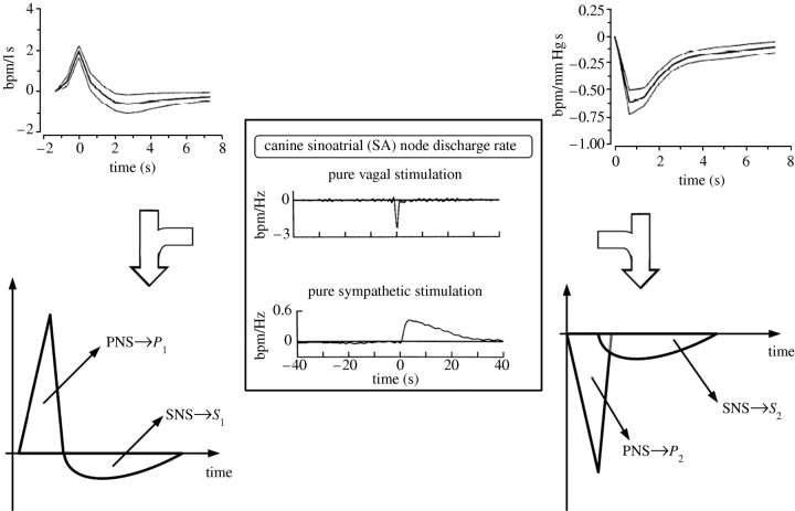
In two previous studies (Xiao et al. 2004; Chen & Mukkamala 2008), a new technique has been proposed to selectively quantify the SNS and PNS by multi-signal analysis of non-invasive cardiorespiratory measurements. The basic idea is to identify the transfer functions relating beat-to-beat fluctuations in ABP and instantaneous lung volume (ILV) to HR so as to remove the influence of the inputs on HR and then to model the identified transfer functions in the time domain rather than the frequency domain in order to disentangle the SNS from the PNS. More specifically, first, the impulse responses (time domain version of transfer functions) relating beat-to-beat fluctuations in ABP to HR (ABP→HR) and ILV to HR (ILV→HR) are estimated using linear closed-loop identification with two inputs. Then, the identified ABP→HR and ILV→HR impulse responses are each separated into an early and fast PNS component and a delayed and sluggish SNS component, and the two norms of these components are calculated so as to arrive at scalar indices of the PNS and SNS. This latter step is supported by the experimental data in figure 1, which suggest that the two identified impulse responses may each be modelled as a linear combination of experimentally derived impulse responses relating pure external vagal and sympathetic nervous stimulation to HR.

Figure 1.

Modelling the ILV→HR and ABP→HR impulse responses derived from linear closed-loop identification so as to disentangle the cardiac sympathetic nervous system (SNS) from the parasympathetic nervous system (PNS). ILV, instantaneous lung volume; HR, heart rate; ABP, arterial blood pressure. Adapted from Chen & Mukkamala (2008).

This technique was evaluated using selective pharmacological autonomic nervous blockade in 14 humans (Chen & Mukkamala 2008). The results showed that the indices obtained particularly from the ABP→HR impulse response were superior to traditional HR power spectral indices in terms of correctly predicting the known effects of atropine and/or propranolol on the SNS and PNS.

(b) Non-invasive quantification of the total peripheral resistance baroreflex

While HR variability is easy to measure, beat-to-beat fluctuations in total peripheral resistance (TPR) are not measurable and difficult to reliably estimate (Mukkamala et al. 2003). As a result, closed-loop identification has mainly been applied in the past to elucidate the feedback control of HR rather than TPR.

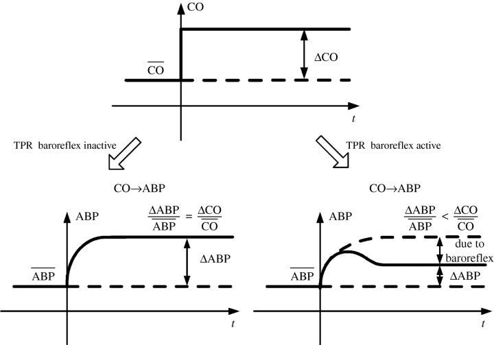
In a series of previous studies (Mukkamala et al. 2003, 2006; Chen et al. 2008), a novel technique has been progressively built to quantify the TPR baroreflex by analysis of only beat-to-beat measurements of ABP, cardiac output (CO) and stroke volume (SV). Significantly, these measurements may be obtained non-invasively in humans with, for example, finger-cuff photoplethysmography and Doppler ultrasound (Mukkamala et al. 2003). Rather than attempting to estimate the unobserved TPR fluctuations, the general idea is to account for these variations through the couplings between the measured fluctuations. For example, consider the ABP response to a step change in CO as shown in figure 2. If the TPR baroreflex were inactive, then, by Ohm's law, the steady-state fractional change in ABP would equal the fractional change in CO. However, if the TPR baroreflex were active, then the steady-state fractional change in ABP would be less than that of CO owing to the accompanying drop in TPR, with a smaller steady-state fractional ABP change indicating greater TPR baroreflex functioning. Following this intuitive example, first, the impulse responses (derivative of step responses) relating beat-to-beat fluctuations in CO to ABP (CO→ABP) and SV to ABP are estimated using linear closed-loop identification with two inputs. Then, the two identified impulse responses are each represented with physiological models so as to calculate the impulse response of the arterial TPR baroreflex, which relates beat-to-beat fluctuations in ABP to TPR, and the static gain value (area of the impulse response) of the cardiopulmonary TPR baroreflex, which relates beat-to-beat fluctuations in central venous transmural pressure to TPR. (Note that the residual variability in ABP not correlated with the fluctuations in CO and SV is assumed to be precisely due to non-baroreflex mechanisms such as local vascular control and central autonomic outflow.)

Figure 2.

Modelling the CO→ABP step response derived from linear closed-loop identification so as to quantify the total peripheral resistance (TPR) baroreflex. CO is cardiac output. Adapted from Mukkamala et al. (2006).

This technique was evaluated using chronic arterial baroreceptor denervation in seven conscious dogs instrumented with an aortic catheter and ultrasonic aortic flow probe (Mukkamala et al. 2006; Chen et al. 2008). Consistent with known physiology, the results showed that the arterial TPR baroreflex impulse response was virtually abolished following the chronic intervention, while the magnitude of the cardiopulmonary TPR baroreflex static gain value more than doubled perhaps due to a central compensatory mechanism.

4. Nonlinear closed-loop methods

Most, if not all, dynamics of physiological systems involve nonlinear control. For example, nonlinear feedback control mechanisms are important for maintaining homeostasis in the CV (Levy 1971; Saul et al. 1989; Chon et al. 1996) system. Closed-loop system identification analyses have mostly involved linear techniques, on the assumption that the contributions of the nonlinear components are small. This assumption has not been thoroughly tested primarily because nonlinear closed-loop methods that are computationally manageable and reasonably accurate have been lacking.

Recently, in recognition of the lack of nonlinear closed-loop parametric identification methods, Wang et al. (2007) introduced a nonlinear vector optimal parameter search (VOPS) algorithm, which is more accurate than the vector least squares (VLS). The VOPS owes its accuracy to the fact that it is able to extract only the significant parameters even in the condition of noise corruption and incorrect model selection (Lu et al. 2001; Zou et al. 2003; Wang et al. 2007). Furthermore, in this study, it was found that the total least squares (TLS) outperformed the least-squares-based methods especially when the system was corrupted with observation noise. Moreover, this study examined the effect of using an open-loop algorithm on a closed-loop system to quantify the error stemming from a wrong model assumption. In §4a, we briefly describe the four methods for closed-loop parametric identification: VLS; VOPS; COPS; and TLS.

(a) Methodologies

(i) Vector least squares applied to closed-loop nonlinear system identification

A two-channel closed-loop time-invariant nonlinear system with observation (η_x and η_y) and dynamic (ϵ_x and ϵ_y) noise can be described in the following matrix form:

(4.1)

and

(4.2)

where M is the order of the model, and ϵ_x and ϵ_y are the dynamic noise sources and η_x and η_y are the observation noise sources of the two channels. Both x′ and y′ denote the output signals owing to contamination by observation noise.

The VNAR model requires the use of vector Akaike's information criterion (AIC) or vector minimum description length (MDL) criterion to select the system's model order M (M=min(AIC(m)) in equation (4.1), prior to estimating the coefficient matrix via the use of least squares (LS). The vector form of the AIC is given by (Wang et al. 2007)

(4.3)

where m denotes the model order of the VNAR process fitted to the data; N is the sample size; Σ(m) is the prediction error covariance matrix; and |.| denotes the matrix determinant. Once the proper model order has been determined, the standard least-squares method is used to estimate both linear and nonlinear parameters.

(ii) Vector OPS algorithm for closed-loop nonlinear system identification

The VOPS has been introduced for closed-loop linear system identification and it has been shown to provide accurate parameter estimation owing to its ability to select only the significant model terms (Lu et al. 2001). The procedures for determining significant nonlinear terms are similar to the linear case and are briefly summarized. The first step of the VOPS is to select the linearly independent vectors from the candidate matrix (Zou et al. 2003; Wang et al. 2007).

The second step of the VOPS is to determine only the significant model terms among the pool of candidate model terms. Only the candidate terms that reduce the estimated residual significantly are retained and the remaining terms are discarded. A multivariate AIC criterion as described in equation (4.3) can be first used to limit the number of candidate model terms, and then the optimal parameter search criterion as described above is subsequently used to select only the true model terms.

(iii) Constrained OPS for closed-loop nonlinear system identification

The constrained optimal parameter search (COPS) seeks the initial approximate model terms of the closed-loop nonlinear system via VOPS. Based on the obtained system model terms, the univariate OPS is then used to determine only the significant coefficient terms from the pool of candidates corresponding to the model terms for each channel (Lu et al. 2001; Zou et al. 2003). The COPS is an open-loop technique since it uses univariate OPS to determine the model terms of closed-loop nonlinear systems. By contrast, the VOPS calculates all of the coefficients in equations (4.1) and (4.2) at the same time, thus simulating a closed-loop system.

(iv) Total least squares for closed-loop nonlinear system identification

The LS can be used to solve the vector linear and nonlinear parameters. A major inherent weakness of the LS is that it assumes that only the output vector and not the candidate model term matrix are perturbed by the noise source. If noise is significant in the candidate model terms as well as those in the output vector, then the estimation results will deviate from the true value and will be biased. This is called the error-in-variables problem (Moon & Stirling 2000). The TLS partly solves this error-in-variables problem and one can obtain better results than with LS (Moon & Stirling 2000).

The standard procedure to solve the TLS is to use the singular value decomposition (SVD). The smallest singular values obtained from the SVD of the matrix are subtracted with the notion that it represents the noise components. In the case of observation noise, the TLS is a more unbiased estimator than the LS for either linear or nonlinear models.

(b) Simulation examples

Monte Carlo simulations (100 realizations) were performed to investigate the differences in the performance of the various methods. The accuracy of the parameter estimates was determined by the relative error (RE): , where θ is a true parameter, is an estimated parameter and is the Frobenius norm. An initial VNAR model of order 10 was selected from which the multivariate AIC criterion as described in equation (4.3) is used as an initial guide to determine the most appropriate model order. From the chosen model order via the AIC, then the OPS algorithm is used to prune out insignificant terms. For the methods VOPS, COPS and TLS, the model order selection is based on the use of AIC followed by the OPS whereas the VLS is solely based on the AIC criterion. In all simulation examples, the data length was set to 1024 data points.

(i) Example 1

For the first simulation example, a third-order VNAR process was investigated:

(4.4)

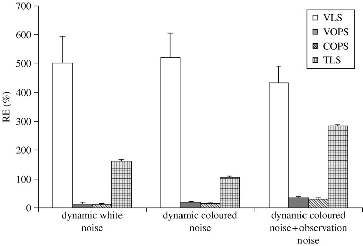
The above process was examined under three different noise scenarios: (i) dynamic white noise, (ii) dynamic coloured noise and (iii) dynamic coloured and observation white noise. For the dynamic white noise case, ϵ_x and ϵ_y are independent Gaussian white noise with zero mean and variance=0.16. Dynamic coloured noise is generated by the following: , where e(n)=[e_x(n) e_y(n)]^T, and e_x and e_y are independent Gaussian white noise with zero mean and variance=0.16. The results are provided in figure 3. Under all noise cases, the results show that the averages and variances of RE computed from the VOPS and COPS are statistically smaller than the results computed from the TLS and VLS.

Figure 3.

Comparison of RE values for all algorithms compared in example 1. ANOVA was performed (α=0.05). There are significant differences in every case (p<0.0001). Student–Newman–Keuls test was performed (α=0.05). Under all noise cases, the RE values are in the order COPS=VOPS<TLS<VLS.

(ii) Example 2

For the second simulation example, we consider another two-channel VNAR process provided by the following:

(4.5)

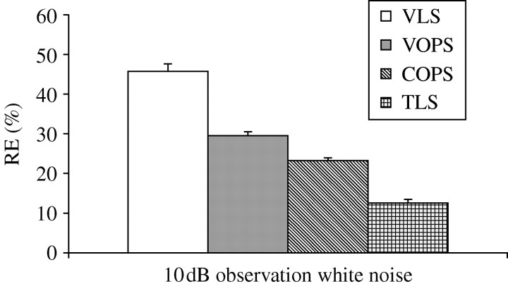
The above equation describes the well-known Henon map (Henon 1976). To the Henon map, 10 dB observation white noise was added. REs of the four methods are shown in figure 4. The TLS approach provides the best parameter estimates followed by the COPS, VOPS and VLS.

Figure 4.

Comparison of RE values for all algorithms considered in example 2. ANOVA was performed (α=0.05). There are significant differences (p<0.0001). Student–Newman–Keuls test was performed (α=0.05). Under the 10 dB observation white noise case, the RE values are in the order TLS<COPS<VOPS<VLS.

In summary, the comparative results show that both the VOPS or COPS algorithms are, in general, far superior to the VLS for all types of noise and they are superior to the TLS for dynamic noise. The TLS provides better results followed by the VOPS, COPS and VLS when the system is corrupted by observation noise provided that it uses the accurate model order selection criterion (e.g. optimal parameter search; Lu et al. 2001).

5. Sensitivity analysis

Models based on physiological knowledge and first principles attempt to identify functional details about the system under study. This approach represents a second general avenue for investigating the complex functional interactions of the complex control loops of the cardiovascular system (CVS). A prime example is the human baroreflex system, which relies on both arterial and cardiopulmonary sensors for information on the state of the system to stabilize blood pressure via various combinations of changes in heart rate, heart contractility, systemic resistance and venous capacitance (see Batzel et al. 2006). In this approach, model equations represent the interaction of states, and parameters reflect the individual response characteristics of the system in a particular subject. Hence, parameter estimation can be critical for model validation, subject classification and patient diagnosis. In this section, the contribution of SA in parameter identification is described, as well as its relevance for addressing the problem of restrictions on the data such as (i) the collection by non-invasive measurements and (ii) cost constraints such as are typically seen in the clinical setting where accurate model adaptation to the individual is vital. The importance of SA is especially evident for nonlinear system identification since the model terms grow exponentially with increasing order of nonlinearity. SA seeks to strategically reduce the number of model parameters to be estimated without sacrificing model usefulness.

Parameter sensitivity will be described in terms of the following typical model system:

(5.1)

where represents the states of the system; represents the observations; and represents the parameter vector. Parameter estimation is normally carried out with respect to a cost functional J(p) and the data ξ_i collected at times t_i, 1≤i≤s.

(a) Definitions of identifiability and sensitivity analysis

Various definitions of model identifiability can be found in Cobelli & DiStefano (1980) such as structural identifiability (or least-squares identifiability) defined in terms of the local minimum of the cost functional used in estimation and output distinguishability related to the ability to distinguish outputs when parameters are perturbed. This section focuses on sensitivity identifiability of system (5.1) using the following relations:

(5.2)

The matrix S (time dependent) is called the sensitivity matrix. Note that the three definitions of identifiability can be shown to be equivalent (see Cobelli & DiStefano 1980). SA refers broadly to methods for assessing the relationships between model output, parameter values (and estimation) and data sources. System (5.1) is said to be sensitivity identifiable if relation (5.2(ii)) can be solved uniquely for a given Δp, which is true if and only if rank (S)=r or equivalently det . The matrix S will be a building block in the methods discussed below, and under suitable conditions the noise in the measured data can be related to the Fisher information matrix. Applications of SA include (i) model reduction, (ii) improvement in computational efficiency, and (iii) experimental design. Three important techniques for SA, classical sensitivity, subset selection and generalized sensitivity, will be presented. Using information derived from these techniques, the set of parameters to be estimated may be reasonably reduced and experimental design improved. For examples of such analysis, see Heldt et al. (2006) and Fink et al. (2008).

What can be referred to as classical SA examines how parameter changes influence model output. Each element in the sensitivity matrix S describes how a single output varies with a single parameter. For simplicity, consider the relationship between a single real-valued output y and single real-valued parameter p, so that y=y(p) and p is in some open interval I, where we assume that y is differentiable on I. Consider a fixed and assume that and . Corresponding to Δp with , we define and consider the relative variations (Δp/p₀) and (Δy/y₀). The sensitivity σ of y with respect to p at p₀ is defined as .

Relative variations weight the responses and render 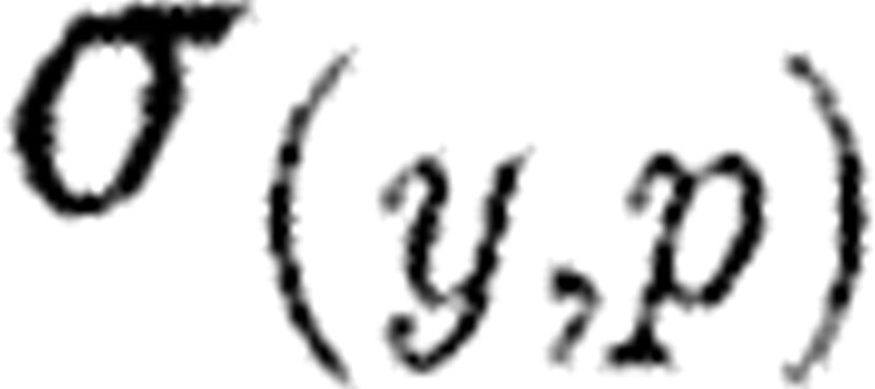invariant under change of units in p or y. Sensitivities are defined at each time point and the resulting sensitivity functions in S trace output sensitivities with respect to particular parameters over time. These sensitivity functions can be found by appending model (5.1) with additional differential equations for the individual sensitivities in S as variables and then solving the extended system (see Fink et al. (2008) including discussion of initial conditions). The resultant sensitivities can detect those parameters whose variation have least impact on model output and perhaps can be reasonably estimated from the literature and not through some estimation procedure.

(b) Subset selection

Subset selection is a second SA method that can be applied, for example, in the least-squares estimation problem with the cost of the form given in equation (5.1) (see Vélez-Reyes & Verghese 1995; Burth et al. 1999). Using a gradient-based method to update a current guess p_c of the parameter vector, we define the new guess p_n by , where Δp is the correction term satisfying the update relation

and as before ξ_i is a measurement at time t_i. Now, is essentially the sensitivity matrix S given in equation (5.2(i)) but where model predictions at various times 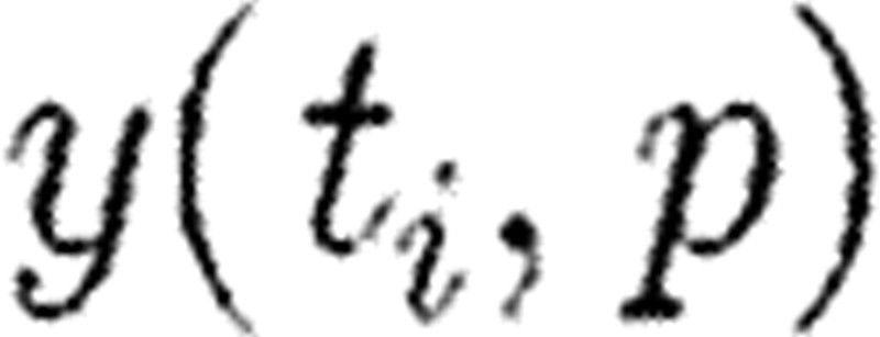are incorporated. Such an update algorithm fails when is singular. Note that is evaluated at fixed nominal parameter values (normalized) and thus provides only a local analysis of the feasibility of parameter identification.

Subset selection described in Burth et al. (1999) uses QR factorization with column pivoting to carry out a partition of the matrix so that the first j columns of are (‘most’) linearly independent and the remaining columns are dependent or nearly so as measured by the magnitude of the associated eigenvalues. This procedure also naturally associates parameters with eigenvalues. A new update on estimation is only applied to the j parameters associated with the first j linearly independent columns, while the remaining parameters are fixed at the current estimate. Numerical considerations can be used to sort parameters by the magnitude of associated eigenvalues allowing for a further refinement in the analysis of which parameters are likely to be reasonably estimated. Only those parameters associated with larger eigenvalues would be deemed estimatable. Zero eigenvalues indicate a set of interdependent parameters not uniquely identifiable. For techniques to analyse this problem and extract from the parameter set a subset that will in principle be identifiable see Catchpole et al. (1998), Gimenez et al. (2004) and Fink et al. (2008).

(c) Generalized sensitivities

Generalized sensitivity functions (GSFs) introduced by Thomaseth & Cobelli (1999) provide information on the relevance of measurements of output variables of a system for the identification of specific parameters (sensitivity of parameter estimates with respect to measurements). Consider system (5.1) as a single output system and the data given at time points t_k in a time interval 0≤t≤T with parameter vector p, and f sufficiently smooth. At time t_k we assume the measurement ξ_k=Z(t_k)+e_k for k=1, …, M, where Z(t_k) is the ‘true’ output of the system and e_k is the measurement noise. Noise functions are assumed to have zero mean and to be identically distributed with variances σ_k independent of p. A generalized sensitivity function 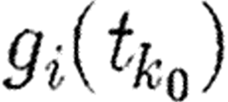with respect to the parameter component p_i of p at the time instant 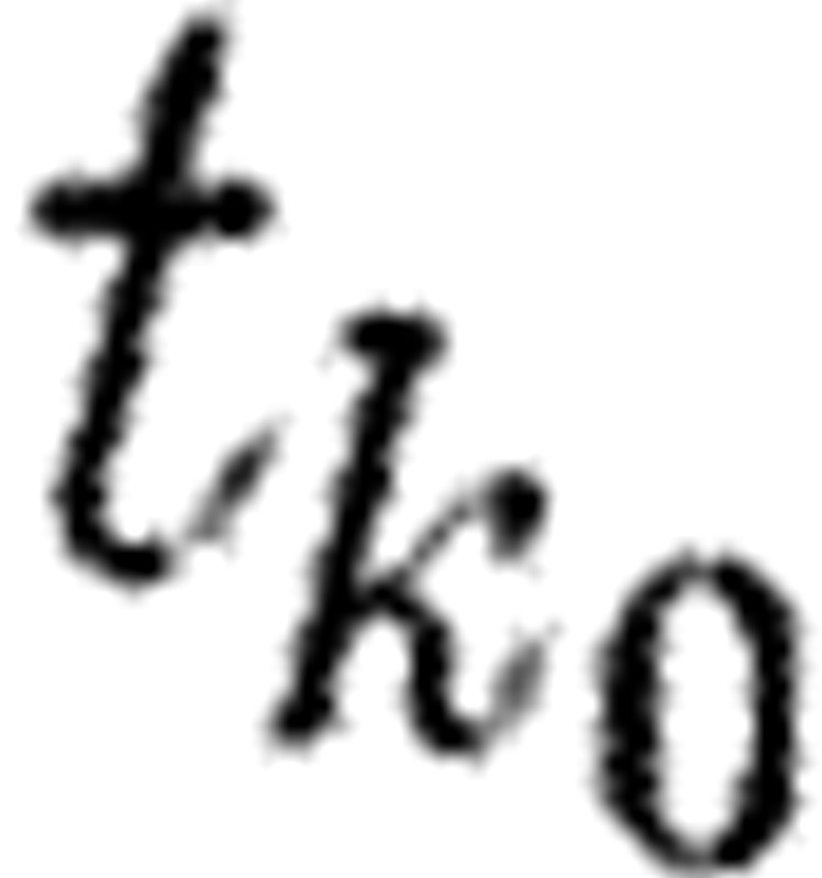for p in a neighbourhood of p₀ (an assumed true parameter for the data) is given by (compare (5.2))

Note that the gradients in the above equation incorporate information of the sensitivity matrix (see Batzel et al. 2006). Given the parameter vector p, each GSF g_i provides information on the correlation between the given parameter p_i and other parameters with respect to the output measurements.

Non-monotonic behaviour of g_i indicates that the information in the measurements is correlated with other parameters while monotonic behaviour indicates freedom from correlation. GSF also indicate the data intervals most relevant for the parameter estimation process: the intervals where the rise from 0 to 1 (beginning and ending values of the GSF) occurs are the intervals most relevant. Clearly, GSFs can provide valuable information on experimental design for data collected in the clinical setting restricted by clinical constraints.

(d) Applications of sensitivity analysis

The above three methods can be applied jointly to devise an effective parameter estimation protocol by using the methods to (i) detect which parameters are numerically reliably identifiable (subset selection), (ii) detect parameters whose variation does not greatly impact model output and hence can be reasonably estimated from literature, group or allometric estimation (classical SA), and (iii) design efficient data collection (generalized SA).

6. Conclusion

In this work, several methodologies have been shown each approaching the complexity of CVV and CV function from different points of view. Also, the application examples concern various data subsets, conditions and addressed parts of a multifaceted system. Despite the vast physiological knowledge of the CV and neural systems involved, tailoring of methods and models to specific applications is still needed. In this perspective, three main trends have been presented and discussed in the present review, which aim at providing efficient tools in reducing the CV regulation complexity: (i) introducing a priori haemodynamic knowledge with suitable grey-box modelling, (ii) describing nonlinear elements in order to improve the goodness of fit and reduce the required parameters, and (iii) assessing the relative importance of modelling features by SA. Consistent progress can be foreseen by the application and further integration of these methods in suitable models and computational tools.

References

- Akselrod S, Gordon D, Ubel F.A, Shannon D.C, Berger A.C, Cohen R.J.1981Power spectrum analysis of heart rate fluctuation: a quantitative probe of beat-to-beat cardiovascular control. Science. 213, 220–222. 10.1126/science.6166045. [DOI] [PubMed] [Google Scholar]
- Baselli G, et al. 1994A model for the assessment of heart period and arterial pressure variability interactions and of respiration influences. Med. Biol. Eng. Comput. 32, 143–152. 10.1007/BF02518911. [DOI] [PubMed] [Google Scholar]
- Batzel J.J, Kappel F, Tran H.T, Schneditz D.Cardiovascular and respiratory systems: modeling, analysis, and control. In SIAM 2006Philadelphia, PA:SIAM [Google Scholar]
- Burth M, Verghese G.C, Vélez-Reyes M.1999Subset selection for improved parameter estimation in on-line identification of a synchronous generator. IEEE Trans. Power Syst. 14, 218–225. 10.1109/59.744536. [DOI] [Google Scholar]
- Catchpole E.A, Morgan B.J.T, Freeman S.N.1998Estimation in parameter redundant models. Biometrika. 85, 462–468. 10.1093/biomet/85.2.462. [DOI] [Google Scholar]
- Chen X, Mukkamala R.2008Selective quantification of the cardiac sympathetic and parasympathetic nervous systems by multi-signal analysis of cardio-respiratory variability. Am. J. Physiol. 294, H362–H371. [DOI] [PubMed] [Google Scholar]
- Chen X, Kim J, Sala-Mercado J.A, Hammond R.L, Elahi R.I, Scislo T, Swamy G, O'Leary D.S, Mukkamala R.2008Estimation of the total peripheral resistance baroreflex impulse response from spontaneous hemodynamic variability. Am. J. Physiol. 294, H293–H301. 10.1152/ajpheart.00852.2007. [DOI] [PubMed] [Google Scholar]
- Chon K.H, Mullen T.J, Cohen R.J.1996A dual-input nonlinear system analysis of autonomic modulation of heart rate. IEEE Trans. Biomed. Eng. 43, 530–544. 10.1109/10.488800. [DOI] [PubMed] [Google Scholar]
- Cobelli C, DiStefano J.J., III1980Parameter and structural identifiability concepts and ambiguities: a critical review and analysis. Am. J. Physiol. 239, R7–R24. [DOI] [PubMed] [Google Scholar]
- Fink M, Batzel J.J, Tran H.T.2008A respiratory system model: parameter estimation and sensitivity analysis. Cardiovasc. Eng. 8, 120–134. 10.1007/s10558-007-9051-7. [DOI] [PubMed] [Google Scholar]
- Geweke J.1982Measurement of linear dependence and feedback between multiple time series. J. Am. Stat. Assoc. 77, 304–313. 10.2307/2287238. [DOI] [Google Scholar]
- Gimenez O, Viallefont A, Catchpole E.A, Choquet R, Morgan B.J.T.2004Methods for investigating parameter redundancy. Anim. Biodiv. Conserv. 27, 561–572. [Google Scholar]
- Granger C.W.J.1963Economic processes involving feedback information and control. Inform. Control. 6, 28–48. 10.1016/S0019-9958(63)90092-5. [DOI] [Google Scholar]
- Guyton A.C, Harris J.W.1951Pressoreceptor-autonomic oscillation; a probable cause of vasomotor waves. Am. J. Physiol. 165, 158–166. [DOI] [PubMed] [Google Scholar]
- Heldt, T., Long, B., Verghese, G. C., Szolovits, P. & Mark, R. G. 2006 Integrating data, models, and reasoning in critical care. In Engineering in Medicine and Biology Society, 2006 EMBS 28th Annu. Int. Conf. of the IEEE, vol. 1, pp. 350–353. [DOI] [PubMed]
- Henon M.1976A two-dimensional map with strange attractor. Commun. Math. Phys. 50, 69–77. 10.1007/BF01608556. [DOI] [Google Scholar]
- Hyndman B.W, Kitney R.I, Sayers B.M.1971Spontaneous rhythms in physiological control systems. Nature. 233, 339–341. 10.1038/233339a0. [DOI] [PubMed] [Google Scholar]
- Koepchen H.P.History of studies and concepts of blood pressure waves. In Mechanisms of blood pressure waves Miyakawa K, Koepchen H.P, Polosa C.1984. pp. 3–27. Eds. New York, NY:Springer. [Google Scholar]
- Levy M.N.1971Sympathetic–parasympathetic interactions in the heart. Circ. Res. 29, 437–445. [DOI] [PubMed] [Google Scholar]
- Ljung L.System identification: theory for the user. In Prentice-Hall 1999Englewood Cliffs, NJ:Prentice-Hall [Google Scholar]
- Lu S, Ju K, Chon K.H.2001A new algorithm for linear and nonlinear ARMA model parameter estimation using affine geometry. IEEE Trans. Biomed. Eng. 48, 1116–1124. 10.1109/10.951514. [DOI] [PubMed] [Google Scholar]
- Moon T.K, Stirling W.C.Mathematical methods and algorithms for signal processing. In Prentice Hall 2000Upper Saddle River, NJ:Prentice Hall [Google Scholar]
- Mukkamala R, Toska K, Cohen R.J.2003Noninvasive identification of the total peripheral resistance baroreflex. Am. J. Physiol. 284, H947–H959. [DOI] [PubMed] [Google Scholar]
- Mukkamala R, Kim J, Li Y, Sala-Mercado J, Hammond R.L, Scislo T, O'Leary D.S.2006Estimation of arterial and cardiopulmonary total peripheral resistance baroreflex gain values: validation by chronic arterial baroreceptor denervation. Am. J. Physiol. 290, H1830–H1836. 10.1152/ajpheart.00898.2005. [DOI] [PubMed] [Google Scholar]
- Porta G, Aletti F, Vallais F, Baselli G.2009Multimodal signal processing for the analysis of cardiovascular variability. Phil. Trans. R. Soc. A. 367, 391–409. 10.1098/rsta.2008.0229. [DOI] [PubMed] [Google Scholar]
- Saul J.P, Berger R.D, Chen M.H, Cohen R.J.1989Transfer function analysis of autonomic regulation. II. Respiratory sinus arrhythmia. Am. J. Physiol. 256, H153–H161. [DOI] [PubMed] [Google Scholar]
- Thomaseth K, Cobelli C.1999Generalized sensitivity functions in physiological system identification. Ann. Biomed. Eng. 27, 607–616. 10.1114/1.207. [DOI] [PubMed] [Google Scholar]
- Vélez-Reyes, M. & Verghese, G. C. 1995 Subset selection in identification, and application to speed and parameter estimation for induction machines. In Proc. 4th IEEE Conf. on Control Applications, pp. 991–997.
- Wang H, Ju K, Chon K.H.2007Closed-loop nonlinear system identification via the vector optimal parameter search algorithm: application to heart rate baroreflex control. Med. Eng. Phys. 29, 505–515. 10.1016/j.medengphy.2006.06.013. [DOI] [PubMed] [Google Scholar]
- Xiao X, Mukkamala R, Sheynberg N, Grenon S.M, Ehrman M.D, Mullen T.J, Ramsdell C.D, Williams G.H, Cohen R.J.2004Effects of simulated microgravity on closed-loop cardiovascular regulation and orthostatic intolerance: analysis by means of system identification. J. Appl. Physiol. 96, 489–497. 10.1152/japplphysiol.00602.2003. [DOI] [PubMed] [Google Scholar]
- Xiao X, Mullen T.J, Mukkamala R.2005System identification: a multi-signal approach for probing neural cardiovascular regulation. Physiol. Measure. 26, R41–R71. 10.1088/0967-3334/26/3/R01. [DOI] [PubMed] [Google Scholar]
- Zou R, Wang H, Chon K.H.2003A robust time-varying identification algorithm using basis functions. Ann. Biomed. Eng. 31, 840–853. 10.1114/1.1584683. [DOI] [PubMed] [Google Scholar]