M³: an improved SNP calling algorithm for Illumina BeadArray data

Abstract

Summary: Genotype calling from high-throughput platforms such as Illumina and Affymetrix is a critical step in data processing, so that accurate information on genetic variants can be obtained for phenotype–genotype association studies. A number of algorithms have been developed to infer genotypes from data generated through the Illumina BeadStation platform, including GenCall, GenoSNP, Illuminus and CRLMM. Most of these algorithms are built on population-based statistical models to genotype every SNP in turn, such as GenCall with the GenTrain clustering algorithm, and require a large reference population to perform well. These approaches may not work well for rare variants where only a small proportion of the individuals carry the variant. A fundamentally different approach, implemented in GenoSNP, adopts a single nucleotide polymorphism (SNP)-based model to infer genotypes of all the SNPs in one individual, making it an appealing alternative to call rare variants. However, compared to the population-based strategies, more SNPs in GenoSNP may fail the Hardy–Weinberg Equilibrium test. To take advantage of both strategies, we propose a two-stage SNP calling procedure, named the modified mixture model (M³), to improve call accuracy for both common and rare variants. The effectiveness of our approach is demonstrated through applications to genotype calling on a set of HapMap samples used for quality control purpose in a large case–control study of cocaine dependence. The increase in power with M³ is greater for rare variants than for common variants depending on the model.

Availability: M³ algorithm: http://bioinformatics.med.yale.edu/group.

Contact: name@bio.com; hongyu.zhao@yale.edu

Supplementary information: Supplementary data are available at Bioinformatics online.

1 INTRODUCTION

Genome-wide association studies (GWAS) have resulted in the discovery of numerous genetic variants contributing to major human diseases (Klein et al., 2005; Sladek et al., 2007; The Wellcome Trust Case Control Consortium, 2007). These studies benefit from the success of the International HapMap Project in cataloging and characterizing millions of single nucleotide polymorphisms (SNPs) for the purpose of GWAS (The International HapMap Consortium, 2007). Another major contributing factor is the availability of high-density and low-cost SNP arrays, such as those from Affymetrix and Illumina, which allow researchers to genotype millions of SNPs.

For any microarray genotyping platform, an accurate genotyping algorithm is needed to convert the observed probe intensities into genotypes, and many methods have been proposed for SNP calling. For example, RLMM (Rabbee and Speed, 2005), BRLMM (AFFYMETRIX, 2006) and CHIAMO (Chierici et al., 2010; Marchini et al., 2007) have been developed for the Affymetrix GeneChip, and Iluminus (Teo et al., 2007), GenoSNP (Giannoulatou et al., 2008) and GenCall (Illumina Inc., 2005, 2009) for the Illumina BeadArray. In addition, some algorithms are applicable to both platforms, such as CRLMM (Carvalho et al., 2007; Ritchie et al., 2009) and BEAGLE with BEAGLECALL (Browning and Yu, 2009). In this article, we focus on the Illumina platform.

With green–red color single-base extension biochemistry (Steemers et al., 2006), Illumina microarrays use allele signal intensity to measure two alleles, A and a, at each SNP for every individual. One class of calling algorithms considers data from all study subjects for one SNP at a time. We call these algorithms the population-based ones. Their basic premise is that the three possible genotypes from an SNP with alleles A and a, namely AA, Aa and aa, will form three distinct clusters and each individual's genotype can be inferred from its cluster membership. However, this approach requires every cluster to contain a sufficient number of individuals to be correctly inferred, so that a large number of samples are needed if the minor allele frequency (MAF) of an SNP is low. In practice, three genotype clusters of a fraction of SNPs may be shifted away from their expected positions (Giannoulatou et al., 2008; Teo et al., 2007), which will lead to a genotyping error rate of ~1% from missing genotypes or miscalled genotypes (Browning and Yu, 2009).

Another algorithm, GenoSNP, is distinguished from the population-based algorithms in that it genotypes all SNPs within one individual at a time under the assumption that probes for different SNPs have similar response features across the genome (Giannoulatou et al., 2008). That is, instead of genotyping SNP-by-SNP, this algorithm infers genotypes of all the SNPs for every individual in turn. We refer to this algorithm as the SNP-based strategy. Since genotypes are called at the individual level and the variation within a cluster may be smaller than that between clusters, there is no need to collect a large number of samples to achieve high accuracy of genotype calls for low MAF SNPs. However, compared with the population-based strategy, many more SNPs fail the Hardy–Weinberg Equilibrium (HWE) test using this algorithm, suggesting a possible violation of the assumption that all the SNPs behave similarly across the genome.

To take advantage of both the population-based and the SNP-based calling approaches, in this article, we propose a two-stage SNP calling procedure without a reference population for the Illumina BeadArray platform. We call this procedure the ‘modified mixture model’ (M³). Generally, this method integrates the population-based strategy, e.g. GenCall, with the SNP-based genotyping algorithm, e.g. GenoSNP, to improve call accuracy for both common and rare variants. M³ is evaluated through comparison with other genotyping algorithms for Illumina mciroarray data.

2 STATISTICAL METHODS

2.1 Illumina Chip data description

We first describe the features of the Illumina data before introducing our method. In its probe design, the Illumina array is composed of many beadpools that consist of hundreds of thousands of beadtypes. With the dual-color single base extension biochemistry, each bead accommodates a 50mer probe sequence to hybridize near the beadtype site (Steemers et al., 2006), and 20 beads on average for each beadtype provide 20 pairs of allele-specific intensities for each DNA sample. Thus, each beadtype assaying two SNP alleles represents an SNP. In our study, the pair of raw intensities at each SNP for every individual are measured, and clusters of genotypes are inferred based on these measured intensities.

2.2 Model

Let x_jk=(r_jk, g_jk) denote the pair of raw intensities at the j-th SNP for the k-th individual, and its distribution is modeled as a four-component Gaussian mixture model (McLachlan and Peel, 2000). In fact, each measurement x_jk can be considered as arising from one of these components with probability π_ji, where i = 1, 2, 3 or 4. While performing SNP calling, the first three components in the mixture model correspond to three genotypes (AA, Aa and aa), and the last one is the null component with zero mean and large variance. The indicator variable z_jk, where z_jk = 1, 2, 3 or 4, denotes the latent genotype class for the j-th SNP of the k-th subject. Given the above notations, the complete likelihood function for the observed data is given by,

(1)

where k=1,…,n_j, j=1,…,S, n_j is the total number of individuals observed for the j-th SNP, and S is the total number of SNPs. Given the j-th SNP, x_j=(x_j1, x_j2,…, x_jnj) collects the raw intensities for all individuals, and Θ_j=(π_j, μ_j, Σ_j) denotes the unknown parameters of the Gaussian mixture model where π_j=(π_j1, π_j2, π_j3, π_j4), μ_j=(μ_j1, μ_j2, μ_j3, μ_j4) and Σ_j=(Σ_j1, Σ_j2, Σ_j3, Σ_j4). These parameters correspond to three genotype clusters and the null component in the model. Function Φ denotes the normal density at x_jk with mean μ_ji and variance–covariance matrix Σ_ji. We also assume that the latent variable z_jk follows the multinomial distribution.

We can find the maximum likelihood estimates (MLEs) of these parameters through solving the following score equation:

(2)

In practice, we estimate these parameters through the following Expectation Maximization (EM) algorithm (McLachlan and Peel, 2000).

The E (Expectation) step calculates the conditional expectation of Equation (1), given the observed pair of raw intensities x_j. When the current estimates are Θ_j^t for Θ_j in the t-th iteration, the conditional expectation of the log likelihood function is

(3)

Since the log likelihood function is a linear function of the unobservable indicator variable z_jk (McLachlan and Peel, 1999), replacing z_jk in the above conditional expectation equation will affect the E-step. At the (t+1)-th iteration, z_jk=i (i=1, 2, 3 or 4) is inferred by

(4)

The parameters of the normal components are estimated in the M (Maximization) step. The iterative estimates for the mean μ_ji and variance–covariance matrix Σ_ji are

(5)

(6)

Note the parameters can be estimated by gmm package in MatLab (MathWorks, 2009).

After the above EM algorithm converges, the conditional probability that the pair of intensities (x_jk) belong to the i-th cluster is inferred as the Posterior Rate (PR: p_jkⁱ), which can be estimated through the Bayes Theorem,

(7)

where P(x_jk|i) refers to the likelihood of x_jk if it belongs to the i-th cluster with mean μ_ji and variance–covariance Σ_ji, and π_ji is the probability of the i-th cluster for the j-th SNP. This measure, PR, is closely related to the SNP calling result, that is, a larger value of PR implies a higher quality of the inferred genotype. Thus, the PR can be used to identify the observations with strong signals of clusters. Based on the PR, the average posterior rate (APR) for the j-th SNP (p_j) is defined by,

(8)

Note that the APR is one important criterion applied in the second stage of our two-stage SNP calling procedure to select good-quality SNPs, and n_jⁱ is the total number of observations within the j-th SNP for the i-th cluster.

For the X chromosome, male samples are only called as homozygote genotypes, and their calling strategy is quite different from that of female samples. It might greatly influence the call accuracy if we ignore the gender information in the model. Thus, a gender-dependent model (M_dep³) containing two calling algorithms is developed for female and male subjects, separately. This model contains a four-component model (major homozygote, heterzygote, minor homozygote and the null component) for female individuals and a three-component model (two homozygotes and the null component) for male individuals. Then the relevant APR of each SNP is the average value of the APR calculated from the female samples and APR from the male samples.

2.3 Two-stage SNP calling procedure

The two-stage genotyping procedure for SNP calling is designed to integrate the population-based strategy implemented in GenCall and the SNP-based approach implemented in GenoSNP. In the first stage, a Gaussian mixture model is used to call each SNP in turn across the whole genome. This step is a population-based calling method. In the second stage, a union set of SNPs with low MAFs (e.g. MAF < 0.05) and poor APR (e.g. APR < 0.9) are selected, and each selected SNP is re-called with the assistance of a reference SNP that can provide additional information about shapes, centers and boundaries of the clusters. This second stage is very much in the same spirit as GenoSNP to borrow information across SNPs, but it focuses more on poorly behaving SNPs where calling can be improved by means of incorporating information from good-quality SNPs.

In our procedure, we choose to apply a population-based strategy in the first stage. Empirical evidence suggests that a large proportion of SNPs with high MAF can be more reliably called than those from a SNP-based strategy, because it has been noted that genotype clusters may differ among the SNPs (Giannoulatou et al., 2008; Teo et al., 2007). Therefore, the population-based strategy is preferable for common SNPs. However, as an increasing number of SNPs are included on a genotyping microarray with a deliberate emphasis on rare variants, the population-based approach may not be optimal. As we mentioned in Section 1, a very large number of individuals are required to ensure that at least one subject is observed in each of the three genotype classes, and a certain number of individuals within each cluster are needed to ensure a precise estimate of distribution parameters for every cluster. In this context, the SNP-based approach, GenoSNP, is more appealing. However, this approach depends on two critical assumptions: (i) different probes have the same response features on the array; and (ii) the variation within a cluster is smaller than that between clusters. Similar assumptions are required for the second stage analysis of our method, namely that the poor-quality SNP and the reference SNP have similar patterns, and the within-cluster variation is less than that between clusters (Giannoulatou et al., 2008).

2.4 Reference SNP selection

A very important component of our proposed procedure is to find an appropriate reference SNP to improve SNP calling accuracy of SNPs that are difficult to call accurately on their own. To achieve this objective, a three-step selection procedure is proposed below. Throughout this section, we use ‘testing SNPs’ to denote SNPs that need to be re-called (that is, to have their calling accuracy improved) and ‘reference SNPs’ to denote good-quality SNPs.

• Step I: selecting SNPs with high APR as candidate reference SNPs. In the first stage, the APR of one SNP is defined as the average value of PR of all subjects for one SNP. We have found that SNPs with a lower MAF tend to have a smaller APR than more common ones, so the MAF of an SNP is highly correlated with its APR. In real data analysis, SNPs having a large APR near the testing SNP are selected to be the candidate reference SNPs. We call these SNPs as Ref-1 SNPs.

• Step II: selecting SNPs with good clustering properties from Ref-1 SNPs. Although Ref-1 SNPs have a large APR, some of them may not have high-quality clusters. The shapes, centers and boundaries of three clusters for these Ref-1 SNPs may not provide precise distribution parameters of each cluster as a reference. At the second step, Ref-1 SNPs with each cluster containing at least 10% of samples are further selected, denoted as Ref-2 SNPs.

• Step III: measuring the similarity between the testing SNP and each Ref-2 SNP. We consider three possible criteria to select a reference SNP in this step.

1. Calculating the APR of each aggregated dataset formed by the testing SNP with each Ref-2 SNP in turn. For example, an aggregated dataset of size ((n_c+n_d) × 1) is made up of the c-th testing SNP (n_c × 1) and d-th reference SNP (n_d × 1). The relevant APR of this aggregated data is given by

   (9)

   where p_jkⁱ is defined by Equation (7). We select the Ref-2 SNP that gives the largest APR (p_d^*, d=1,…,t_c, t_c is the total number of Ref-2 SNPs for the cth testing SNP) for this aggregated dataset.

2. Calculating the Mahalanobis distance (McLachlan, 1999) between the testing SNP and each Ref-2 SNP, and the Ref-2 SNP with the minimum Mahalanobis distance value is selected. Generally, the Mahalanobis distance measures the overall similarity between two SNPs.

3. To explore the detailed resemblance of each cluster between the testing SNP and each Ref-2 SNP, we further introduce a measure, Cluster Distance (S_c), in the following to compare the clusters between two SNPs. Both the testing SNP and Ref-2 SNPs are classified into three clusters corresponding to three genotypes in the following form,

   

   (10)

   where y_jk is a simple projection function of x_jk. It transforms the 2D vector x_jk into a univariate variable y_jk without losing main clustering characteristics (Teo et al., 2007), and it is easy to group transformed intensity y_jk into three clusters in terms of Equation (10). Note that i^* denotes the index of clusters where y_jk falls inside the i^*th cluster and i^*=1, 2 or 3. u_j1 and u_j2 are used to divide the intensities y_j=(y_j1,…,y_jnj)^T of the j-th SNP into three genotype clusters with the following two steps.

1. y_j is roughly classified into different clusters, and at least three observations are in each cluster. In the first step, u_j1 and u_j2 are given by

   

2. Update u_j1 and u_j2 to find the optimum boundaries to identify distinct clusters.

If y_j is classified into three clusters with means μ_ji^* (i^*=1, 2 or 3) corresponding to three genotypes in the first step, u_j1 and u_j2 are further defined by,

If y_j is grouped into two clusters in the first step, u_j1 and u_j2 are given by,

If only one cluster is generated for y_j in the first step, u_j1 and u_j2 are not defined.

Once y_j is grouped into different clusters in an appropriate way, we define a measure (S_c), which quantifies the similarity of clusters between the c-th testing SNP and each Ref-2 SNP,

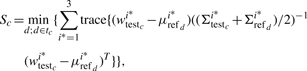(11)

where d=1,2,…,t_c and t_c is the total number of Ref-2 SNPs for the c-th testing SNP, w_testc^i* is the transformed intensity vector of the i^*th cluster at the c-th testing SNP, μ_refd^i* denotes the mean vector of the d-th Ref-2 SNP for the i^*th cluster, Σ_testc^i* and Σ_refd^i* are the variance–covariance matrices of the c-th testing SNP and d-th Ref-2 SNP, respectively. In general, S_c measures the minimum distance between the clusters of the c-th testing SNP and each Ref-2 SNP.

It is desirable to select one reference SNP so that the genotypes of the poor-quality SNP can be best called based on one of the three criteria discussed above. Figure 1 displays the comparison results between the testing SNP (rs1002189) and the reference SNP selected by each of the three methods, and shows that the three methods are ranked in the order of Average Posterior Rate < Mahalanobis Distance < Cluster Distance. The overall comparisons of three methods are evaluated in the Supplementary Materials. We note that this SNP is not a real testing SNP with low MAF, because the distinct performance of three methods, APR, Mahalanobis Distance and Cluster Distance, is difficult to show using low-frequency testing SNPs that may lack some clusters. Thus, we choose this common SNP to show the similarity between the testing SNP and the reference SNP. Throughout the following section, we use the third method (Cluster Distance) to choose the reference SNP for genotype calling on poor SNPs. Figure 2 also illustrates how the reference SNP can assist in accurate calling of three SNPs, rs10482982, rs1009925 and rs10154218, with low MAF. Although it is difficult to assign genotypes to some individuals at these three SNPs alone, we expect that better calls can be made with the help of the reference SNP.

Fig. 1.

The comparison plots of the reference SNP selected by three methods (APR, Maholanobis Distance and Cluster Distance) for improving the calling result of the same testing SNP (rs1002189).

Fig. 2.

Illustration of how the reference SNP assists the genotype calling of three low MAF SNPs using the Cluster Distance measure.

3 RESULTS

3.1 Dataset and SNP calling methods

We consider an Illumina Omni 1M dataset that consists of 3258 samples, and 141 out of 3258 samples were from 38 distinct HapMap samples with some individuals genotyped multiple times. The overall performance is evaluated by comparing the SNP calls for these HapMap samples by different methods to those available from the International HapMap Project database (The International HapMap Consortium, 2007). In this article, we focus on the 942 313 SNPs in the whole genome with the exception of the sex chromosome. The X chromosome SNPs (24 717) are analyzed alone. The null genotypes in the HapMap project are ignored. The performance of our proposed method, M³, and other existing calling algorithms is evaluated based on this Illumina dataset.

It has been demonstrated that the call rate and call accuracy of both GenoSNP and CRLMM are better than those of Illuminus when a small number of samples are collected (Ritchie et al., 2011). As for CRLMM, its implementation depends on the reference population and its calculation strongly hinges on computer configuration (Ritchie et al., 2011; Zhang et al., 2010). Based on these considerations, we compare M³ with GenCall as a representative of the population-based method and GenoSNP as the SNP-based method. For the Illumina GenCall approach, genotypes with good GenCall scores (GC score ≥ 0.15) are used as the inferred genotypes. As discussed earlier, GenoSNP is built on a SNP-based mixture model without a reference population to genotype every individual in turn, and this model may be good at genotyping rare variants. It calculates the posterior probability of each sample at a specific SNP, and we use a cut-off value of 85% to select SNPs and samples with good quality. Samples and SNPs having poor clustering properties (low posterior probability) are treated as missing data. As discussed in the model section, the two-stage M³ approach aims to take the advantage of GenCall and GenoSNP. We use the PR of 0.85 as a cut-off to filter samples at a particular SNP in our analysis, and a union set of SNPs with MAF < 0.05 and APR < 0.9 are selected to be re-called in the second stage of our proposed method.

3.2 Comparisons

We first evaluate the SNP calling results by evaluating the call rate of each method and the concordance among them. The call rate is defined as the ratio of genotypes passing the calling threshold to the total number of genotypes that need to be inferred. The concordance rate between two algorithms refers to the percentage of agreement of inferred genotypes between two algorithms. The relevant results are summarized in Table 1. In brief, there is high consistency among these three methods (M³, GenCall and GenoSNP) overall. But, there are some discrepancies among these three algorithms. We note that the major homozygote calls by GenCall are more frequently called heterozygote by M³ and M³ more likely genotypes null components by GenCall and GenoSNP (Supplementary Materials). This is partially due to the fact that M³ gives the largest call rate (99.64%), followed by GenoSNP (99.22%) and GenCall (98.16%) (Table 1).

Table 1.

The comparisons of call rate and concordance rate among GenCall, GenoSNP and M³

Algorithm 1	Algorithm 2	Call rate (%)		Concordance (%)
		Algorithm 1	Algorithm 2
GenCall	M3	98.16	99.64	99.87
GenoSNP	M3	99.22	99.64	99.64
GenCall	GenoSNP	98.16	99.22	99.80

The unit of call rate and concordance rate is percentage %; M³: the modified mixture model.

Since the true genotypes are unknown, the above concordance comparisons do not reveal which method performs better. In the following, we focus on the genotype calls of 141 out of 3258 samples from 38 distinct HapMap samples using the genotypes of these individuals obtained from the HapMap project as a gold standard in our comparisons. One issue in using the SNP calls from the HapMap data is differentiating the major allele between two alleles at an SNP. In our comparisons, we count the discrepancy in homozygote calls, denoted by E (Error), between each of the three algorithms and HapMap data, and vary the cut-off level at 1, 10 and 50 to remove SNPs with different major allele assignments between each of the three algorithms and HapMap data. With a more stringent threshold, e.g. E < 1, fewer SNPs with inconsistent major allele assignment are compared. The results are summarized in Table 2. We note that M³ has the best average call accuracy and average call rate by three criterions (GenCall, GenoSNP and M³) under all three E cut-offs, followed by GenoSNP and GenCall. For example, when the threshold level for E is set at 1, the highest call rate and the best SNP calling accuracy are achieved by M³ (99.77%, 99.23%), followed by GenoSNP (99.21%, 98.74%) and GenCall (98.03%, 97.87%). With a less stringent cutoff, fewer accurate genotypes by M³ are obtained with average call accuracy 99.20% at E < 10 and 99.11% at E < 50. This is likely due to more consistent major allele assignments with a more stringent cut-off. A similar trend also occurs for GenoSNP and GenCall when the E cut-off becomes increasingly stringent.

Table 2.

The comparisons of call rates and concordance on HapMap samples for overall SNPs

Criterion	E (Error)	Item	GenCall (%)	GenoSNP (%)	M3 (%)
GenCall, GenoSNP	< 50	Call rate	98.03	99.13	99.75
and M3		Accuracy	97.85	98.45	99.11
	< 10	Call rate	98.03	99.20	99.76
		Accuracy	97.87	98.68	99.20
	< 1	Call rate	98.03	99.21	99.77
		Accuracy	97.87	98.74	99.23

M³: the modified mixture model; call rate: the percentage of valid genotypes; accuracy: the percentage of consistent genotype; criterion: which algorithm is selected to count E values between this algorithm and HapMap project due to the mis-assignment of major allele. E: the average error caused by the mis-assignment of the major allele under three criterions, GenCall, GenoSNP and M³, and three E cutoffs, E < 50, 10 and 1 are set.

When more SNPs are added to the genotyping arrays, a larger proportion of the newly identified SNPs will have lower MAFs than those already on the arrays. It has been demonstrated that GenoSNP performs better than other algorithms in calling rare variants (Giannoulatou et al., 2008; Ritchie et al., 2011). Since M³ tries to take advantage of both the population-based strategy and the SNP-based approach, we expect it to perform well for rare SNPs. Table 3 summarizes the comparison results for SNPs with MAF < 0.1, 0.05 and 0.01. We use HapMap data from four populations to estimate the MAF for each SNP, because the 38 HapMap samples in our Illumina data come from JPT (116), CHB (139), YRI (209) and CEU (174). We calculate the MAF of each SNP by the weighted value of the MAF of each population. The weight of each population is determined by its population proportion in the 38 HapMap samples. In general, M³ yields the best SNP calling accuracy and highest call rate under three E cut-offs for SNPs with MAF < 0.1, 0.05 and 0.01. For SNPs with very small MAF (<0.01), M³ (98.47 ~98.77%) provides large average call accuracy by three criterions, followed by GenoSNP (97.80% ~98.10%), GenCall (96.11% ~96.43%). Overall, when considering both common and rare variants, M³ yields the best SNP calling among the three methods.

Table 3.

Comparisons of call rates and concordance on HapMap samples for rare variants

SNPs	E (Error)	Item	GenCall	GenoSNP	M3
MAF < 0.1	< 50	Call rate	97.79	99.11	99.67
		Accuracy	97.52	98.49	99.12
	< 10	Call rate	97.81	99.12	99.67
		Accuracy	97.57	98.54	99.16
	< 1	Call rate	97.84	99.13	99.68
		Accuracy	97.62	98.59	99.20
MAF < 0.05	< 50	Call rate	97.73	99.13	99.64
		Accuracy	97.42	98.44	99.00
	< 10	Call rate	97.74	99.14	99.64
		Accuracy	97.48	98.50	99.06
	< 1	Call rate	97.73	99.15	99.65
		Accuracy	97.54	98.56	99.11
MAF < 0.01	< 50	Call rate	96.64	99.04	99.56
		Accuracy	96.11	97.80	98.47
	< 10	Call rate	96.67	99.06	99.57
		Accuracy	96.29	97.98	98.65
	< 1	Call rate	96.71	99.08	99.58
		Accuracy	96.43	98.10	98.77

M³: the modified mixture model; call rate: the percentage of valid genotypes; accuracy: the percentage of consistent genotype; E: the average error caused by the mis-assignment of the major allele under three criterions, GenCall, GenoSNP and M³, and three E cutoffs, E < 50, 10 or 1 are set. The different values in parentheses indicate the number of SNPs whose MAFs are < 0.1, 0.05 or 0.01, respectively.

The HWE test (P<0.0001) is a commonly used criterion to examine the quality of genotype calling of each SNP. We compare different SNP calling algorithms based on the proportion of SNPs failing the HWE test. As mentioned above, our Illumina dataset includes 3258 individuals, consisting most of African-Americans (AA) and European-Americans (EA), who are either Hispanic or non-Hispanic. We perform the HWE test on these four populations separately. The results are summarized in Table 4. Since GenoSNP is a SNP-based calling algorithm that does not consider HWE in SNP calling, a large number of SNPs (50860, 14432, 63170 and 20342 corresponding to the four populations, respectively) failed the HWE test. In contrast, for GenCall, the population-based strategy, fewer SNPs (14447, 1450, 32209 and 2801 for the four populations, respectively) failed the HWE test. Since M³ is largely a population-based approach, it performs relatively well on the HWE test with quite fewer SNPs (27288, 5155, 44123 and 7631 for the four populations, respectively) failing. Therefore, M³ performs well at both calling rare variants and generating calls that are more likely to pass the HWE test.

Table 4.

Comparisons of HWE test among GenCall, GenoSNP and M³

Population	Num-Sample	Algorithm	No. of failed SNPs
AA I	2005	GenCall	14 447
		GenoSNP	50 860
		M3	27 288
AA II	83	GenCall	1450
		GenoSNP	14 432
		M3	5155
EA I	867	GenCall	32 209
		GenoSNP	63 170
		M3	44 123
EA II	158	GenCall	2801
		GenoSNP	20 342
		M3	7631

AA I: African-Americans not of Hispanic origin; AA II: African-Americans of Hispanic origin; EA I: European Americans not of Hispanic origin; EA II: European Americans of Hispanic origin; Num-Sample: the number of subjects within each population; Algorithm: three algorithms in this table, that is, GenCall, GenoSNP and M³; Num-Failed SNP: the number of SNPs fail the HWE test within each population.

The higher call rate and more accurate genotype calls of M³ may help to increase statistical power to detect disease-associated variants, especially those with low MAFs. To quantify the power gain, we compare the average power to detect disease-associated variants based on the three calling algorithms using the HapMap sample data [ASW (87) and CEU (174)]. We consider a case–control scenario for AA and EA separately and assume a similar genotyping characteristic for the collected data. We assume a disease prevalence of 0.05, and the relative risk λ varies from 1.5 to 4 under the multiplicative model. The allele frequencies are based on empirical data from the HapMap project. We consider the statistical significance level by Bonferroni correction (5×10⁻⁸), and fix the number of cases and controls for both populations (AA: case:control=1250:758; EA: case:control=749:239). The power to detect the risk alleles based on the correct calls for all individuals and all SNPs is measured as a standard. For the three calling algorithms, we assume that the observed allele frequencies at each SNP and the number of cases or controls are similar to those observed from the HapMap samples collected in our study. The power comparisons for the overall SNPs and rare SNPs are summarized in Figures 3 and 4, respectively. In brief, compared with GenCall and GenoSNP, M³ has the largest power for both common variants and rare variants in both populations. When the relative risk increases, we observe a larger improvement of M³ versus GenCall or GenoSNP. The ratio of M³ versus GenCall or M³ versus GenoSNP measures this improvement, and it has been found that the power of M³ increases 1.46% and 1.03% compared with GenCall for AA and EA, respectively. Similarly, the increase in power of M³ versus GenoSNP is ~ 0.12% and 0.16% for both populations. In particular, the improvement of M³ versus GenCall or GenoSNP for rare variants is more noticeable than that for common variants. (The increase in power of M³ versus GenCall: 1.84% and 1.12% for both populations; the increase in power of M³ versus GenoSNP: 0.43% and 0.34% for both populations.) In general, the power achieved by M³ is closer to the ideal power when the genotypes of all study subjects are correctly inferred.

Fig. 3.

The average power to detect risk alleles for overall SNPs by HapMap, GenCall, GenoSNP and M³. Red solid line: the ideal power measured by the HapMap project; blue dash line: the average power measured by the GenCall; purple dot line: the average power measured by GenoSNP; green dot dash line: the average power measured by M³; cutoff: 5×10⁻⁸.

Fig. 4.

The average power to detect risk alleles for less common SNPs by HapMap data, GenCall, GenoSNP and M³. Less common SNPs: the SNPs with MAF < 0.05; cutoff: 5×10⁻⁸.

We also evaluate the performance of three algorithms on the X chromosome SNPs. The average call accuracy is compared with the HapMap project calls under three E(Error) cutoffs, E < 50, 10 or 1. Table 5 summarizes the overall concordance result on the X chromosome among three algorithms. Again, M³ provides the best call rate and accuracy on the sex chromosome SNPs, compared with GenCall and GenoSNP. It has been demonstrated that the model incorporating the gender information will perform better than methods (GenCall and GenoSNP) ignoring this gender information (Ritchie et al., 2011). We further exam the gender-dependent model in M³, denoted as M_dep³, on the X chromosome. Compared with M³ without incorporating the gender information, a higher call accuracy is achieved by the model M_dep³ involving the gender information (Table 5). The higher call accuracy on the male subjects results in the great improvement of calls. We suggest that the X chromosome SNPs should be called separately using a gender-dependent model (M_dep³) in practice.

Table 5.

The comparisons of call rates and concordance on HapMap samples for X chromosome SNPs

Criterion	E (Error)	Item	GenCall (%)	GenoSNP (%)	M3 (%)	Mdep3 (%)
GenCall, GenoSNP,	< 50	Call rate	97.67	99.00	99.31	99.75
M3, Mdep3		Accuracy	97.38	98.41	98.65	99.60
	< 10	Call rate	97.77	99.01	99.32	99.76
		Accuracy	97.48	98.45	98.69	99.63
	< 1	Call rate	97.91	99.03	99.33	99.77
		Accuracy	97.63	98.49	98.72	99.65

M_dep³: the gender−dependent modified mixture model; M³: the modified mixture model; call rate: the percentage of valid genotypes; accuracy: the percentage of consistent genotype; criterion: which algorithm is selected to count E values between this algorithm and HapMap project due to the mis-assignment of major allele. E: the average error caused by the mis-assignment of the major allele under four criterions, GenCall, GenoSNP, M³ and M_dep³, and three E cutoffs, E < 50, 10 and 1 are set.

4 DISCUSSION

A number of algorithms have been developed and are commonly used for SNP calling of Illumina genotyping arrays. One general strategy is the population-based approach where each SNP is analyzed individually and the data from all the study subjects at this SNP are used to define genotype clusters for calling. Since the performance of these population-based methods (such as GenCall) depends on well-defined genotype clusters, a large reference population is needed to achieve good accuracy. However, with an increasing number of less common SNPs on the arrays, the calling accuracy may not be as high due to the lack of information needed to define each of the three possible genotype clusters well. GenoSNP is an SNP-based approach that addresses this challenge, but it relies on the critical assumption that all the SNP probes perform similarly. This assumption is certain to be violated in practice. As a result, many more SNP calls than population-based calls fail the HWE test (P < 0.0001). To exploit the advantage of these two separate approaches, we have proposed a two-stage SNP calling procedure to improve the call accuracy of rare variants while retaining the accurate results for common SNPs. In the first stage of our procedure, we use a mixture model to call every SNP in turn, and then focus on a small fraction of poor-quality SNPs in the second stage by borrowing information from one reference SNP that matches well with the characteristics of the poor-quality SNPs in the genome.

This two-stage approach, named the modified mixture model (M³), was tested on an Illumina dataset with 3258 samples. In general, we observed good agreement between the M³ calls and those from GenCall and GenoSNP. Using 141 out of 3258 samples from 38 distinct HapMap samples in our data that have been genotyped, we were able to investigate the accuracy of different methods using the genotypes reported by the International HapMap Project. Our results show that M³ provides the highest call rate and the best genotyping accuracy. M³ performs better than GenCall on rare variants and generated fewer SNP calls that fail the HWE test than GenoSNP. In addition, M³ can increase statistical power to detect disease-associated variants compared with GenCall and GenoSNP, especially for rare variants.

The essence of M³ is to integrate the population-based statistical model with the SNP-based strategy (GenoSNP), to yield good call accuracy and a high call rate at each SNP without requiring a large reference population, especially for rare variants. An important aspect of M³ is that it searches for the appropriate SNP to assist in calling a poor-quality SNP. In practice, it is computationally prohibitive to search the reference SNP across the whole genome, thus we proposed to select a reference SNP near the testing SNP. Under the Illumina chip design, each bead accommodates a 50mer probe sequence that is made up of A, T, C and G near the SNP (Steemers et al., 2006), and it has been shown that the larger proportion of CG in this probe sequence of one SNP leads to the stronger intensity signal at this SNP (Carvalho et al., 2007). Thus, incorporating this probe sequence in the reference SNP selection procedure may help to find the most appropriate reference SNP. Additionally, empirical results suggest that our proposed selection procedure may be effective and the assumption that probes have similar response characteristics may hold at least for some of the probes. However, when some probes selected as the testing SNPs produce unusual variation in probe responses, the reference SNP cannot provide good cluster information to be used with these poor SNPs. In studies where certain samples with known genotypes, e.g. the HapMap samples in our dataset, the explicit consideration of these gold-standard samples may also help in the selection of reference SNPs. Our proposed method is a data-driven approach. In the future, we may borrow HapMap data information about genotype clusters to improve the quality of genotype calling of the illumina data. It remains to be determined whether there are better ways to identify a reference SNP or whether to include more than one reference SNP in the second-stage analysis.

The efficiency of M³ is strongly dependent on the assumption of the homogeneity of probe measurements. Since this condition may not be satisfied for some SNPs, it is desirable to develop a statistical model without the second-stage analysis to achieve more accurate genotyping results for both common and rare variants. Moreover, M³ fits the Gaussian mixture model on the raw intensities that may violate the assumptions of this mixture model. Thus, an additional normalization step (Illumina Inc., 2005; Teo et al., 2007) can be added to remove outlier SNPs and normalize intensities at each SNP before performing cluster analysis. This algorithm focuses on the analysis of Illumina arrays, and applicability of this idea to Affymetrix is worth investigating.

REFERENCES

- AFFYMETRIX. Technical Report, White Paper. Santa Clara, CA: Affymetrix, Inc.; 2006. BRLMM: an improved genotype calling method for the GeneChip Human Mapping 500K Array Set. [Google Scholar]
- Browning B.L, Yu Z.X. Simultaneous genotype calling and haplotype phasing improves genotype accuracy and reduces false-positive associations for genome-wide association studies. Am. J. Hum. Genet. 2009;85:847–861. doi: 10.1016/j.ajhg.2009.11.004. [DOI] [PMC free article] [PubMed] [Google Scholar]
- Carvalho B., et al. Exploration, normalization, and genotype calls of high-density oligonucleotide SNP array data. Biostatistics. 2007;8:485–499. doi: 10.1093/biostatistics/kxl042. [DOI] [PubMed] [Google Scholar]
- Chierici M., et al. An interactive effect of batch size and composition contributes to discordant results in GWAS with the CHIAMO genotyping algorithm. Pharmacogenomics J. 2010;10:355–363. doi: 10.1038/tpj.2010.47. [DOI] [PubMed] [Google Scholar]
- Giannoulatou E., et al. GenoSNP: a variational Bayes within-sample SNP genotyping algorithm that does not require a reference population. Bioinformatics. 2008;24:2209–2214. doi: 10.1093/bioinformatics/btn386. [DOI] [PubMed] [Google Scholar]
- Illumina Inc. Illumina GenCall Data Analysis Software. TECHNOLOGY SPOTLIGHT. 2005 [Google Scholar]
- Illumina Inc. Improved Cluster Generation with Gentrain2. Technical Note: DNA Analysis. 2009 [Google Scholar]
- Klein R.J., et al. Complement factor H polymorphism in age-related macular degeneration. Science. 2005;308:385–389. doi: 10.1126/science.1109557. [DOI] [PMC free article] [PubMed] [Google Scholar]
- Marchini J., et al. A new multipoint method for genome-wide association studies by imputation of genotypes. Nat. Genet. 2007;39:906–913. doi: 10.1038/ng2088. [DOI] [PubMed] [Google Scholar]
- MATLAB (R2009a) MathWorks. Inc. http://www.mathworks.com/help/techdoc/rn/bro2uzv.html.
- McLachlan G.J., Peel D. Wiley Series in Probability and Statistics. New York: John Wiley; 2000. Finite Mixture Models. [Google Scholar]
- McLachlan G.J, Peel D. In Computing Science and Statistics. Vol. 30. Fairfax Station, Virginia: Interface Foundation of North America; 1999. Computing Issues for the EM Algorithm in Mixture Models; pp. 421–430. [Google Scholar]
- McLachlan G.J. Mahalanobis distance. Resonance. 1999;4:20–26. [Google Scholar]
- Rabbee N, Speed T.P. A genotype calling algorithm for Affymetrix SNP arrays. Bioinformatics. 2005;22:7–12. doi: 10.1093/bioinformatics/bti741. [DOI] [PubMed] [Google Scholar]
- Reich D.E., et al. Quality and completeness of SNP databases. Nat. Genet. 2003;33:457–458. doi: 10.1038/ng1133. [DOI] [PubMed] [Google Scholar]
- Ritchie M.E., et al. R/Bioconductor software for Illumina's Infinium whole-genome genotyping BeadChips. Bioinformatics. 2009;25:2621–2623. doi: 10.1093/bioinformatics/btp470. [DOI] [PMC free article] [PubMed] [Google Scholar]
- Ritchie M.E., et al. Comparing genotyping algorithms for Illumina's Infinium whole-genome SNP BeadChips. BMC Bioinformatics. 2011;12:68. doi: 10.1186/1471-2105-12-68. [DOI] [PMC free article] [PubMed] [Google Scholar]
- Sladek R., et al. A genomewide association study identifies novel risk loci for type 2 diabetes. Nature. 2007;445:881–885. doi: 10.1038/nature05616. [DOI] [PubMed] [Google Scholar]
- Steemers F.J., et al. Whole-genome genotyping with the single-base extension assay. Nat. Methods. 2006;3:31–33. doi: 10.1038/nmeth842. [DOI] [PubMed] [Google Scholar]
- Teo Y., et al. A genotype calling algorithm for the Illumina BeadArray platform. Bioinformatics. 2007;23:2741–2746. doi: 10.1093/bioinformatics/btm443. [DOI] [PMC free article] [PubMed] [Google Scholar]
- The International HapMap Consortium. A second generation human haplotype map of over 3.1 million SNPs. Nature. 2007;449:851–861. doi: 10.1038/nature06258. [DOI] [PMC free article] [PubMed] [Google Scholar]
- The Wellcome Trust Case Control Consortium. Genome-wide association study of 14 000 cases of seven common diseases and 3000 shared controls. Nature. 2007;447:661–678. doi: 10.1038/nature05911. [DOI] [PMC free article] [PubMed] [Google Scholar]
- Zhang L., et al. Assessment of variability in GWAS with CRLMM genotyping algorithm on WTCCC coronary artery disease. Pharmacogenomics J. 2010;10:347–354. doi: 10.1038/tpj.2010.27. [DOI] [PubMed] [Google Scholar]
Associated Data
This section collects any data citations, data availability statements, or supplementary materials included in this article.