Comparison of Clustering Methods for Investigation of Genome-Wide Methylation Array Data

Abstract

The use of genome-wide methylation arrays has proved very informative to investigate both clinical and biological questions in human epigenomics. The use of clustering methods either for exploration of these data or to compare to an a priori grouping, e.g., normal versus disease allows assessment of groupings of data without user bias. However no consensus on the methods to use for clustering of methylation array approaches has been reached. To determine the most appropriate clustering method for analysis of illumina array methylation data, a collection of data sets was simulated and used to compare clustering methods. Both hierarchical clustering and non-hierarchical clustering methods (k-means, k-medoids, and fuzzy clustering algorithms) were compared using a range of distance and linkage methods. As no single method consistently outperformed others across different simulations, we propose a method to capture the best clustering outcome based on an additional measure, the silhouette width. This approach produced a consistently higher cluster accuracy compared to using any one method in isolation.

Introduction

Determining the methylation status of tissues/cells provides an insight into one mechanism of epigenetic gene control. In “normal” cell states methylation of the cytosine residues in a CpG dinucleotide within 5′ CpG islands and their close proximity regions known as “shores” (Irizarry et al., 2009) is associated with loss of gene activity. However, inappropriate methylation can cause genome-wide effects. For example genome-wide hypomethylation leads to chromosomal instability and an increase in the frequency of DNA strand breaks (Schmutte and Fishel, 1999). Conversely inappropriate hypermethylation leads to specific gene silencing. Determining differential methylation in human samples has become a common approach in basic and clinical studies. Whilst single nucleotide resolution of methylation at each CpG is preferable, in a clinical setting a system allowing high throughput analysis of samples is required. High density arrays to detect differential methylation of specific cytosines have fulfilled this need for a high throughput and reproducible platform to compare tissues or samples (e.g., Banister et al., 2011; Cotton et al., 2011; Fackler et al., 2011; Fryer et al., 2011; Martino et al., 2011). Briefly this procedure uses short DNA sequences (probes) which are immobilized on a chip and specifically hybridize with sample DNA (targets). The most popular type of DNA methylation arrays to analyze human samples is currently the infinium array from illumina which contain approximately 27,000 or 450,000 probes (commonly referred to as the 27 or 450K arrays respectively; Bibikova and Fan, 2010; Bibikova et al., 2011). The infinium methylation assay is based on whole-genome genotyping technology using single-base extension to detect a bisulfite-introduced T/C single nucleotide polymorphism (Steemers et al., 2006). Quantitation of methylation at each CpG site is determined from the intensities of the fluorescence signals from probes immobilized to beads specific to either unmethylated or methylated target DNA (Bibikova and Fan, 2009). Since each bead is present in multiple copies on the array, the average of the intensities measured for the same bead type is used. Based on these averaged intensities a relative methylation level is calculated. The most widely used methylation level is the so called beta-value:

$${\text{β}}_i=\frac{\max \left(M_i,0\right)}{\max \left(M_i,0\right)+\max \left(U_i,0\right)+\text{α}}$$

where M_i and U_i represent the averaged intensities measured for the methylated and unmethylated status of CpG site i, respectively. After background correction (using controls on the array) negative intensities can occur, these are set to zero for the calculation of beta-values. Since a small change can have a much larger impact on the beta-value if both intensities are low, a constant offset α is added (default α = 100) to avoid overestimation (Du et al., 2010).

The attraction of unsupervised methods to provide objective classification of methylation samples is clear. These clustering methods can be used for data exploration to determine partitions of large scale data. Additionally, when well defined groups are known a priori they can also be used to quality control data which should fit into these groups. Whilst many approaches to cluster methylation data may be applicable for example (see Siegmund et al., 2004; Marjoram et al., 2006) for analysis of data from the MethyLight method (Eads et al., 2000). No clear comparisons or protocols exist to determine the most appropriate approach to use for illumina infinium methylation. Here, we provide this comparison for freely available non-parametric approaches. For a discussion of model based approaches (see Houseman et al., 2008; Kuan et al., 2010).

The term cluster analysis refers to the process of assigning data to different groups (clusters) according to their similarity. In this way objects which are more similar according to a defined parameter appear closer in the output representation. This approach provides an intuitive method for interpreting complex data such as microarray, transcriptomic, and epigenomic data. The clustering task is solved by the application of various methods depending on the data. Each of these approaches will have peculiarities and the determination of what is the correct or what determines accurate clustering is not easily defined. Clustering can proceed using various linkage and distance methods. The distance method determines how the distance between two observations is calculated. The linkage method is used when deciding the distance for observations that have already been merged together, i.e., choosing what point in a cluster to measure the inter-cluster distance from. Commonly used distance and linkage methods are shown in Table 1. In the analysis of biological data the most commonly used methods are of two types: hierarchical or non-hierarchical (also known as partitioning) clustering.

Table 1.

Commonly used distance and linkage methods to determine from which point in each cluster the inter-cluster distance is measured.

DISTANCE METHOD
Euclidean	Shortest distance between two points x and y. $$d_{\text{ij}}={\left[{\displaystyle \sum _{k=1}^p{w}_k^2{\left(x_{\text{ik}}-x_{\text{jk}}\right)}^2}\right]}^{1/2}$$
Manhattan	Sum of the absolute differences of x and y coordinates. $$d_{\text{ij}}={\displaystyle \sum _{k=1}^p{w}_k\left|x_{\text{ik}}-x_{\text{jk}}\right|}$$
Maximum	The greatest distance of change in x or y co-ordinate. $$d=\left|x_1-x_2\right|\text{or}\left|y_1-y_2\right|$$
Canberra	A formulaic measure, in which the sum of a series of fraction differences between coordinates of a pair of objects, is taken. $$d_{ij}=\{\begin{array}{ll}0\hfill & \text{for}\hspace{0.17em}\hspace{0.17em}{x}_{\text{ik}}=x_{\text{jk}}=0\hfill \\ {\displaystyle \sum _{k=1}^p{w}_k\left|x_{\text{ik}}-x_{\text{jk}}\right|/\left(\left|x_{\text{ik}}\right|+\left|x_{\text{jk}}\right|\right)}\hfill & \text{for}\hspace{0.17em}\hspace{0.17em}{x}_{\text{ik}}\ne 0\hspace{0.17em}\text{or}\hspace{0.17em}{x}_{\text{jk}}\ne 0\hfill \end{array}$$
LINKAGE METHOD
Single	The two closest points from each cluster
Complete	The two farthest points from each cluster
McQuitty/WPGMA	The average of the cluster’s distances is taken, not considering the number of points in that cluster. (WPGMA, Weighted Pair Group Method with Arithmetic Mean).
Average/UPGMA	The average of the cluster’s distances is taken whilst compensating for the number of points in that cluster. (UPGMA, Unweighted Pair Group Method with Arithmetic Mean)
Centroid	The inter-cluster mid-point.
Median	The inter-cluster median point.
Ward’s	Calculates the increase in the error sum of squares (ESS) after fusing two clusters. Successive clustering steps chosen so as to minimize the increase in ESS.

Formulas for the distance measures are given where x_ik and x_jk are the kth variable value of the p-dimensional observations for individuals i and j (Everitt et al., 2011).

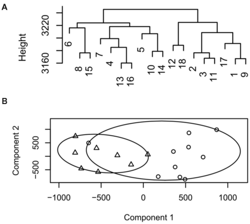
The agglomerative hierarchical clustering approach builds clusters by repeatedly joining and merging the objects separated by the shortest distance. Following merging of the closest two points the distance matrix is updated and the process repeated until all objects are joined. Commonly used non-hierarchical methods include k-means, k-medoids (also known as partitioning around medoids, PAM), and fuzzy clustering. In k-means/medoids the size of the resulting clusters (k) are defined a priori and n observations are then partitioned in k sets. k-means/medoids are agglomerative methods meaning that once a cluster has been formed it cannot be split and hence the points at which clusters are initialized needs to be randomized and repeated to ensure that stable final clusters are obtained. The advantages of this approach are simplicity and speed. Due to the initiation positions the disadvantage is that it does not yield the same result with each run, since the resulting clusters depend on the initial random assignments. For k-medoids the medoid is defined as the center point of the cluster in which the average dissimilarity is minimized for all objects of the cluster. The advantage of k-medoids over k-means is that random medoid points in the clusters are initialized and the closest medoids calculated. This is then repeated until all the medoids in the cluster remain stable. The result of hierarchical clustering is visualized as a dendrogram, whereas k-means/medoids analysis are plotted as clustergrams (Figure 1). In a dendrogram, “distance” is represented as the y axis. If the dataset is small enough to be visualized, a dendrogram is often preferable because “distance” conveys directly interpretable information. Collectively the above methods are referred to as “crisp” because they produce results where an element is placed in a single cluster or partition. In contrast to these, fuzzy clustering based on fuzzy logic can be applied. In this approach individual elements can belong to multiple clusters with different probabilities. The most widely used fuzzy clustering method is fuzzy C-means clustering (Bezdek, 1974).

Figure 1.

Example dendrogram and cluster plot from low decisive data. (A) Dendrogram, samples 1–9 represent group 1, 10–18 group 2. (B) Cluster plot output for the same data circles represent group 1, triangles group 2.

With this multitude combination of approaches and distance/linkage measures selecting the most appropriate to use is not at trivial task. In this manuscript we describe the comparison of these methods under different simulated methylation datasets. In this way we can determine the stability and reliability of methods for clustering of methylation beta-values.

Materials and Methods

Simulation of data

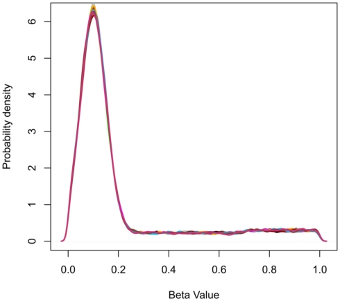
Data were simulated to represent the beta-values of illumina 27K arrays. To simulate a common preliminary data set, each data set contained 27,000 probes with 18 samples, which were divided into 2 groups of 9 samples. The distribution of beta-values on a 27K array does not follow a normal distribution but is biased with many probes showing low beta-values (due to hypomethylation of CpG islands; Figure 2). To compare the influence of the information content of simulated data sets the percentage of probes which separate each group (referred to as decisive probes) and the range of groups was varied. Fifteen simulated conditions were compared; five differences in percentage of decisive probes (0.1, 0.5, 1, 5, and 10% of total data) and three ranges of beta-values separating the two groups. For conditions of simulations see Tables 2 and 3.

Figure 2.

Probability density plots showing the frequency distribution of beta-values for simulated data. The peak at beta-value at approximately 0.1 represents the abundance of hypomethylated CpGs in CpG islands.

Table 2.

Parameters for simulation of data sets.

	Percentage of probes	Group 1 range	Group 2 range
Invariable (hypomethylated)	75%	Selected from normal distribution (mean 0.1 SD 0.05) lower bound = 0
Invariable (hypermethylated)	2%	0.7–1.0
Hyper variable	100-75-2-x	0–1.0
Decisive	x	See Table 3	See Table 3

Table 3.

Ranges of simulated values for each of 15 simulated data.

Simulation	Percent of decisive probes	Group 1 beta-values		Group 2 beta-values		Group differences
		Min	Max	Min	Max	Min	Max
S1	0.1	0.0	0.3	0.7	1.0	0.4	1.0
S2	0.1	0.3	0.5	0.6	0.7	0.1	0.4
S3	0.1	0.4	0.5	0.6	0.8	0.1	0.4
S4	0.5	0.0	0.3	0.7	1.0	0.4	1.0
S5	0.5	0.3	0.5	0.6	0.7	0.1	0.4
S6	0.5	0.4	0.5	0.6	0.8	0.1	0.4
S7	1.0	0.0	0.3	0.7	1.0	0.4	1.0
S8	1.0	0.3	0.5	0.6	0.7	0.1	0.4
S9	1.0	0.4	0.5	0.6	0.8	0.1	0.4
S10	5.0	0.0	0.3	0.7	1.0	0.4	1.0
S11	5.0	0.3	0.5	0.6	0.7	0.1	0.4
S12	5.0	0.4	0.5	0.6	0.8	0.1	0.4
S13	10.0	0.0	0.3	0.7	1.0	0.4	1.0
S14	10.0	0.3	0.5	0.6	0.7	0.1	0.4
S15	10.0	0.4	0.5	0.6	0.8	0.1	0.4

Cluster analysis

For each of the 15 simulation conditions 1000 replicate data sets were generated and clustering was conducted using k-medoids (using PAM of the cluster package), Fuzzy (using Fanny of the cluster package), and hierarchical clustering (using hclust). For PAM and Fanny the distance measures Euclidean, maximum, Manhattan (Larson and Sadiq, 1983), and Canberra (Lance and Williams, 1966) were used. These distance measures represent a standard set of distance measures commonly available however this list is not exhaustive, for additional measures (see Gower, 2005). For hclust the same distance measures were used in combination with Ward, single, complete, average, Mcquitty, median, and centroid linkage methods. The adjusted rand index (Rand, 1971) was used to determine clustering accuracy. The arandi method of the mcclust package was used to compare obtained cluster vectors to a cluster vector perfectly separating the two groups. In this way a rand index score of 1 represents perfect clustering with values less than 1 representing decreasing accuracy. Additionally the mean silhouette width of every member of a cluster group was determined to provide a measure of crispness of group separation (Rousseeuw, 1987). All R packages were obtained from the Comprehensive R Archive Network (CRAN http://cran.r-project.org/).

Results

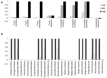
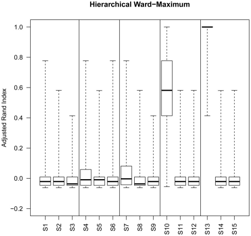
Although the range of separation of different groups in the simulations affects the outcome, i.e., simulations with groups separated by a larger amount (simulations 1, 4, 7, 10, and 13; see Table 3) are more likely to result in higher rand scores, the total number of decisive data points largely determines cluster accuracy. By grouping the simulations into three groups low (0.1 and 0.5% decisive data), mid (1% decisive data), and high (5 and 10% decisive data) this trend is consistent regardless of approach used (Figure 3). Comparison of the approaches does show some clear trends, in the low and mid range decisive data, fuzzy clustering performs poorly when using the rand index as a measure of accuracy. Likewise, the maximum distance measure does not perform well for the beta-value data when using any of the approaches or linkage methods. Within the hierarchical clustering approaches the centroid and median linkage methods also performed poorly. Of the hierarchical methods the Ward, Mcquitty, complete, and average linkage methods appear to be most robust producing the highest median rand score across simulations. Analysis of the mid and high decisive data ranges produce very consistent results. With the exceptions above, the median rand index approaches one for all methods when ≥1% decisive data is reached. Therefore the comparison of the low decisive data ranges may be more informative to determine the most appropriate method. Under these conditions the Ward–Manhattan method provides the most consistent results and generally outperforms other approaches. The Manhattan distance measure in combination with k-medoid, average, Mcquitty, complete, or Ward linkage methods produces the top five highest median rand index scores in the low decisive data category. The summary box plots of all simulations with all methods are given as Figure A1 in Appendix.

Figure 3.

The median rand index from 1000 simulations for all combinations of clustering, distance measure and linkage method used. (A) Fuzzy and k-medoids approaches, (B) hierarchical clustering approaches. For clarity the data was combined into three groups, low (0.1 and 0.5% decisive data), mid (1% decisive data), and high (5 and 10% decisive data).

The results of simulations suggest that the hierarchical Ward–Manhattan approach provides a consistent approach and that the Manhattan distance appears to be the best metric to separate clusters based on beta-values. However, this result is not absolute with some conditions particularly under low decisive data conditions resulting in inconsistency. As the hierarchical and non-hierarchical clustering approaches produce comparable results the choice between these methods largely comes to the visualization of output. As described in the introduction, for data sets with a limited number of samples we prefer the use of dendrograms for their ease of interpretation. Due to this the following section will focus on the comparison of hierarchical clustering methods.

The use of hierarchical clustering with novel biological data

From the comparisons above, the rand score is hugely useful in determining accurate clustering methods when analyzing simulated data, or for testing the output compared to a predicted or known “correct” clustering. However, when analyzing biological data without such a priori information how can we determine the “best” clustering approach when we cannot be sure of the amount of decisive data available?

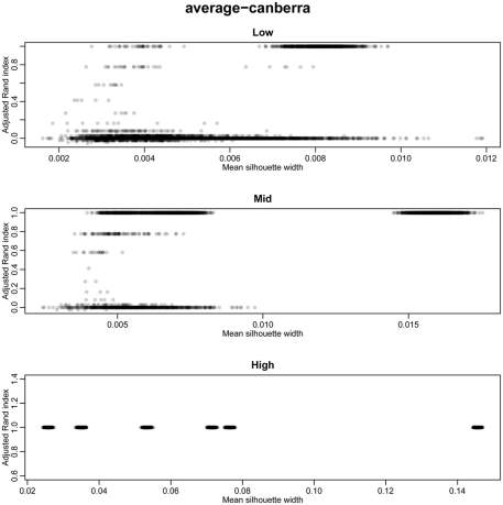
The silhouette width is a score used to determine the relatedness of samples in a cluster and the separation of different clusters (Rousseeuw, 1987). This provides a measure that can be used to determine the best clustering approach. However, can a cut-off of a good silhouette width be determined? Whilst it is clear that increased amounts of decisive data or better clustering approaches results in clearer clusters and greater silhouette widths, the average silhouette width and rand index do not correlate well (Figure 4). Analysis of the Ward–Manhattan method which produces consistent clustering highlights the variability of silhouette width even when a rank index of 1 is obtained. In this case the silhouette width ranges from approximately 0.05–0.4 (Figure 4A). Analysis of the Centroid–Euclidean method which is a less consistent method shows that the silhouette width varies when the clusters are poorly defined (low Rand index). Only when the clusters are correct (rand index = 1) does the silhouette width does settle to approximately 0.4 (Figure 4B). Results for all comparisons are given as a Figure A2 in Appendix.

Figure 4.

Scatter plots of rand index versus mean silhouette width. A gray scale of dots is used to show the density of clustering, black dots represent highest density. Low (0.1 and 0.5% decisive data), mid (1% decisive data), and high (5 and 10% decisive data). (A) Results obtained using the Ward linkage and Manhattan distance measures. (B) Results obtained using the centroid linkage and Euclidean distance measures.

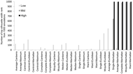
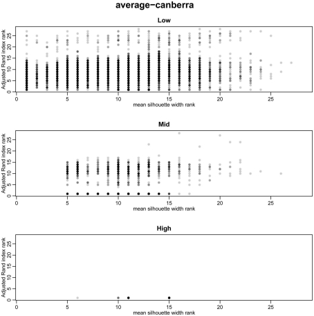
To overcome the lack of a defined cut-off of what constitutes an adequate silhouette width, we propose a consistent method is to rank the silhouette width to obtain the best clustering method. In this way we generate 28 clusterings for any given data set by combination of four distance measures with each of seven linkage methods and rank using the mean silhouette width. Thus the silhouette rank of one is the greatest silhouette width (equal scores are each given the lowest rank score). By comparing the median number of times in 1000 independent simulations each method achieves the top silhouette rank it is clear that certain methods again tend to produce more crisp clusters. As before the centroid and median linkage methods perform poorly. The Manhattan distance in combination with various linkage methods (single, average, complete, Mcquitty, and Ward) provides the most consistent results, i.e., is most often the highest ranked silhouette width when the percentage of decisive data is ≥1% (mid and high ranges in Figure 5). Whilst this shows that certain methods are always ranked highest does it follow that the highest ranked method produces the best results? By also ranking the outcome of the simulated data sets using the rand index and comparing the ranks of silhouette width and rand index we can show that methods with a high mean silhouette width produce more correct clustering. Scatter plots of the silhouette rank and rand index rank for all comparisons are given as Figure A3 in Appendix.

Figure 5.

The median number of highest silhouette rank obtained from 1000 simulations for each combination of distance measure and linkage method used. For clarity the data was combined into three groups, low (0.1 and 0.5% decisive data), mid (1% decisive data), and high (5 and 10% decisive data).

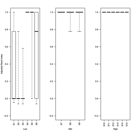
Analysis of the rand index scores obtained for the top ranked method (as determined using the greatest mean silhouette width) show that even at 0.5% decisive data points (simulations S4–S6) the top ranked silhouette width produces a median rand index of greater than 0.75 (Figure 6). For simulations with ≥1% decisive data points the median rand score is 1. Thus the approach to rank methods by silhouette width is a consistent approach for obtaining the best clustering results regardless of the method used to obtain the cluster. Software (Cluster Rank R code) used to compare and rank cluster methods are freely available from the authors or from http://www.nottingham.ac.uk/∼svzrde/software.htm.

Figure 6.

Box plots of adjusted Rand index for the top ranking method (as determined by silhouette width rank) for 1000 replicates of each simulation (S1–S15). For each figure the solid horizontal line represents the median rand index, the box contains the interquartile range and the whiskers mark the minimum and maximum values. For clarity the data was combined into three groups, low (0.1 and 0.5% decisive data), mid (1% decisive data), and high (5 and 10% decisive data).

Discussion

The visualization of the outcome of methylation can be either on a per gene or genome-wide basis. The latter allows an exploratory view of the data to be undertaken. Thus the use of methylation data is an expanding approach in the field of epigenomics and has been used for various studies (e.g., Banister et al., 2011; Cotton et al., 2011; Fackler et al., 2011; Fryer et al., 2011; Martino et al., 2011). Whilst the use of cluster methods have been widely used in many transcriptomics studies the use and limitations of these methods for analysis of methylation array data have not previously been determined. The simulations conducted here have shown a number of key findings. The first, that the amount of decisive data determines the ability to accurately separate groups is perhaps not surprising. The percentage of decisive data represents the signal within the background noise of hyper- and non-variable data. When the percentage of decisive data points is greater than 1% most methods can accurately capture the true clusters within the data. With the exception of the centroid and median linkage methods the hierarchical methods performed comparably. In contrast, the fuzzy methods required a larger percentage (5–10%) of decisive data to produce a comparable median rank index of 1. This is likely to reflect the nature of the fuzzy method where the strength rather than absolute membership of a sample to a group is determined. In this comparison we have used a crisp measure (Rand index) to determine the performance of a fuzzy method. Whilst the fuzzy C-means approach may not be directly of use for such exploratory investigations, this approach is of potential use as a measure to detect samples or biomarkers with a high variability between groups. The potential of this is being actively pursued. As described above the hierarchical and k-medoids methods produced similar results. Whilst the k-medoid approach has a slight advantage in speed, the choice of method is largely determined by output preference. In our experience the dendrogram output of the hierarchical method is more easily interpretable when the group sizes are not too large.

We propose a method to capture the best clustering outcome. As no one linkage and distance combination consistently outperformed others we suggest to use the silhouette width to rank the outcome of each algorithm. This produced a consistent improvement in cluster accuracy (as determined by rand index) than any one method alone. This approach has been successfully used to compare and analyze human clinical data (Emes et al., in preparation). Alternatives to this approach such as consensus clustering (also called ensemble clustering; Monti et al., 2003) which aims to find stable clustering solutions by validating multiple clustering outcomes from one or several applied algorithms may be complementary to our approach. However, our approach is relatively quick method even for large datasets of 450K arrays (results not shown). The simulation framework described here is deliberately a simplistic one where we are interested in the ability to differentiate into two clusters of equal size. Future research and refinement may look to simulate the effect of clustering groups of varying size and cluster number. However, the software developed can currently be used with any number of user defined clusters. In addition the software incorporates the implementation of the pvclust package (Suzuki and Shimodaira, 2006) which quantifies the uncertainty of each node in a hierarchical cluster. In this way probabilities are calculated using multiscale bootstrap resampling to determine to what extent each node is supported by the data. Using this approach the internal resolution of the clusters is also investigated. This approach therefore provides a robust framework for the investigation of data and for the identification of biomarkers or quality control of methylation samples in epigenomic studies.

Conflict of Interest Statement

The authors declare that the research was conducted in the absence of any commercial or financial relationships that could be construed as a potential conflict of interest.

Appendix

Figure A1.

Box plots of rand index scores across all simulations. For each figure the solid horizontal line represents the median rand index, the box contains the interquartile range and the whiskers mark the minimum and maximum values.

Figure A2.

Scatter plots of rand index versus mean silhouette width across all simulations. A gray scale of dots is used to show the density of clustering, black dots represent highest density. Low (0.1 and 0.5% decisive data), mid (1% decisive data), and high (5 and 10% decisive data).

Figure A3.

Scatter plots of rand index rank versus mean silhouette width rank across all simulations. A gray scale of dots is used to show the density of clustering, black dots represent highest density. Low (0.1 and 0.5% decisive data), mid (1% decisive data), and high (5 and 10% decisive data).

References

- Banister C. E., Koestler D. C., Maccani M. A., Padbury J. F., Houseman E. A., Marsit C. J. (2011). Infant growth restriction is associated with distinct patterns of DNA methylation in human placentas. Epigenetics 6, 920–927 10.4161/epi.6.7.16079 [DOI] [PMC free article] [PubMed] [Google Scholar]
- Bezdek J. C. (1974). Numerical taxonomy with fuzzy sets. J. Math. Biol. 1, 57–71 10.1007/BF02339490 [DOI] [Google Scholar]
- Bibikova M., Barnes B., Tsan C., Ho V., Klotzle B., Le J. M., Delano D., Zhang L., Schroth G. P., Gunderson K. L., Fan J. B., Shen R. (2011). High density DNA methylation array with single CpG site resolution. Genomics 98, 288–295 10.1016/j.ygeno.2011.07.007 [DOI] [PubMed] [Google Scholar]
- Bibikova M., Fan J. B. (2009). GoldenGate assay for DNA methylation profiling. Methods Mol. Biol. 507, 149–163 10.1007/978-1-59745-522-0_12 [DOI] [PubMed] [Google Scholar]
- Bibikova M., Fan J. B. (2010). Genome-wide DNA methylation profiling. Wiley Interdiscip. Rev. Syst. Biol. Med. 2, 210–223 [DOI] [PubMed] [Google Scholar]
- Cotton A. M., Lam L., Affleck J. G., Wilson I. M., Penaherrera M. S., Mcfadden D. E., Kobor M. S., Lam W. L., Robinson W. P., Brown C. J. (2011). Chromosome-wide DNA methylation analysis predicts human tissue-specific X inactivation. Hum. Genet. 130, 187–201 10.1007/s00439-011-1007-8 [DOI] [PMC free article] [PubMed] [Google Scholar]
- Du P., Zhang X., Huang C. C., Jafari N., Kibbe W. A., Hou L., Lin S. M. (2010). Comparison of beta-value and M-value methods for quantifying methylation levels by microarray analysis. BMC Bioinformatics 11, 587. 10.1186/1471-2105-11-587 [DOI] [PMC free article] [PubMed] [Google Scholar]
- Eads C. A., Danenberg K. D., Kawakami K., Saltz L. B., Blake C., Shibata D., Danenberg P. V., Laird P. W. (2000). MethyLight: a high-throughput assay to measure DNA methylation. Nucleic Acids Res. 28, E32. 10.1093/nar/28.8.e32 [DOI] [PMC free article] [PubMed] [Google Scholar]
- Everitt B. S., Landau S., Leese M., Stahl D. (2011). “Measurement of proximity,” in Cluster Analysis, eds Balding D. J., Cressie N. A. C., Fitzmaurice G. M., Goldstein H., Molenberghs G., Scott D. W., Smith A. F. M., Tsay R. S., Weisberg S. (Chichester: John Wiley and Sons, Ltd.), 43–69 [Google Scholar]
- Fackler M. J., Umbricht C. B., Williams D., Argani P., Cruz L. A., Merino V. F., Teo W. W., Zhang Z., Huang P., Visvananthan K., Marks J., Ethier S., Gray J. W., Wolff A. C., Cope L. M., Sukumar S. (2011). Genome-wide methylation analysis identifies genes specific to breast cancer hormone receptor status and risk of recurrence. Cancer Res. 71, 6195–6207 10.1158/0008-5472.CAN-11-1630 [DOI] [PMC free article] [PubMed] [Google Scholar]
- Fryer A. A., Emes R. D., Ismail K. M., Haworth K. E., Mein C., Carroll W. D., Farrell W. E. (2011). Quantitative, high-resolution epigenetic profiling of CpG loci identifies associations with cord blood plasma homocysteine and birth weight in humans. Epigenetics 6, 86–94 10.4161/epi.6.1.13392 [DOI] [PMC free article] [PubMed] [Google Scholar]
- Gower J. C. (2005). “Similarity, dissimilarity, and distance measure,” in Encyclopedia of Biostatistics, eds Armitage P., Colton T. (John Wiley and Sons, Ltd.). [Google Scholar]
- Houseman E. A., Christensen B. C., Yeh R. F., Marsit C. J., Karagas M. R., Wrensch M., Nelson H. H., Wiemels J., Zheng S., Wiencke J. K., Kelsey K. T. (2008). Model-based clustering of DNA methylation array data: a recursive-partitioning algorithm for high-dimensional data arising as a mixture of beta distributions. BMC Bioinformatics 9, 365. 10.1186/1471-2105-9-365 [DOI] [PMC free article] [PubMed] [Google Scholar]
- Irizarry R. A., Ladd-Acosta C., Wen B., Wu Z., Montano C., Onyango P., Cui H., Gabo K., Rongione M., Webster M., Ji H., Potash J. B., Sabunciyan S., Feinberg A. P. (2009). The human colon cancer methylome shows similar hypo- and hypermethylation at conserved tissue-specific CpG island shores. Nat. Genet. 41, 178–186 10.1038/ng.298 [DOI] [PMC free article] [PubMed] [Google Scholar]
- Kuan P. F., Wang S., Zhou X., Chu H. (2010). A statistical framework for illumina DNA methylation arrays. Bioinformatics 26, 2849–2855 10.1093/bioinformatics/btq553 [DOI] [PMC free article] [PubMed] [Google Scholar]
- Lance G. N., Williams W. T. (1966). Computer programs for hierarchical polythetic classification (similarity analyses). Comput. J. 9, 60–64 [Google Scholar]
- Larson R. C., Sadiq G. (1983). Facility locations with the Manhattan metric in the presence of barriers to travel. Oper. Res. 31, 652–669 10.1287/opre.31.4.652 [DOI] [Google Scholar]
- Marjoram P., Chang J., Laird P. W., Siegmund K. D. (2006). Cluster analysis for DNA methylation profiles having a detection threshold. BMC Bioinformatics 7, 361. 10.1186/1471-2105-7-361 [DOI] [PMC free article] [PubMed] [Google Scholar]
- Martino D. J., Tulic M. K., Gordon L., Hodder M., Richman T., Metcalfe J., Prescott S. L., Saffery R. (2011). Evidence for age-related and individual-specific changes in DNA methylation profile of mononuclear cells during early immune development in humans. Epigenetics 6, 1085–1094 10.4161/epi.6.9.16401 [DOI] [PubMed] [Google Scholar]
- Monti S., Tamayo P., Mesirov J., Golub T. (2003). Consensus clustering: a resampling-based method for class discovery and visualization of gene expression microarray data. Mach. Learn. 52, 91–118 10.1023/A:1023949509487 [DOI] [Google Scholar]
- Rand W. M. (1971). Objective criteria for the evaluation of clustering methods. J. Am. Stat. Assoc. 66, 846–850 10.2307/2284239 [DOI] [Google Scholar]
- Rousseeuw P. J. (1987). Silhouettes – a graphical aid to the interpretation and validation of cluster-analysis. J. Comput. Appl. Math. 20, 53–65 10.1016/0377-0427(87)90125-7 [DOI] [Google Scholar]
- Schmutte C., Fishel R. (1999). Genomic instability: first step to carcinogenesis. Anticancer Res. 19, 4665–4696 [PubMed] [Google Scholar]
- Siegmund K. D., Laird P. W., Laird-Offringa I. A. (2004). A comparison of cluster analysis methods using DNA methylation data. Bioinformatics 20, 1896–1904 10.1093/bioinformatics/bth176 [DOI] [PubMed] [Google Scholar]
- Steemers F. J., Chang W., Lee G., Barker D. L., Shen R., Gunderson K. L. (2006). Whole-genome genotyping with the single-base extension assay. Nat. Methods 3, 31–33 10.1038/nmeth842 [DOI] [PubMed] [Google Scholar]
- Suzuki R., Shimodaira H. (2006). Pvclust: an R package for assessing the uncertainty in hierarchical clustering. Bioinformatics 22, 1540–1542 10.1093/bioinformatics/btl117 [DOI] [PubMed] [Google Scholar]