Interaction mining and skill-dependent recommendations for multi-objective team composition

Abstract

Web-based collaboration and virtual environments supported by various Web 2.0 concepts enable the application of numerous monitoring, mining and analysis tools to study human interactions and team formation processes. The composition of an effective team requires a balance between adequate skill fulfillment and sufficient team connectivity. The underlying interaction structure reflects social behavior and relations of individuals and determines to a large degree how well people can be expected to collaborate. In this paper we address an extended team formation problem that does not only require direct interactions to determine team connectivity but additionally uses implicit recommendations of collaboration partners to support even sparsely connected networks. We provide two heuristics based on Genetic Algorithms and Simulated Annealing for discovering efficient team configurations that yield the best trade-off between skill coverage and team connectivity. Our self-adjusting mechanism aims to discover the best combination of direct interactions and recommendations when deriving connectivity. We evaluate our approach based on multiple configurations of a simulated collaboration network that features close resemblance to real world expert networks. We demonstrate that our algorithm successfully identifies efficient team configurations even when removing up to 40% of experts from various social network configurations.

1. Introduction

Over the last years, we have observed a trend towards crowdsourcing of knowledge intensive tasks. This novel model for problem solving received not only attention from academia but also global marketplayers. Currently crowdsourcing is mostly applied in cases where a larger task is segmented into many small work items that are carried out by individual knowledge workers. Usually there is no interaction between those workers. We expect that the tasks carried out in the crowd will become more complex, thereby requiring the complementary skills from multiple experts. Unlike traditional team-based work, however, members of the crowd are distributed and in many cases without those obligations as found in companies (long-term contracts or roles) [1]. The crowd presents a pool of experts, who are connected amongst themselves forming a social network. Relations between experts in this scenario typically emerge based on previous interactions in context of collaborative tasks. These links are weighted to describe the frequency of previous interactions. The crowd is self-managing as members are free to join or leave at any time. In this setting, team composition describes the short-term formation of a set of experts that provide the required skills.

Simply trying to find the smallest group of experts exhibiting all required skills is no longer a valid approach. A major factor of team success, for instance, is whether a set of experts can work together effectively [2,3]. The frequency of previous interactions is one possible indicator of successful collaborations. Crowds dynamics, however, exhibit a major challenge. The likelihood of finding a strongly connected expert team, providing the exact set of skills is low as experts dynamically take up work assignments and thus are not always available. For team compositions we consider the following aspects: (i) Skills describe the desirable properties an expert offers to complete a task. For each skill, a quality metric describes the expert's experience. The primary objective in workforce allocation is to find the team with the best coverage of the required skills. (ii) Interaction Distance is an indicator of how well users work together. Previous interactions form a weighted social network. Ideally, every member of a team has already worked with every other team member before. We assume that strong relations reflect multiple, successfully completed collaborative tasks. (iii) Load determines the short-term availability of users. Experts that are not available cannot become part of a new team. Instead of eliminating them from the candidate set, we let them act as referees by applying their social network for recommending other experts of their respective fields. However, with growing number of experts and skills, as well as inherent dynamics in large-scale networks, discovering efficient team compositions that fulfill multiple criteria becomes a complex problem. In order to address this NP complete challenge novel heuristics are required.

Our salient contributions in this paper are:

• • Team Composition Discovery Heuristic. We introduce the application of genetic algorithms and simulated annealing for determining effective workforces which provide sufficient skill coverage while achieving adequate team connectivity. Such team configurations promise higher probability of success in future collaborations compared to team configurations that neglect social relations and account for individual skills only.
• • Skill-dependent Recommendation Model. We highlight an innovative skill-dependent, team-centric recommendation model where recommendations are driven by the interaction structure of the current team members, thus customized for a given situation, and not based on a global reputation metric only.
• • Self-Adjusting Trade-Off Model. We apply self-adjusting mechanisms that determine the trade-off between interaction distance and recommendations in order to unburden users from tedious configuration tasks and manual management of team compositions.

Our main findings show that a dynamic balance of interactions and recommendations provides better team configurations than relying on one strategy alone. Thus our approach can always provide a better trade-off between skill coverage and team connectivity, regardless of the percentage of unavailable experts.

The remainder of this paper is organized as follows. Related work in Section 2 compares the novelty of our approach to existing research efforts. The motivating scenario in Section 3 outlines the combination of direct interactions and recommendations and provides an overview of our approach. Section 4 outlines the problem in more detail and provides an approach outline. Section 5 explains the skill-based recommendation model. Section 6 discusses the details on the team allocation algorithm. In Section 7 we analyze the performance of our algorithm based on data from our expert network formation model which replicates the key characteristics of real world expert networks. Finally, we provide an outlook on future work and conclusion of the paper in Section 8.

2. Related work

Team formation is an intensely studied problem in the operation research domain. Most approaches model the problem as finding the best match of experts to required skills taking into account multiple dimensions from technical skills, cognitive properties, and personal motivation [2–4]. Such research focuses only on properties of individual experts that are independent of the resulting team configuration.

Recent efforts introduce social network information to enhance the skill profile of individual members. Hyeongon et al. [3] measure the familarity between experts to derive a person's know-who. Cheatham and Cleereman [5] apply social network analysis to detect common interests and collaborations. The extracted information, however, is again applied independently from the overall team structure. These mechanisms present opportunities for refinement of the skill modeling and configuration aspects of our approach but remain otherwise complementary.

Multiple efforts address related group formation problems. Sozio and Gionis describe the community formation problem [6]. Given a set of fixed members, the approach expands the team up to a maximum upper size boundary such that the communication cost within the community remains small. Anagnostopoulos et al. [7] address fair task distribution within a team. They apply skill matching to determine a team's ability to fulfill the overall set of tasks. While their approach takes into account team members' load and skill dependencies, the underlying social network structure has no impact on the team's fitness. Yang et al. [8] apply integer programming to determine the best set of group members available at a certain point in time. Their temporal scheduling technique considers the social distance between group members to avoid lacking too many direct links. Craig et al. [9] propose an algorithm for reasonably optimal distribution of students into groups according to group and student attributes. Xie et al. [10] aggregate a set of recommender results to optimally compose a package of items given some relation between the individual items and an overall package property (e.g., holiday package). Datta et al. [11] showcase a demo for skill-based, cohesion-aware team formation that utilizes common citations for establishing a social network. The authors, however, remain silent on specific details about the actual algorithm to find an optimal team. An alternative approach is first finding tightly connected communities [12] and then analyzing the available skills to generate desirable team configurations.

To the best of our knowledge, Theodoros et al. [13] discuss the only team composition approach that specifically focuses on the expert network for determining the most suitable team. Our approach differs in three significant aspects. First, we model a trade-off between skill coverage and team connectivity whereas [13] treats every expert above a certain skill threshold as equally suitable and ignores every expert below that threshold. Second, our algorithm aims for a fully connected team graph (i.e., relations between every pair of experts). Theodoros et al. optimize the team connectivity based on a minimum spanning tree (MST). We argue that it is more important to focus on having most members well connected (i.e. everybody trusts (almost) everybody else) within the team than focusing on having each member tightly connected to only one other member. Also Singh [14] shows that a densely connected team is vital for successful open source developer cooperation. Most importantly we apply recommendations instead of direct interaction links when the underlying network becomes too sparsely connected.

Analysis of various network topologies [15,16] has demonstrated the impact of the network structure on efficient team composition. General research on the formation of groups in large scale social networks [17] helps to understand the involved dynamic aspects but does not provide the algorithms for identifying optimal team configurations. Investigations into the structure of various real-world networks provides vital understanding of the underlying network characteristics relevant to the team composition problem [18,19]. Papers on existing online expert communities such as Slashdot [20] and Yahoo! answers [21] yield specific knowledge about the social network structure and expertise distribution that need to be supported by a team composition mechanism.

Complementary approaches regarding extraction of expert networks and their skill profile include mining of email data sets [22,23] or open source software repositories [24]. Additional sources include (scientific) publications and financial data [25], social network page visits [26], telecommunication data [27], and online forum posts [28].

Related research efforts based on non-functional aspects (i.e., non-skill related aspects) can also be found in the domain of service composition [29]. Here, services with the required capabilities need to be combined to provide a desirable, overall functionality. Composition is driven by the client's preferences [30], environment context [31,32], or service context (i.e., current expert context) [33]. We can take inspiration from such research to refine the properties and requirements of teams to include context such as expert's organization or location. Nonetheless, the network structure remains equally unexplored in service composition.

In contrast, the network structure has gained significant impact for determining the most important network element. A prominent example of a graph-based global importance metric is Google's page rank [34]. An extended version [35] yields total ranks by aggregating search-topic-specific ranks. Balog and De Rijke [36] extract a social profile from collaborations within intranets to find suitable experts. The Aardvark search engine by Horowitz and Kamvar [37] leverages social ties for expert finding in a user's extended network. Inspired by the page rank algorithm, Schall [38] applies interaction intensities and skills to rank humans in mixed service-oriented environments. These algorithms and frameworks provide additional means to determine person-centric metrics but do not address the team composition problem per se. The potential of expert finding applications, however, and subsequently the impact on team formation cannot be underestimated. Social network-based expert finding and subsequently team formation will soon become central business concerns [39].

The model of recommendation-based link establishment is closely related to link prediction in social networks. Such models are used to introduce connections between single members of a community by evaluating various properties. For instance, work by [40,41] discusses link prediction based on similarity, focusing on structural graph properties such as number of neighbors and number of in/out links.

In social trust networks [42] recommendations reflect transitive relations among members. In that case, unconnected nodes in a trust network are connected through an intermediate node that mediates second hand knowledge among its neighbors. In the future, direct trust between humans will play an ever more important role as privacy remains a largely unsolved challenge [43]. Hence we believe that establishing explicit trust in social networks (e.g., [44,45]), respectively becoming aware of distrust, will become a significant factor in team formation.

3. Motivational scenarios and fundamental issues

In today's highly dynamic large-scale networks, people are no longer able to keep track of the dynamics, such as registration of new actors in expert networks and emerging skills and expertise of collaboration partners. Since interactions and collaborations on the Web are observable, systems can analyze tasks performed in the past in order to determine network structures and member profiles automatically [46,42]. Based on these assumptions, our work aims at discovering effective member compositions, i.e., teams, in collaborative network for given tasks that demand for particular skills. For that purpose we do not only consider skills and expertise of single members but also their social embedding in their respective communities.

3.1. Application scenarios

Here we demonstrate the wide applicability of our approach in a large area of motivating use case scenarios:

• • Crowdsourcing. Suppose that an IT consulting company outsources work to a crowd where a set of experts processes assigned tasks on demand. The incentive for processing tasks can be based on monetary rewards or other community based reputation schemes. However, the allocation of experts depends on people's skills and expertise. Especially complex tasks demand for compositions of experts having a wide variety of skills and expertise. In that case, also social structures need to be taken into account, for instance, to ensure compatibility of collaboration behavior and working styles.
• • Open Web-based Collaboration. A typical example for open Web-based collaboration is Wikipedia.¹ Here, people can freely interact with others to discuss issues of articles and potential improvement in order to increase overall quality. Groups of authors who frequently co-edit articles deem to be more efficient than totally unrelated authors. The reason is that authors already know each other's quality standards and detailed capabilities to share work efficiently.
• • Cross-Organizational Processes. Establishing cross-organizational social networks that span thousands of people across different departments and even organizational boundaries has been in a research focus since years. With the recent availability of fast and reliable communication networks these large-scale systems are being realized. A major focus of research in this area is to link geographically distributed people to build virtual teams assigned to global processes. One indicator for efficient team collaboration is the amount and density of interactions among its members. Once a team successfully performed a set of tasks, this composition should be encouraged and maintained to be reused for future work.

3.2. Problem outline

Increasing complexity of tasks demands for the assembly of multiple people to teams. This team assembly process is based on numerous constraints, including the set of demanded skills which a candidate group of workers needs to cover. In the following (Fig. 1 ), we outline inherent problems in detail and discuss various concepts and techniques that assist the composition of workforces.

Fig. 1.

Expert crowd interaction network (full lines) and recommendations (dotted lines). Line thickness represents the experts' distance based on weighted interactions, red/shaded nodes depict unavailable experts.

Fig. 1a shows an interaction (collaboration) network comprising members (nodes) and interaction links (edges). Each edge is associated with a weight depending on performed interactions (depicted by the line thickness). Let us consider 9 members of this network whose profiles match at least one required skill.² In particular, the skills of each node are given as A {p2p}, B {p2p}, C {ml, p2p}, D {we}, E {we, dm}, F{ml}, G {ml}, H {dm}, and J {dm, ml}. An optimal composition in this case can be established based on skill matching and weighted links between nodes. Thus, the optimal composition in this scenario is given by combining the capabilities of nodes B, C, and E.

Especially in large-scale and highly dynamic environments, however, the availability of people frequently changes and greatly influences the ability to utilize the skills of certain network members. Availability of people must be considered when composing a workforce. Suppose that C, H, and J are not available (see also red colored nodes in Fig. 1b) in this given setting. As C is not available, another candidate team solution comprising all required skills is the set {A,D, E, G}. The connectivity of this team is, however, rather low. The metric interaction distance is an indicator for the structural connectivity in collaboration networks. One of the novel contributions in this work is to use recommendations to identify suitable experts for replacing unavailable members. As shown in Fig. 1b, a match yielding tighter relations (based on interaction weights) can be obtained when considering {B, E, F}. Recommendations are based on skills (e.g., {ml} associated with the profiles of, for example, C and F), thereby introducing new links between nodes. For simplicity, we augment the visualization of the interaction network by showing these links as dashed lines. Recommendations help establish new collaborations between members of a network. In Fig. 1b, C recommends F to B, which subsequently results in forming a new link from B to F. The strength (weight) of the recommendation depends on the interaction-based distance of B and C as well as C and F.

While finding a suitable team in the given example is rather simple, the team formation problem becomes much more challenging in a large social network. With a linear increase in experts, the number of combinations to check grows exponentially. At the same time, the best connected experts – which are usually also the best skilled ones – display an increasing number of relations. Consequently, checking for recommendations becomes computationally expensive.

3.3. Approach outline

Three major stages describe the progress toward team composition:

• 1. Network Establishment. First, we establish a group of experts and corresponding social network (Fig. 2a) that provides the weighted interaction links among them, the respective skill profiles, and information about expert availability.
• 2. Candidate Selection. From this network, we select the set of team candidates which need to be available and provide at least one required skill (Fig. 2b). However, the top ranked experts provide the highest expertise but usually come with low connectivity.
• 3. Heuristic Optimization. Finally, team composition aims to find a better connected team based on direct interactions and recommendations while maintaining high skill coverage (Fig. 2c).

Fig. 2.

Lines represent weighted edges based on previous interactions; unavailable experts are marked in red (a). Dashed circles are the top experts for each skill amongst the team candidates (bordered area). The final expert configuration (black, filled circles) provides the best combination of skills and distance (c). Colors online.

4. Multi-objective team composition

4.1. Preliminaries

A team composition consists of experts, a weighted social network structure, and a set of skills $\mathcal{S}$. The social network is modeled as an undirected, weighted graph $\mathcal{G}$ _SN($\mathcal{U}$, $\mathcal{E}$) where the vertices are experts u  ∈  $\mathcal{U}$, and the edges represent collaborations in joint activities. The edge weight w _e describes the distance between two experts. A small edge weight represents frequent collaboration between two experts while a high edge weight describes rare collaboration. The proximity (Eq. (1)) of an expert to itself is zero (prox(u _i, u _i) = 0). The proximity prox(u _i, u _j) between two experts is defined by the shortest hop path (SHP) with minimum edge weights. We sum across all traversed edges and take the hop count (h) to account for the number of intermediary experts.

$$prox(u_i,u_j)=(h*(h-1)+1)*\sum _k{w}_h\forall w_h\in max\left[SHP\right(u_i,u_j\left)\right]\text{.}$$ (1)

An expert's skill profile $\mathcal{P}$ _i contains for each skill a corresponding expertise level q _i(s). The expertise level is measured on a scale from 0 to 1, where 1 describes the maximum achievable expertise. Set of required skills for a team is denoted as $\mathcal{S}$ _R  ⊆  $\mathcal{S}$. A valid team configuration $\mathcal{T}$($\mathcal{U}$ _T, $\mathcal{S}$ _R) consists of experts $\mathcal{U}$ _T  ⊆  $\mathcal{U}$, such that for each s _i  ∈  $\mathcal{S}$ _R there exists at least one expert u _j  ∈  $\mathcal{U}$ $\mathcal{T}$ providing that skill (q _j(s _i) >  q(s)_min with q(s)_min  ≥ 0). We identify the expert u assigned to provide skill s within team $\mathcal{T}$ as u $\mathcal{T}$(s).

We establish the collaboration network and skill profile through observation of user interactions. Each interaction takes place in the scope of an activity which in turn is associated with exactly one skill. The sum of all involvements in activities produces the expert's skill profile. Specifically for each skill, there exists a mapping function f _s($\mathcal{E}$ _u  ↦  q _u(s)) that determines the expertise level from the set of an expert's edges $\mathcal{E}$ _u.

Fig. 3 (top left) displays an excerpt from the interaction log of users Alice, Bob, Carol, and Dave.³ Alice and Bob have interacted together three times in a p2p related activity and once in a dm related activity. In total, Bob applied his p2p skills 6 times, his dm skills once, and his ml skill also only once. In this example, the mapping function f from edges to expertise level is a linear transformation. For each skill, we take the maximum skill occurrence (e.g., p2p  = 6), thus deriving Alice's expertise level of q _Alice(p2p) = 0.5.

Fig. 3.

Deriving skill profiles and weighted social network from interaction logs.

In addition to the skill profile, each expert provides load information to indicate his ability to participate in a new team. Load is modeled as a boolean value l _u  =  true  |  false where true denotes an available expert, while false denotes an overloaded expert.

4.2. Problem definition

Given a set of experts $\mathcal{U}$, a social network $\mathcal{G}$ _SN, and required skill set $\mathcal{S}$ _R, find the team configuration $\mathcal{T}$ that provides the best match of user skills to required skills while reducing team distance as much as possible. Having a multi-objective function, we aim at maximizing the skill coverage function $\mathcal{C}$ $\mathcal{T}$, while minimizing the team density function $\mathcal{D}$ $\mathcal{T}$. Additionally we need to satisfy the following constraints: for each skill there exists a lower threshold q(s)_min that defines the minimum expertise level within the team, and a set of team configuration constraints $\mathcal{G}$. Example constraints restrict the maximal number of skills a single expert may provide, or the minimum size of a team. How such constraints are formulated in detail is irrelevant at this point. Formally we can describe the team formation problem as follows:

$$\begin{array}{l}\text{maximize}\mathcal{C}\left(\mathcal{T}\right)\\ \text{minimize}\mathcal{D}\left(\mathcal{T}\right)\end{array}$$

such that:

$$\begin{array}{l}{u}_{\mathcal{T}}\left(s\right)>q{\left(s\right)}_{\mathit{min}}\forall s\in {\mathcal{S}}_R\\ g\left(\mathcal{T}\right)=\text{true}\forall g\in \mathcal{G}\text{.}\end{array}$$

Brute-force testing of every possible combination quickly becomes unfeasible. Testing m experts for $\left|{\mathcal{S}}_{\mathcal{R}}\right|$ skills has $\mathcal{O}$ $\left(m^{\left|{\mathcal{S}}_{\mathcal{R}}\right|}\right)$ computational complexity (i.e., already for 10 experts and 10 skills, we would need to analyze 10 billion combinations). In the next subsection, we show that the described team formation problem is NP-complete and thus requires a heuristic to derive good solutions. We further analyze the computational complexity for calculating a team's quality when discussing the heuristics in Section 6.7.

4.3. NP completeness

We demonstrate that the multi-objective team formation problem is NP complete by reducing it first to a single objective problem. We assume that for a particular skill s all experts with an expertise level above a certain threshold are equally well suited (q(s) >  req(s)). Thus, the problem is reduced to finding the team structure with the strongest ties in-between all members.

This problem is related to determining a clique in a weighted graph. At this moment, however, it is unclear which and how many experts are part of the best team. Also it is unlikely that this team actually exhibits a fully connected subgraph. Consequently we cannot directly search for the best clique yet. We model skills and interaction structure as a weighted complete k-partite graph. A k-partite graph consists of k distinct sets of nodes so that there are no edges between any two nodes in the same set. Edges exist between nodes of different sets. In a complete k-partite graph, every node is connected to (i.e., is adjacent to) every other node outside its set. For our problem, the set of required skills corresponds to the k sets in the k-partite graph. The nodes within each set are 2-tuples of expert and skill <  u, s>. An expert providing multiple skills above the threshold produces a tuple in each corresponding set. Ultimately, each set in the k-partite graph consists of tuples that contain the same skill s and all experts providing that skill. The edge weights between two tuples in different sets are given by the proximity measurement (see above) between the two corresponding experts.

Ultimately, a selection of exactly one tuple from each set constitutes a valid team where each tuple is connected to every other tuple in the team. The edges between the tuples determine the team's density. The tuples in the selection determine which experts are to provide what skill. When flattening the k-partite graph into a regular graph following properties hold: (i) any valid team will be a clique and (ii) the maximum clique size is k. The best team is then a matter of finding the minimum-weighted clique. This is trivially transformed into a maximum clique problem by inverting the edge weights. It is generally known that the maximum clique problem is NP-complete. We, thus, can infer that also the observed team formation problem is NP-complete.

4.4. Modeling the objective functions

To obtain a team's skill coverage $\mathcal{C}\left(\mathcal{T}\right)$ (Eq. (2)), we take the experience level of each expert assigned to provide a particular skill s within team $\mathcal{T}$. Ignoring any team constraints, the best possible composition consists of the best skilled experts (i.e., an expert having maximum experience level q(s) = 1) for every skill s  ∈  ${\mathcal{S}}_{\mathcal{R}}$. One user potentially covers multiple skills.

$$\mathcal{C}\left(\mathcal{T}\right)=\frac{{\sum }_{{\mathcal{S}}_{\mathcal{R}}}{u}_{\mathcal{T}}\left(s\right)}{\left|{\mathcal{S}}_{\mathcal{R}}\right|}whereu\in \mathcal{T}\forall s\in {\mathcal{S}}_{\mathcal{R}}\text{.}$$ (2)

We denote the best possible composition ($\mathcal{C}$($\mathcal{T}$) = 1) as Top(${\mathcal{S}}_{\mathcal{R}}$). This top expert composition, however, usually does not yield tight relations between the experts. Hence, we try to reduce a team's distance $\mathcal{D}$($\mathcal{T}$).

The distance function reflects our assumption that a-priori acquaintance of any two team members is crucial to successful collaboration. The direct team distance (Eq. (3)) is thus defined as the sum of link weights between members plus a penalty distance for non-existing links. The number of non-existing links are determined by calculate the maximum possible number of links between members, and subtracting the number of existing intra team links (|$\mathcal{E}$ _t|).

$${\mathcal{W}}_e\left(\mathcal{T}\right)=\sum _{\mathcal{T}}{w}_e(u_i,u_j)+\left(\left|\mathcal{T}\right|*(\left|\mathcal{T}\right|-1)*0.5-\left|{\mathcal{E}}_t\right|\right)*\beta *max\left(w_e\right)\forall u_i,u_j\in \mathcal{T}\text{.}$$ (3)

The penalty parameter β determines the impact on distance when we drop an edge with maximum weight max(w _e). For β  = 1, we treat two experts yielding link of max(w _e) as if they were not connected at all. If we set β too low, non-existing links are not penalized and we will not be able to find a better connected team than Top(${\mathcal{S}}_{\mathcal{R}}$). If we set β too high, only fully connected teams will yield low distance and thus be considered. A sensible value derived from our experiments is β  = 4 which we will use throughout this paper.

We inverse the distance objective function and instead of minimizing distance we aim to maximize the distance improvement (Eq. (4)) compared to the Top Team.

$$\mathcal{D}\left(\mathcal{T}\right)=\frac{{\mathcal{W}}_e\left(\mathcal{T}\right)}{W_e\left(Top\right({\mathcal{S}}_{\mathcal{R}}\left)\right)}$$ (4)

where W _e(Top(${\mathcal{S}}_{\mathcal{R}}$)) is the team distance of the Top Team.

We aggregated the objective functions in order to determine the best team. The overall composition quality $\mathcal{Q}$($\mathcal{T}$) (Eq. (5)) is given as a linear combination of skill coverage and distance improvement. The trade-off parameter α encodes a preference towards best coverage (α  ⊣ 1) or towards minimum distance (α  ⊣ 0).⁴ The optimum team configuration is then given by the composition with maximum quality.

$$Q\left(\mathcal{T}\right)=\alpha *\mathcal{C}\left(\mathcal{T}\right)+(1-\alpha )*\left(1-\mathcal{D}\left(\mathcal{T}\right)\right)with\alpha =[0,1]\text{.}$$ (5)

For a required skill set ${\mathcal{S}}_{\mathcal{R}}$  = {p2p, ml} and α  = 0.5, the best workforce of experts in Fig. 3 comprises users Alice and Bob. For $\mathcal{T}$ _A,B  = {Alice, Bob}, the skill coverage is $\mathcal{C}$(A, B) = 0.93, the distance amounts to $\mathcal{W}$ _e(A, B) = 0.50 (already applying the multi-skill per expert aware distance function as outlined in the next subsection). The overall quality yields $Q$(A, B) = 0.72. There is an alternative set $\mathcal{T}$ _B,D  = {Bob, Dave} that exhibits better coverage $\mathcal{C}$(B, D) = 1 but higher distance ($\mathcal{W}$ _e(B, D) = 0.5), which overall yields only $Q$(B, D) = 0.5.

4.5. Multiple skill provisioning

So far we have assumed that each expert in a composition provides exactly one skill. In some situations, it is beneficial to have an expert provide multiple skills. For a set of required skills ${\mathcal{S}}_{\mathcal{R}}$  = {p2p, ml, dm}, Bob can provide p2p and dm skills, while Alice provides ml. We need to create a new composition view to correctly calculate recommendations and ultimately also distance. We simply split an expert profile that provides multiple skills and create a virtual profile for every skill. In Fig. 4 , Bob's profile is separated into Bob1 and Bob2, one for p2p and dm respectively. Bob's social network edge set is replicated for each virtual profile.

Fig. 4.

Splitting an expert profile for Bob who provides multiple skills to correctly calculate recommendations and distance. Edges labels display the interaction weights (w_e). The weight of the interaction edge (red/double line) connecting profiles Bob1 and Bob2 obtains the minimum possible interaction edge weight (w_e = 0).

Distance needs to reflect the fact that an expert potentially provides multiple skills. So far teams with experts that provide multiple skills would yield lower distance. For the above listed example skill set ${\mathcal{S}}_{\mathcal{R}}$ we have three composition candidates: $\mathcal{T}$ _B1,D,A  = {Bob1, Dave, Alice} happens to be the Top team, $\mathcal{T}$ _B1,D,B2  = {Bob1, Dave, Bob2}, and $\mathcal{T}$ _B1,A,B2  = {Bob1, Alice, Bob2}. Table 1 left part provides the coverage, interaction distance, and overall quality for the multi-skill unaware distance calculation. Apparently, a composition of Alice and Bob is preferable over a composition comprising Alice, Bob, and Dave; which in turn outperforms a combination of Bob and Dave. When we compare $\mathcal{T}$ _B1,D,A and $\mathcal{T}$ _B1,D,B2 more closely, we notice that both provide the same skill coverage. $\mathcal{T}$ _B1,D,B2 , however, yields a better distance ratio as the distance measurement is unaware that Bob provides two skills.

Table 1.

Effect of multi-skill aware distance calculation on overall team composition quality.

	C($\mathcal{T}$)	We($\mathcal{T}$)	$Q$($\mathcal{T}$)	Wev($\mathcal{T}$)	$Q$v($\mathcal{T}$)
Top(${\mathcal{S}}_{\mathcal{R}}$) = TB1,D,A	1.00	1.00	0.50	1.00	0.50
TB1,D,B2	1.00	0.50	0.75	1.00	0.50
TB1,A,B2	0.93	0.25	0.82	0.50	0.72

The distance is more accurately represented when the distance calculation is based on the network including the virtual experts. This requires introducing an interaction link between the virtual expert profiles. In Fig. 4 the additional edge is displayed as a red, double line. As we assume that provisioning of two skills by the same expert does not raise any expert internal conflicts we apply the minimum possible interaction edge weight w _e(u _i, u _i) = 0.

Applying this new distance calculation we determine new distance measurements. The superscript v is used only in this section to distinguish between calculation with and without virtual profiles. Later calculations are virtual profile aware by default. The right part of Table 1 provides the multi-skill aware distance and quality measurements. We still observe $\mathcal{T}$ _B1,A,B2 as the best composition, however, $\mathcal{T}$ _B1,D,B2 is now considered of equal quality as $\mathcal{T}$ _B1,D,A as its distance is the same. Note that the distance calculation does not include recommendations yet. We outline in the following section how to integrate interaction weights and recommendations.

5. Expert recommendation

The goal of recommendation is to increase skill coverage and/or density by considering experts that are not directly connected to the existing team composition of experts $\mathcal{T}$. When Alice has frequently worked with Bob, and Bob in turn has frequently interacted with Carol, then Carol might be a suitable candidate in a composition with Alice when Bob is not available. Adding a non-connected expert to a composition, however, will greatly increase the team distance. In this section, we discuss how to use recommendations in the distance calculation to mitigate the effect of missing links.

Recommendations are skill dependent. For a given single recommendation in Fig. 5 between Alice and Carol (the recommendees) via Bob (the recommender), we observe which skills the two (disconnected) experts provide within the team. Here, Alice contributes skill dm while Carol is contributing skill p2p — Bob's particular role in the composition is irrelevant in this recommendation. The recommendation reflects then how well Bob can evaluate the expertise of both recommendees.

Fig. 5.

Single, skill dependent recommendation via expert Bob. Alice provides skill dm, while Carol provides skill p2p.

The recommendation's strength depends on two factors. First, both the expertise level of recommending expert and the expertise level of the recommended experts have impact. Two experts can increasingly well evaluate each other the higher their corresponding expertise levels are. Thus, the recommendation strength will be equal for a low-skilled expert recommending a high-skilled expert or whether the recommendation occurs in the opposite direction. In the former case, one cannot expect the low-skilled expert to give an accurate recommendation, while in the latter case the high-skilled expert will not fully endorse the low-skilled neighbor.

Second, the amount of past collaborations determines how well the two experts were in contact to obtain a correct view on their neighbors' skills. So far we did not consider which skills where involved in the common activities that formed the direct edge weight w _e. When calculating direct distance, we primarily want to answer who are able to work together successfully. For the purpose of giving recommendations, on the other hand, we must base our calculations on skill-centric edge weights w _s. It reflects how often two experts have collaborated within the scope of a particular skill s. When an (unavailable) expert u _z gives a recommendation (Eq. (6)) between expert u _x (providing skill s _k) and expert u _y (providing skill s _l) s/he can only do so if s/he is qualified in the two involved skills (s _k,s _l). It reflects the confidence u _x has in the recommending expert u _z that s/he can correctly judge the expertise of u _y. Therefore the link strength of w _s(u _z, u _y) is limited to interactions in scope of s _l and vice versa the confidence of u _y in u _z to judge ux correctly. When considering all skills, that (unavailable) expert u _z might have no personal experience in how well any of the other two experts provide their respective skill and therefore cannot give reliable recommendations. For example, the edge between Alice and Bob for skill p2p has w _s  = 3. A single recommendation rec ₁ between two experts (u _x, u _y) via a connecting expert (u _z) is subsequently defined as:

$$re{c}_1(u_x,s_k,u_z,u_y,s_l)=0.5*\left(q_x\right(s_k)*q_z(s_k)*w_s(u_x,u_z,s_k)+q_y(s_l)*q_z(s_l)*w_s(u_z,u_y,s_l\left)\right)\forall q_i\ne 0$$ (6)

where s _k and s _l are the skill contributed by u _x and u _y, respectively. When at least one expertise level q  = 0, then the recommendation chain is considered broken and rec ₁  = 0. Note also that the recommendation is not reciprocal as the recommending expert would have to apply different edge weights, i.e., rec ₁(u _x, s _k, u _z, u _y, s _l) ≠  rec ₁(u _y, s _k, u _z, u _x, s _l).

A recommendation between two members is not limited to a single common neighbor. Instead we aggregate the recommendation of all joint neighbors (Eq. (7)). This has the advantageous side effect of making use of the social network structure of overloaded experts. The links of all members – regardless of the member's availability – provide the input to recommendations. Fig. 6 introduces two additional experts – John and Jane – and their respective expertise levels.⁵ When calculating the aggregated recommendation weight between Alice and Carol, we consider only Bob, Jane, and John — the three joint neighbors. Although Jane has strong links to both Alice and Carol, she does not contribute to the recommendation as she does not share the dm skill with Alice. In case, however, Alice would contribute the ml skill, Jane's recommendation would weigh in heavily at rec ₁(Alice,  ml,  Jane,  Carol,  p2p) = 0.75. Ultimately, only Bob and John produce the aggregated recommendation w _r(u _x, s _k, u _y, s _l):

$$w_r(u_x,s_k,u_y,s_l)=\sum _{i}re{c}_1(u_x,s_k,u_i,u_y,s_l)\{\forall u_i|\exists e(u_x,u_i)\wedge \exists e(u_i,u_y)\}\text{.}$$ (7)

Fig. 6.

Aggregated skill dependent recommendations via experts Bob and John. Unavailable experts are red/shaded (colors online). Link labels provide the skill-centric edge weights specific to dm, respectively p2p.

This definition ensures that a recommendation is skill dependent. Only links from common neighbors determine the recommendation's strength. A particular expert might exhibit a large number of strong interaction links. If those links, however, do not end at common neighbors, they will not yield a strong recommendation.

A single strong recommendation between two experts is insufficient to decide whether they should form a composition with others. Instead, we need to calculate recommendations between the non-connected expert and all other experts in an existing composition. Recommendations exist also between directly connected experts. Take the segmented team in Fig. 7a as an example. Initially recommendations exist only between Alice and Carol as well as between John and Jane. An additional single link that combines the two segments (Fig. 7b) causes a substantial rise in recommendations. In order to avoid a distortion by a single new link, we also calculate the recommendations between directly connected experts (u _x, u _y) by aggregating rec ₁(u _x, s _k, u _y, u _y, s _l) and rec ₁(u _x, s _k, u _x, u _y, s _l). The overall team recommendation weight $\mathcal{W}$ _r($\mathcal{T}$) is then defined as:

$${\mathcal{W}}_r\left(\mathcal{T}\right)=\sum w_r(u_i,s_k,u_j,s_l)\forall u_i,u_j\in \mathcal{T}\wedge i\ne j\text{.}$$ (8)

Fig. 7.

Recommendation links: a) a segmented team has limited pairwise recommendations. b) Introducing a single connecting link increases recommendations substantially. c) Pairwise recommendations between Alice, Carol, and Dave when Bob is unavailable. Full lines are interaction edges (edge labels are skill-centric weights), dotted lines represent recommendations. The recommendation between Alice and Dave includes also the direct recommendation measurement which is 0, however, as Alice and Dave have only interacted applying skill ml.

5.1. Aggregating interaction and recommendation weights

For testing various composition candidates, we need to be able to compare the effect of including a non-connected expert to including a weakly connected expert in terms of interaction edge weight. Our approach is to derive also recommendations for already connected experts (as outlined above), and evaluate the distance based on a linear combination of interactions and recommendations.

We can avoid comparing interaction distance and recommendations directly. The expert team formation problem is rather focused on how much interaction distance decreases, respectively the recommendation weight increases, compared to the initial expert configuration Top(${\mathcal{S}}_{\mathcal{R}}$).

We replace the pure interaction-based sum as the sole distance measurement as introduced in Section 4. In particular, we apply a linear combination of interactions $\mathcal{W}$ _e($\mathcal{T}$) and recommendations $\mathcal{W}$ _r($\mathcal{T}$) according to the trade-off factor γ  = [0, 1] (Eq. (9)). Note that we aim to minimize distance, and respectively maximize recommendations. The overall quality function $\mathcal{Q}$($\mathcal{T}$) assumes distance to decrease with better team configurations. Thus, we minimize 1/$\mathcal{W}$ _r to obtain a correct overall distance function $\mathcal{D}$($\mathcal{T}$).

$$\mathcal{D}\left(\mathcal{T}\right)=\gamma *\frac{{\mathcal{W}}_e{\left(\mathcal{T}\right)}^{\prime }}{{\mathcal{W}}_e\left(Top\right({\mathcal{S}}_{\mathcal{R}}\left)\right)}+(1-\gamma )*\frac{{\mathcal{W}}_r\left(Top\right({\mathcal{S}}_{\mathcal{R}}\left)\right)}{{\mathcal{W}}_r\left(\mathcal{T}\right)}\text{.}$$ (9)

The interaction distance W _e penalizes missing team edges. By choosing γ close to or equal to 0, we no longer analyze those direct edges and instead rely on recommendations only.

5.2. Interaction and recommendation tradeoff

In highly connected networks, we risk having the recommendations overpower the direct interaction links. Especially social networks that lack a rich-club structure (see [18]) are prone to produce compositions of non-connected experts. The rich-club phenomenon describes a type of network topology where the highest-degree nodes are well connected among themselves — they form a ‘club’. This club would provide a team of top experts which results in low distance and also high recommendations. However, investigations of the rich-club phenomenon in scientific collaboration networks (e.g., [19]) have shown that such tight collaborative groups exist only within particular research domains but not beyond. Without a rich-club structure, the highest degree experts exhibit a large number of less skilled neighbors. These have tight links to multiple top-ranked experts (see Fig. 8 ) and thus produce strong recommendations. In such a setting, these recommendations are likely to dominate over direct interaction links. Consequently, we need a careful balance between recommendations and direct interaction links (i.e., a suitable value for γ).

Fig. 8.

Example for a social network without rich-club structure: experts composition of Jane, John, Jim, and Joh comes with strong recommendation links (dashed lines) while the experts have not interacted before (solid lines).

We analyze the number of links between experts to determine the best value for γ. Fig. 9 displays three simple social network examples. In each case, the experts Alice, Bob, and Carol are the available experts from which we aim to find an optimal subset. The set of available experts for a given formation problem is defined as the candidate graph ${\mathcal{G}}_{\mathit{Cand}}\subseteq {\mathcal{G}}_{\mathit{SN}}$.

Fig. 9.

Candidate expert graphs $\mathcal{G}$_Cand = {Alice, Bob, Carol} for unconnected $\mathcal{G}$_Cand, fully connected $\mathcal{G}$_Cand, and semi-connected $\mathcal{G}$_Cand. All interaction edges (full lines) and recommendation edges (dashed lines) are assumed to yield weight w = 1.

Recommendations are most important when there are no or hardly any direct links between experts. In the extreme case (see Fig. 9a) no direct links can be applied to derive the distance. Here we have to rely solely on recommendations and consequently set γ  = 0. In case of the other extreme (Fig. 9b), all candidate experts are connected to each other. Here, we do not need recommendations. Hence, we set γ  = 1 and apply only interaction edge weights. Most of the time, however, the candidate graph's structure will remain within those extremes (e.g., Fig. 9c).

We apply the concept of graph density (Eq. (10)) to determine a suitable value for γ. The graph's density describes the ratio of existing edges to maximum number of possible edges (i.e., a full graph):

$$den{s}_{\mathcal{G}}=\frac{2*\left|\mathcal{E}\right|}{\left|\mathcal{V}\right|*\left|\mathcal{V}-1\right|}\text{.}$$ (10)

Particularly, we compare the candidate graph's density with the social network's density (Eq. (11)). When the two values are identical, then γ  = 0.5. In the interval $\left[dens\right({\mathcal{G}}_{\mathit{SN}});2*dens({\mathcal{G}}_{\mathit{SN}}\left)\right]$ γ increases towards 1, whereas it drops to zero when moving from dens($\mathcal{G}$ _SN) to 0:

$$\gamma =\{\begin{array}{ll}1\hfill & ifdens\left({\mathcal{G}}_{\mathit{Cand}}\right)\ge min[2*dens({\mathcal{G}}_{\mathit{SN}});1]\hfill \\ dens\left({\mathcal{G}}_{\mathit{Cand}}\right)*min{[2*dens({\mathcal{G}}_{\mathit{SN}});1]}^{-1}\hfill & if0<dens\left({\mathcal{G}}_{\mathit{Cand}}\right)<min[2*dens({\mathcal{G}}_{\mathit{SN}});1]\hfill \\ 0\hfill & otherwise\hfill \end{array}\text{.}$$ (11)

The example social network in Fig. 9c has dens($\mathcal{G}$ _SN) = 8/15 and candidate graph density dens($\mathcal{G}$ _Cand) = 2/3. Hence with γ  = 2/3, there is more focus on direct links rather than recommendations. In the evaluation we apply also fixed values of γ to analyze the effect of applying only direct interactions (i.e., γ ₁  = 1), respectively only recommendations (i.e., γ ₀  = 0), to determine distance.

6. Heuristics for multi-objective team composition

Our goal is to find a better connected team than the aggregation of the top experts for each skill but not necessarily the best possible solution. As demonstrated earlier, the multi-objective team formation problem is NP complete, thus we require a heuristic to find good solutions. Whether a given solutions is also optimal, however, cannot be determined. Simulated Annealing [47] (SA) and Genetic Algorithms [48] (GA) are two common heuristics suitable for the underlying problem type. We outline in the following subsection how to solve the team formation problem with these two heuristics and how they differ in finding a solution.

Simulated Annealing and Genetic Algorithms are similar as both test candidate teams, evaluate their quality (for SA denoted energy, for GA denoted fitness). Both algorithms continue from good teams to improve on the quality until the improvements become too small or the maximum number of iterations is reached. GA and SA differ in their techniques to determine subsequent team candidates, and which candidates to maintain for further exploration. The candidate team with the highest utility at the end is the team formation solution. Figs. 10 and 11 outline a schematic procedure of the genetic algorithm, respectively simulated annealing.

Fig. 10.

Genetic Algorithm overview: crossover and mutation increase the current population of teams (new teams in dashed boxes). The team utility function restores the population size through selection of the fittest teams.

Fig. 11.

Simulated Annealing overview: new team configurations are derived from the current best team, which gets replaced by any improved team configuration. The number of better teams (success) determines the temperature in the next round.

6.1. Genetic algorithms

A genetic algorithm treats the team formation problem as a population of individuals with different chromosomes. Individuals (i.e., various teams) of each generation mate and generate offspring: the new generation. Individuals with higher fitness as defined by their chromosomes (i.e., team configuration) are more likely to survive and multiply. The dominating individual of the last generation is deemed the best team configuration. An entity's chromosomes consist of a set of genes, where each gene represents one skill. The gene value is then the expert that provides that skill.

In each generation, GA utilizes two genetic operators to search for better team configurations:

• Crossover generates new individuals by combining genes from two individuals. The two individuals are chosen randomly. Thus each individual has an equal chance to be selected for mating, however, only the fit offspring will survive into the next generation. During crossover, a randomly chosen gene position divides the chromosomes of two individuals (A and B) in two parts. One new individual obtains the first section of genes from A and the second section of genes from B. The second new individual obtains the inverse genes. In our case, two new team configurations arise each receiving part of their new experts from the other team. We check the next team configurations for constraint violations before these are added to the population pool.

• Mutation takes the chromosomes of an individual and randomly changes one or multiple gene values. The individual itself remains unchanged, rather a copy including the mutation effect is added to the population pool. The amount of change is defined by the mutation rate. This corresponds to a random exchange of one expert for another. Here we ensure upfront, that only experts can be chosen that do not violate any team formation constraints. The expert selection function, as also applied by Simulated Annealing, is detailed further below in Subsection 6.4.

Crossover and Mutation increase the population size through mating and mutation (Algorithm 1 lines 5 + 6). Next, GA evaluates the fitness (see Subsection 6.3) of all individuals (line 7–9) and then selects the best ones to keep the population size constant (line 10). These best individuals are the new generation of team configurations (line 11). In the last generation, the team with highest fitness is selected as winner (line 14).

Algorithm 1 Genetic Algorithm GA (maxIt, popSize, mutRate, xoverCount) —

1:	function GAmaxIt, popSize, mutRate, xoverCount
2:	Pop ← initRandomPopulation(popSize)
3:	generation ← 0
4:	whilegeneration < maxItdo
5:	Pop ← Pop ∪ addSolutionsByCrossover(Pop, xoverCount)
6:	Pop ← Pop ∪ addSolutionsByMutation(Pop, mutRate)
7:	forT ∈ Popdo
8:	$fitnes{s}_{\mathcal{T}}\leftarrow \text{calcFitness}\left(\mathcal{T}\right)$
9:	end for
10:	Popnew ← selectBestSolutions(Pop, popSize)
11:	Pop ← Popnew
12:	generation ← generation + 1
13:	end while
14:	return$\mathcal{T}\leftarrow \text{getBestSolution}\left(Pop\right)$
15:	end function

6.2. Simulated annealing

Simulated Annealing treats the team formation problem as a dynamic/hot system (representing a team configuration) that undergoes sequential transitions (changing the team) until it settles in a desirable stable/cold state (best team configuration).

In Algorithm 2 lines 2 + 3, SA takes an initial team configuration and derives the corresponding energy (see Subsection 6.3). Simulated Annealing continues to evaluate team configurations (line 9 + 10) as long as the temperature has not reached zero and there are more available iterations (line 6). A new team configuration is always accepted when it comes with lower energy (lines 11–16). Worse teams are accepted with probability p _SA defined as:

$$p_{\mathit{SA}}=e^{-\frac{{\delta }_{\mathit{energy}}}{temp}}$$ (12)

where δ _energy is the energy difference between the current and new team configuration and temp is the current annealing temperature. Accepting teams with higher energy is possible as long as the temperature remains high, and/or the energy difference is very small.

The freezing process describes the system's progress towards settling in a stable state. Freezing thus depends on the cooling rate and current iteration state. As long as the number of successful transitions is high (i.e., success close to count) the system remains in a search space region that still provides many solutions with lower energy. Thus while hot, the SA searches for configurations that are comparatively different to the current team. To obtain a new configuration, SA applies the same expert selection function (see further below in Section 6.4) as the GA mutation operator: one expert from the team is replaced by another available expert who doesn't violate the team formation constraints. The system cools down when compared solutions are worse than the currently team configuration. In this case, SA assumes the system to be near a global optimum. It then tests team configurations that are comparatively similar to the current configuration to get closer to the optimum. The function for determining the temperature for the next iteration (line 18) is defined as:

$$tem{p}_n=r_{\mathit{cooling}}^{(limi{t}_{\mathit{accept}}-\frac{success}{count})*count}*temp$$ (13)

where count, r _cooling, and limit _accept are configuration parameters.

6.3. Team utility function

GA and SA share the team formation objective function but differ in how they interpret the actual quality value. Using their respective terminology, GA aims at maximizing a team's fitness (Eq. (14)), while SA aims at minimizing a team's energy (Eq. (15)). For GA, the fitness function for a team configuration $\mathcal{T}$ is defined as:

$$fit\left(\mathcal{T}\right)=\frac{1-\alpha }{\alpha *(1-C(\mathcal{T}\left)\right)+(1-\alpha )*\mathcal{D}\left(\mathcal{T}\right)}\text{.}$$ (14)

Algorithm 2 Simulated Annealing SA(maxIt, startTemp, count) —

1:	function SAmaxIt, startTemp, count
2:	$\mathcal{T}\leftarrow Top\left({\mathcal{S}}_{\mathcal{R}}\right)$
3:	$nrg\leftarrow \text{calcEnergy}\left(\mathcal{T}\right)$
4:	temp ← startTemp
5:	iteration ← 0
6:	whiletemp > 0 anditeration < maxItdo
7:	success ← 0
8:	for 1 .. countdo Expert selection function provides a new team configuration
9:	$newTeam\leftarrow \text{calcNewExpert}(\mathcal{T},temp)$
10:	nrgnew ← calcEnergy(newTeam)
11:	δenergy = nrg − nrgnew
12:	if doTransition(δenergy, newTeam, temp) then
13:	$\mathcal{T}\leftarrow newTeam$
14:	nrg ← nrgnew
15:	success ← success + 1
16:	end if
17:	end for
18:	temp ← calcTemperature(temp, success)
19:	iteration ← iteration + 1
20:	end while
21:	return$\mathcal{T}$
22:	end function

The corresponding SA energy function is the inverse of the GA fitness function:

$$nrg\left(\mathcal{T}\right)=\frac{\alpha *(1-C(\mathcal{T}\left)\right)+(1-\alpha )*\mathcal{D}\left(\mathcal{T}\right)}{1-\alpha }$$ (15)

where dividing the aggregation of coverage and distance by 1 −  α ensures that regardless of α the Top(${\mathcal{S}}_{\mathcal{R}}$) team and other proportional tradeoffs will yield nrg  = 1. Top(${\mathcal{S}}_{\mathcal{R}}$) provides an upper boundary for the possible coverage. As no team configuration can yield higher coverage than the top experts, any team with higher distance than $\mathcal{D}$′_top will yield nrg  > 1 (respectively fit  < 1) and thus can safely be ignored. Consequently, any better configuration must exhibit lower energy/higher fitness by reducing the distance $\mathcal{D}$($\mathcal{T}$). Expert compositions that additionally come with lower coverage need to yield proportionally even lower distance. The improvement ratio is determined by the tradeoff factor α. Thus, any configuration that reduces coverage and distance to similar extent (as defined by α) also yields nrg  =  fit  = 1.

6.4. Expert selection function

The expert selection function generates a new team configuration given a current configuration. The function needs to be able to (a) traverse the search space in short time and (b) find neighboring configuration with similar quality. The first requirement guarantees that both heuristics are able to reach all states in a timely manner, thus potentially identifying the optimum solution. The second requirement ensures convergence of Simulated Annealing as a random solution is more likely to be worse (rather than better) than the current solution.

Our expert selection function addresses both concerns. We randomly select a required skill s and exchange the current expert u _old with another expert u _new with probability p _nh (introduced below). Depending on the trade-off parameter γ we have to apply a different ranking criteria to identify suitable candidates. We apply the interaction proximity (prox) when γ  ⊣ 1 and direct interactions determine the team's overall distance. In contrast, we apply expert candidate degree (degree _cand) when γ  ⊣ 0 and recommendations determine the distance. We calculate the degree in the candidate network $\mathcal{G}$ _cand as the candidates provide a minimum level of expertise and thus can give and receive significant recommendations. The complete social network based degree, in contrast, is an unsuitable indicator as it would promote also experts that primarily link to non-qualified neighbors — which therefore are not in the candidate set and subsequently can give only weak recommendations if at all.

We rank each expert (Eq. (16)) according to proximity (prox) and degree (degree _cand), with γ defining the weight distribution between the two metrics:

$$r\left(u_i\right)=\frac{\left(\gamma *r_{\mathit{prox}}\left(u_i\right)+(1-\gamma )*(1-r_{\mathit{degree}}(u_i\left)\right)\right)-min\left(u_i\right)}{max\left(u_i\right)-min\left(u_i\right)}$$ (16)

where r is the rank of expert u _i in the interval [0,1] such that the highest proximity, respectively largest degree results in r _prox|degree  = 1 and the lowest value results in r _prox|degree  = 0. The overall rank r(u _i) is normalized to the interval [0, 1].

The selection probability p _sd  = [0, 1] (Eq. (17)) depends on the chosen heuristic. The probability is determined by the current temperature in SA p _nh  =  temp/maxTemp and by the mutation rate in GA p _nh  =  mutRate.

$$p_{\mathit{nh}}\left(u_i\right)=\{\begin{array}{ll}\hfill m^{-1}\hfill & \hfill ifr\left(u_i\right)\le s_{\mathit{nh}}\hfill \\ \hfill (1-r(u_i\left)\right)\ast {(1-p_{\mathit{nh}})}^{-1}\hfill & \hfill otherwise\hfill \end{array}$$ (17)

where m is the number of candidate experts, u _i  ∈  $\mathcal{G}$ _Cand are all candidates that provide a minimum expertise level of the selected skill (q _i(s) >  q(s)_min). This prevents the selection of experts that are in close proximity, respectively yield high degree, but who do not provide the required skill. The expert selection function ensures that experts similar to the current solution are more likely to be selected when either the mutation rate is low or the temperature is low. Here similarity is determined by the prevailing distance measurement (i.e., direct interactions and/or recommendations).

6.5. Heuristic differences

GA and SA differ in following three main aspects:

• •Number of team configurations available in the next round: GA keeps a population of team configurations while SA keeps only the best team. Hence, GA can simultaneously develop multiple team configurations to avoid getting stuck in local optima.
• •Team configuration change operators: GA applies crossover to generate radically different teams (where potentially more than one member is new) and mutation to introduce small, random changes. SA in contrast relies only on exchanging a single expert.
• •Search progress: SA analyzes the number of improved versus worse team configurations to determine the system's temperature. It then utilizes that temperature to determine how far a new expert member can be from the current team. GA on the other hand remains unaware of the quality of teams within a population.

6.6. Selecting suitable heuristic parameters

Selecting parameters for SA and GA is not straight forward as there is no general rule applicable to every problem domain. The three main GA parameters are population size, crossover, and mutation probability. Previous work suggests dynamic adaptation for crossover and mutation probabilities [49], whereas [50] applies clustering techniques to determine suitable values. The correlation of population size and cross over is investigated in [51]. These three exemplary works, however, address very different problem domains. In the case of simulated annealing, work on optimizing parameters is similarly problem specific: [52] addressing a graph partitioning problem, [53] focusing on the longest common subsequence problem, and [54] dealing with distributing workload across multiple processors.

As these efforts demonstrate, suitable parameters depend greatly on the underlying problem type. We thus argue that more research effort is required to completely understand the impact of parameter values on SA and GA in the team formation domain. A rigorous analysis of suitable parameters, however, is definitely outside the scope of this paper.

Here, we discuss our settings based on our experience. We applied the simulated annealing algorithm as provided in the JUNG 1.7.6 framework,⁶ setting tries  = 200, count  = 100, r _cooling  = 0.99, and limit _accept  = 0.97. Example JUNG code provided initial parameter values which were then minimally adjusted through experiments. It took about 10 experiment iterations to fine tune those parameters, so we expect similarly low effort when applying our approach to other social network domains. For GA, we utilized the Java Genetic Algorithms Package (JGAP) .⁷ We set the population size to 200, the same value as SA tries to obtain comparable runtime behavior. Crossover applies to 35% of the population and the mutation rate is 8.3%, both the default values used by the JGAP framework. We expect that values for SA and GA are suitable for social networks with similar link structure and skill distribution. Our experiments demonstrate that these parameters work for networks of various size.

As for tuning of the tradeoff parameter α and skill threshold values q(s)_min we propose the following mechanisms. Parameterless multi-objective algorithms such as NSGA-II [55] provide multiple pareto-optimal solutions to the team formation problem without setting α to any particular value. The user then inspects the results of a test run and derives from the most ‘usable’ solutions the corresponding α applicable in SA and GA. The skill threshold reflects the number of evaluated experts and thus has an impact on execution time. For high thresholds, only the very few top experts make it into the candidate set. Consequently, the heuristics potentially converge soon but might not find the best tradeoff. For very common skills and low threshold values, on the other hand, every expert in the social network becomes a candidate and the search space increases dramatically. In practice, an upfront analysis of the distribution of each skill is necessary to find suitable thresholds. We assume domain dependent analysis results, but expect the analysis to be of limited effort to conduct. We introduced a single, general limit for each skill as in our simulation all skills are equally common. That limit was 20% of the experts in the overall social network and q(s)_min  = 0.2, whichever applied first.

6.7. Scalability aspects

We listed the computational complexity for the main functions in Table 2 . The number of skills |${\mathcal{S}}_{\mathcal{R}}$| seems to have a significant effect on team interaction distance and recommendations due to the quadratic runtime complexity. However, we expect no negative performance impact as the number of independent skills within a team is usually low. We propose clustering of commonly collocated skills when a larger skill set is required.

Table 2.

Runtime complexity of the heuristics and functions applied in determining a team's quality.

Team coverage	$\mathcal{C}$$\mathcal{T}$	$\mathcal{O}$(|${\mathcal{S}}_{\mathcal{R}}$|)
Team interactions	$\mathcal{W}$e($\mathcal{T}$)	$\mathcal{O}$(|${\mathcal{S}}_{\mathcal{R}}$|2)
Candidate proximity	prox(Cand)	$\mathcal{O}$((|ECand| + |Cand|log|Cand|) * |Cand|)
Single recommendation	wr(ux, sk, uy, sl)	$\mathcal{O}$(avgCommonNeighbors)
Team recommendations	$\mathcal{W}$r($\mathcal{T}$)	$\mathcal{O}$(|${\mathcal{S}}_{\mathcal{R}}$|2 * avgCommonNeighbors)
Expert selection	pnh(Cand)	$\mathcal{O}$(|Cand|)
Team quality	$Q$($\mathcal{C}$$\mathcal{T}$, $\mathcal{W}$e($\mathcal{T}$), $\mathcal{W}$r($\mathcal{T}$))	$\mathcal{O}$(|${\mathcal{S}}_{\mathcal{R}}$|2 * avgCommonNeighbors)
Genetic Algorithms	GA	$\mathcal{O}$(maxIt * popSize * $Q$($\mathcal{T}$))
Simulated Annealing	SA	$\mathcal{O}$(maxIt * maxRounds * $Q$($\mathcal{T}$))

The set of candidate experts has a similarly low impact on performance. Here, we propose precomputing the interaction distance between all candidates. Finding a single shortest path is in O(|E _Cand| + |Cand|log|Cand|) [56]. Both heuristics subsequently apply those distance values during every team transformation (i.e., expert selection) and team quality evaluation. The precomputation is also feasible even for larger candidate sets when distance values remain stable over a larger period of time, e.g., a month. Optimization strategies such as constraining the distance calculation (e.g., assigning a default distance beyond 3 hops) brings an additional performance boost.

A-priori calculation of recommendations, however, is too computationally expensive. There are potentially |${\mathcal{S}}_{\mathcal{R}}$| * (|${\mathcal{S}}_{\mathcal{R}}$| — 1) different recommendations a single expert u _z can give between two experts u _x and u _y. There exist (|Cand|³) of those triples in the form <  u _x, u _y, u _z> set when the underlying candidate set is a fully connected graph. While this assumption is unrealistic in most cases, it still prohibits the precalculation of recommendations. Thus the heuristics calculate the recommendations on the fly as needed. Several performance measures are applicable: for small team transformation, such as when only a single member of the team is exchanged, only the recommendations involving the leaving member(s) and the new member(s) need to be determined. Furthermore, we propose the caching of recommendations for even quicker access.

There are additional measures that go beyond tuning the computation of distance and recommendations. Incremental search, for example, starts with a small candidate set that quickly returns results. If the user is not satisfied with the proposed team configurations, s/he can retry with a larger candidate set. Alternatively, the search in a larger candidate set can be carried out in parallel to the initial request. Starting with a small core team that needs to be as well connected as possible is another strategy. Once a core team is established, experts for less important skills that need not yield so good connectivity join the team. The detailed discussion on the implications of these strategies on team quality and algorithm performance is beyond the scope of this paper.

7. Evaluation

In this section, we focus on three aspects of the team formation heuristics: (i) we observe the improvement of team quality to demonstrate the heuristics' ability to find better team configurations than the initial Top Team (Top(${\mathcal{S}}_{\mathcal{R}}$)); (ii) we analyze the impact of the dynamic trade-off factor γ as compared to pure interaction and pure recommendation driven composition to motivate the need for dynamic γ; and finally (iii) we compare the performance of the genetic algorithm and simulated annealing.

We evaluate the performance of our workforce composition algorithm based on synthetic data. Thus, we first outline the generation of the social network structure, distribution of skills, and the strategy for selecting overloaded experts. Second, we present the results for various network and skill configurations and display an example of initial and final team configuration. The analysis also includes a comparison to a real world data set which demonstrates the viability of our simulation model.

The experiment results demonstrate the effectiveness of dynamically balancing interaction-based and recommendation-based distance calculation. The dynamic adjustment of trade-off factor γ achieves best results in social networks lacking a rich-club phenomenon and which rapidly become very sparse when experts are overloaded. Both heuristics are able to identify team configurations with significantly improved team distance and while maintaining high skill coverage. The Genetic Algorithm, however, consistently outperforms Simulated Annealing.

7.1. Experiment model

Most social networks yield a power-law degree distribution [57,58]. In such networks most nodes exhibit only a few neighbors while a few nodes are extremely well connected. For simulation purposes such a degree structure emerges from preferential attachment of edges [59]. For our experiments preferential attachment generates an undirected graph yet without edge weights. This mechanism has new nodes (e.g., node N in Fig. 12 a) establish links preferably to well connected nodes (eventually to node A in Fig. 12b).

Fig. 12.

Simulation process: (a) creating a power-law graph via preferential attachment (dashed line thickness represents link probability), (b) selecting random node {C} and neighborhood subset {A, B} for skill distribution, and (c) marking nodes {A, B, C, F} as unavailable based on preferential selection.

The plain network graph serves as a foundation for defining edge weights and distributing skills. We mimic collaborative behavior by selecting a node and a subset of its neighbors. For this node we now determine a skill depending on the set of distinct, already acquired skill and the maximum allowed amount. The skill counter is then increased on all edges connecting the chosen node and neighborhood subset (e.g., skill p2p for nodes A, B, and C in Fig. 12b). At the same time, also the skill counter of the involved nodes increases by 1. We repeat this step degree  ∗  nodeCount  ∗ 10 times.

The underlying power-law distribution causes the node and skill selection process to produce a rich-club free edge-weight structure. Whenever we select a low-degree node, the randomly selected neighbor subset is more likely to be of higher degree than equal or lower degree (Fig. 12b). Analogous, a selected high-degree node will exhibit more low-degree neighbors. Consequently, edges in-between high degree nodes and in-between low-degree nodes have significantly lower weights than edges connecting high-degree with low-degree nodes (represented by line thickness in Fig. 12c). The second side effect is that high-degree nodes have higher expertise scores than low-degree nodes as they are more likely to participate in collaborations (i.e., neighborhood subsets).

Finally, we introduce the strategy for selecting overloaded experts. We apply degree-based preferential selection of experts rather than a random set. Well-connected experts are more likely to become part of a composition and thus are more likely to be overloaded, respectively unavailable. Hence, high-degree nodes have a higher probability for being marked as unavailable than low-degree nodes (see also Fig. 12c).

7.2. Experiment configuration

We simulated two expert networks with 200 (Experiment 1.1, 1.2), respectively 1000 experts (Experiment 2). In the experiments, the overall skill set $\mathcal{S}$ comprises 30 and 100 skills, where each expert can acquire a maximum of 8 and 15 skills. The skill distribution mechanism selects for each expert a subset of 5 and 15 neighbors. The required skill set ${\mathcal{S}}_{\mathcal{R}}$ consists of 8, respectively 10 randomly selected skills. In addition we apply composition constraints during the team formation process to replicate real world settings: in Experiment 1.1 each expert could provide only a single skill, while for Experiment 1.2 an acceptable team solution is required to have a minimum team size of 6. In Experiment 2, teams must consist of a minimum of 7 experts.

We tested for the effect of expert overload by marking 0%, 10%, 20%, 30%, and 40% as unavailable based on degree-based preferential selection. The benefit of trading off interactions-based and recommendation-based distance becomes apparent when comparing fixed values of γ (γ ₀, γ ₁) with dynamically calculating γ. Results for each of these configurations derive from the average of 10 iterations with different initialization of the underlying network structure and skill distribution. During all experiments we set the trade-off parameter α  = 0.1. This value reflects the fact that coverage can drop sharply when low-quality members join the team, while distance can never reach zero. Thus, we put more weight on reducing distance than aiming for members of high expertise. Experts had to yield q(s)_min  ≥ 0.2 to be considered for a particular skill s to ensure a minimum level of coverage. Experts that did not provide a single required skills were temporarily removed from the social network to improve processing speed. The candidate network $\mathcal{G}$ _Cand for the two experiments exhibits on average around 120 and 470 experts, respectively.

7.3. Effect of the dynamic interaction–recommendation tradeoff

Fig. 13 depicts the impact of fixed and dynamic γ when applying the Genetic Algorithm for increasing levels of unavailable experts. Fig. 14 provides the same visualizations for the Simulated Annealing heuristic. In each subfigure the green boxes provide the values for dynamically calculated γ. Blue circles depict the results for γ  = 1, respectively the red triangles for γ  = 0. Where applicable, the turquoise crosses on dotted lines provide the values of the starting Top team (Top(${\mathcal{S}}_{\mathcal{R}}$)). We compare both heuristics in Fig. 17. Higher values are preferred for coverage $\mathcal{C}$ and recommendation distance W _r. In contrast, lower values for interaction distance W _e and overall team distance improvement $\mathcal{D}$ signify better performance. The error bars illustrate the standard deviation of 10 experiment runs. Note that we shifted some results +.5% along the x-axis and occasionally printed only the upper or the lower error bar for sake of visibility.

Fig. 13.

Genetic Algorithm results for: coverage $\mathcal{C}$ (a, d), interaction distance W_e (b, e), and recommendation distance W_r (c, f) for Experiment 1.1 (a–c), and experiment 2 (d–f).

Fig. 14.

Simulated Annealing results for: coverage $\mathcal{C}$ (a, d), interaction distance W_e (b, e), and recommendation distance W_r (c, f) for Experiment 1.1 (a–c) and experiment 2 (d–f).

Fig. 17.

Coverage and Distance for Experiment 1.1 (a), 1.2 (b), and Experiment 2 (c) for SA and GA. Error bars are given in one direction only for sake of clarity.

7.3.1. Impact on the Genetic Algorithm

Inherent to our multi-objective team quality function, any team configuration that comes with merely slightly reduced coverage, needs to yield only equally small improvements on distance (and vice versa). Consequently, with fixed gamma ₀ focusing only on interactions and thus ignoring direct interactions results in consistently higher coverage, higher interaction distance,⁸ and higher recommendations (Fig. 13). We obtain the inverse result with fixed γ ₁. This nicely demonstrates that the team formation problem consists indeed of conflicting optimization functions: maximum coverage and minimum direct interaction distance.

As the trade-off suggests, the dynamically calculated γ has direct interactions W _e and recommendations W _r always between the fixed γ ₀ and γ ₁ settings. Values for dynamic γ tend to be closer to the results for γ ₁ rather than γ ₀ as the network never experiences extreme fragmentation. Thus the fact that W _r(γ) never reaches the same level as pure recommendation (γ ₀) is negligible as recommendations serve merely as substitute for direct interactions and thus are not the main objective. However, dynamic γ does converge towards γ ₀ as more experts become unavailable.

Most importantly, with dynamic γ, the genetic algorithm simultaneously achieves higher recommendations (W _r) and lower interaction distance W _e than the top team. In the case of coverage, dynamic γ even outperforms both fixed configurations (γ ₀, γ ₁): occasionally in Experiment 1.1 (Fig. 13a) and 1.2, and consistently in Experiment 2 (Fig. 13d).

Comparing coverage and direct distance with γ ₁ highlights the effect of increasingly unavailable experts. In Experiment 1.1, coverage remain stable, but distance increases (Fig. 13b), while in Experiment 2 low distance (Fig. 13e) can only be maintained through reduction in coverage. The dynamic threshold mitigates expert unavailability by successfully exploiting recommendations. This strategy thus maintains high coverage while still improving on distance and recommendation when compared to the Top Team. Experiment 1.2 provides similar results as Experiment 1.1, thus respective figures are excluded here but reported in Annex A (19a–c).

7.3.2. Impact on Simulated Annealing

Overall, SA has similar result characteristics (Fig. 14) as the GA. For Experiments 1.1 and 1.2, dynamic γ has direct interaction distance (W _r), and recommendations (W _r) between both fixed strategies (mma ₁, γ ₀). When comparing coverage, we notice large deviations for γ ₁. In Experiment 2, SA with γ ₁ cannot find significantly better teams than Top Team for more than 30% unavailable experts.

Notice the proximity of W _e and W _r to the Top Team values (dotted line in Fig. 14e + f) combined with high coverage. SA with dynamic γ, however, provides similar improvements over the Top Team across all expert availability levels and all experiments. Again, Experiment 1.2 provides similar results as Experiment 1.1, thus respective figures are excluded here but reported in Annex A (Fig. 20e–f). Overall, the data demonstrates that both heuristics provide better solutions than either composition strategy by itself when applying the dynamic combination of interactions and recommendations.

Fig. 20.

Experiment 1.2: coverage $\mathcal{C}$ (a, d), interaction distance W_e (b, e), and recommendation distance W_r (c, f) obtained by the genetic algorithm (a–c) and simulated annealing (d–f).

7.4. Example team formation

An excerpt from Experiment 1.2 demonstrates the improvement in team distance as achieved by the genetic algorithm (Fig. 15a) and simulated annealing (Fig. 15b). Table 3 provides the corresponding skill, team, and metric information. The initial team (Top Team) consists of seven members ([U7, U21, U23, U109, U83, U76, U143] from a network of 200 experts) provide the eight required skills (S0 →  S7). The Top Team is weakly connected, with U76 and U83 having no previous interactions with any of the remaining members. The normalized team density⁹ of 0.321 is rather low.

Fig. 15.

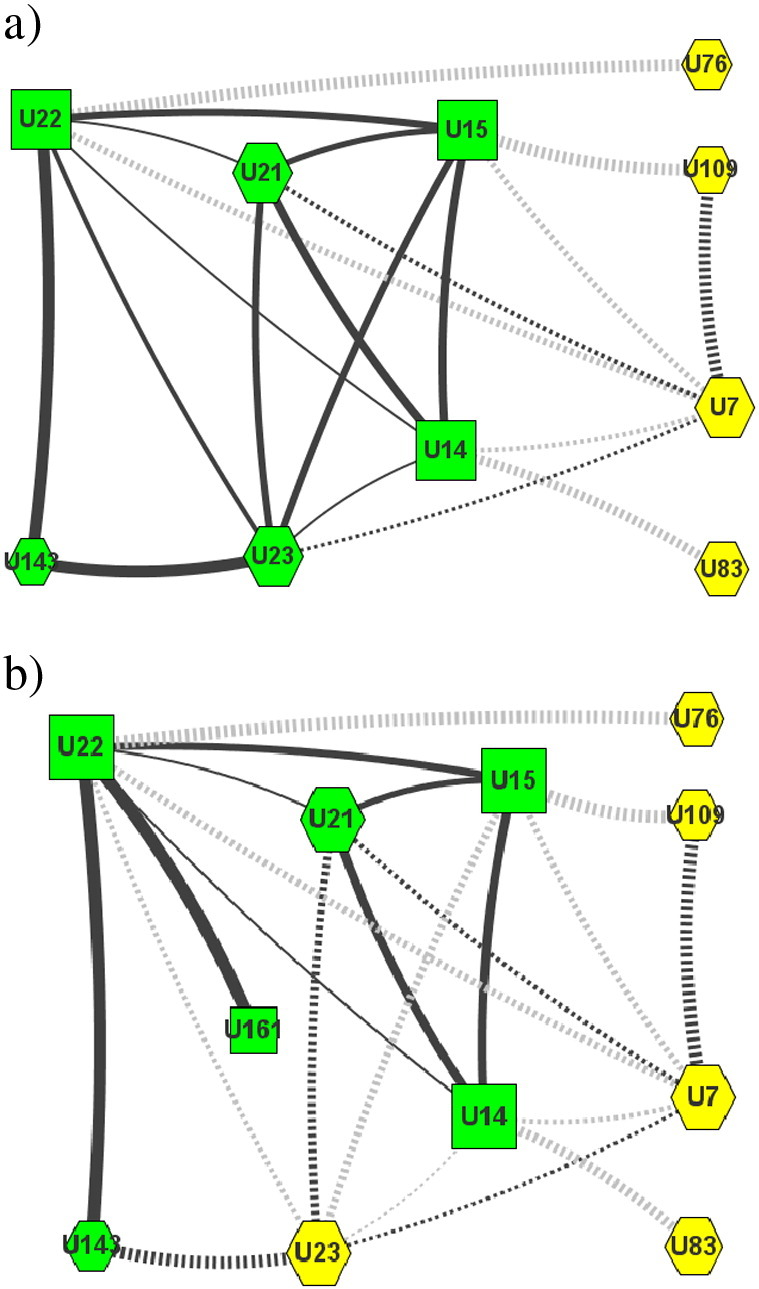
Team formation result with Genetic Algorithms (a) and Simulated Annealing (b) from Experiment 1.2, 40% unavailable experts, using dynamic γ for trade-off between W_e and W_r. Full edges between best team members (green squares, and hexagons), dashed edges between Top Team members (yellow hexagons). Thicker edges represent tighter links.

Table 3.

Top Team and best teams generated by Genetic Algorithm and Simulated Annealing for an example simulated team formation from Experiment 1.2.

Skill	Top Team	T(GA)	q(s)	T(SA)	q(s)
S0	U7	U21	0.71	U161	0.53
S1	U21	U15	0.86	U15	0.86
S2	U23	U23	1.00	U15	0.67
S3	U23	U23	1.00	U14	0.47
S4	U109	U14	0.79	U21	0.79
S5	U83	U23	0.87	U14	0.91
S6	U76	U22	0.70	U22	0.70
S7	U143	U143	1.00	U143	1.00
Coverage		0.87		0.74
Distance		0.45		0.60
Energy		0.46		0.63
Quality		2.17		1.58

Both heuristics exploit the composition restriction (minimum 6 experts) to the full extent and reduce the initial number of involved experts. The genetic algorithm preserves three members from the Top Team ([U21, U23, U143]) but assigns U21 a different skill. All three additional members come with high skills (q(s) ≥ 0.7) and considerably reduce the team distance. The normalized team density is comparatively high with 0.893 due to U23 and U22 linking to every other member, and only U143 featuring less than three intra-team relations. Simulated annealing improves similarly on distance, but not as successfully. Two members from the Top Team U21 and U143 join 4 new members all having skills higher than 0.45. The lower normalized team density of 0.607 is largely due to two experts (U143 and U161) having only a single link, and only a single expert (U22) yielding previous interactions with all other members.

In direct comparison, the genetic algorithm manages to maintain higher coverage while achieving lower distance than simulated annealing. Inverting the energy metric we obtain the team quality: GA more than doubles the team quality, whereas GA provides only a 58% increase (compared to the Top Team that has quality and energy always equal to 1). Teams produced by GA and SA highlight a general property of the formation process: at least some members of the Top Team will always be part of the best found team. In this example, GA and SA produced rather similar final teams (overlap of 5 members). Later in Section 7.5.1 we test for correlation of GA and SA to determine if this is usually the case.

7.5. Comparing GA and SA for dynamic γ

In our experiments, the GA consistently outperforms SA. Fig. 16 compares the average fitness values for the best final teams. For full expert availability the genetic algorithm delivers a 2.3× to 3.5× fitness improvement compared to the initial Top Team. SA in contrast increases fitness only by a factor 1.1× to 1.9×. The difference becomes smaller with declining γ. For 40% unavailable experts, GA improves fitness by 38% to 92%, whereas SA ranges between 37% and 68% respectively. Looking in more detail at coverage and distance, we note that the GA performs better at finding densely connected teams while maintaining consistently high coverage.

Fig. 16.

Average fitness of the best final teams produced by Simulated Annealing (boxes) and Genetic Algorithm (circles).

For both heuristics, coverage $\mathcal{C}$ remains comparatively high regardless of the amount of available expert, even though we have put more focus on achieving lower distance than high coverage (α  = 0.1). Across all experiments and both heuristics, average coverage resides above 0.6 even though we have set the lower limit for expertise to q(s)_min  = 0.2. SA produces teams with higher coverage than GA but simultaneously delivers smaller distance improvements.

When applying genetic algorithms, distance $\mathcal{D}$ decreases linearly and converges to roughly the same level as simulated annealing as an increasing number of experts become unavailable. GA thus clearly outperforms SA below 30% unavailable experts. Given the large standard deviation in distance improvements and also coverage, the results are closer together for 30% and 40% missing experts. While SA failed to produce a better final team than Top(${\mathcal{S}}_{\mathcal{R}}$) 25× across 150 experiment rounds (50 rounds each in Ex 1.1, 1.2, and 2), GA only failed to do so 6×. This also explains Simulated Annealing's spike in distance improvement for 10% and 20% in Experiment 2 when 3 out of 10 team configurations could not be improved.

7.5.1. Heuristic correlation

As indicated by the error bars in Fig. 17 , both heuristics yield a significant amount of deviation in distance improvements and also coverage. We therefore test these two metrics for correlation to determine if one heuristic performs better in cases where the other heuristic performs poorly and vice versa and thus complement each other.

Comparing SA and GA with the pearson correlation coefficient, we specify the null hypothesis ρ  = 0 for all experiment sets. We obtain following values for coverage (ρ _Ex1.1  = 0.27; ρ _Ex1.2  = 0.14; ρ _Ex2  = 0.41), and distance improvement (ρ _Ex1.1  = 0.8; ρ _Ex1.2  = 0.43; ρ _Ex2  = 0.11). With sampling size 50 and a significance level for two-tailed test of 0.01, ρ needs to be greater than 0.354 to be significantly different from zero, respectively ρ needs to be smaller than − 0.354 for inverse correlation. Hence, we accept the null hypothesis for coverage (Ex 1.1, Ex 2) and distance improvement (Ex 1.1, Ex 2) that there exist no correlation between GA and SA. There is even a small, but significant relationship between SA and GA for distance improvement in Experiment 1.2 and coverage in Experiment 2. Given these correlation measurements there is no evidence that the two heuristics complement each other.

In addition we inspect the few instances where GA or SA was unable to find better teams than the initial Top Team. As mentioned above, GA failed to do so 6×, while SA failed 25×. Out of the 6 unsuccessful GA attempts, SA similarly did not provide a better solution and provided only little improvement for the remaining 2 attempts. In contrast, GA found significantly better teams for the remaining 19 SA misses. This supports the correlation measurement above: simulated annealing and the genetic algorithm are not complementary.

7.5.2. Comparison to real-world data

We compare the data generated by our experiment model and a real-world data set to validate our results. Slashdot is an IT-centric news site where each posted story receives extensive discussions. A reply posting between two comment authors becomes an interaction link. The skills are extracted from a news story's subdomain. We derived an expert network from the Slashdot postings from January 1st 2008 to June 30th 2008, covering the subdomains apple, ask, entertainment, mobile, linux, developers, games, news, slashdot, and it. We didn't, however, run detailed team formation experiments on the Slashdot data set as the number of available skills is limited and thus does not allow for sufficient experiment variations necessary to generate reliable results.

General social network characteristics of the Slashdot postings are discussed in [20]. In this paper, we focus on the correlation of degree and expertise to demonstrate that our simulation model correctly reproduces real-world settings. In addition we compare the effect of unavailable experts on the candidate network density. Fig. 18 depicts the degree of an expert printed against his/her total expertise score q(∙). The compared data sets comprise the two networks used in the evaluation (blue circle, green plus), a larger synthetic set (10,000 experts, red crosses) and the Slashdot data set of 12,000 experts (purple squares). All four data sets derive from a different overall skill, required skill, and expert count configuration,¹⁰ yet we observe in every case a linear correlation between degree and score. The slope is defined by the amount of required skills (theoretical maximum score is the amount of skills) and the maximum degree.

Fig. 18.

Degree vs. Score for synthetic network of 200, 1000, and 10,000 nodes and Slashdot with 12,000 nodes.

The power-law network topology has a profound effect on the results of our team formation algorithm. The strategy for marking experts as unavailable directly affects the connectivity of the observed candidate network. Degree-based availability reduces the connectivity rapidly as predominantly well connected experts are marked as overloaded. Here γ drops from 0.75, respectively from 1, to 0.39. Already with 10% (Experiment 1), respectively 20% (Experiment 2), of experts unavailable, γ is below 0.6. The effect of degree-based node removal in power-law networks is well analyzed (e.g., [60]) but briefly repeated here to highlight its significance on the trade-off between interaction-based and recommendation-based team formation.

We visualize the effect of expert unavailability on γ in Fig. 19 . The complete Slashdot network (purple squares) comprises 8 out of 10 skills from 12,000 experts. A second network (a subset of the complete Slashdot expert network (red triangles)) contains 6 skills, from which we select 5 to generate the candidate network. Degree preferential selection of Slashdot experts shows an even more swift decrease in density than our model: γ drops in both Slashdot data sets below 0.4 when removing 10% of experts and then converges to 0.05. We have to assume an inverse rich-club effect, stronger than in our model. Thus we can safely assume that a trade-off between interaction and recommendation-based distance is even more significant in real world expert crowds.

Fig. 19.

Effect of increasingly unavailable experts on γ for synthetic and Slashdot networks.

8. Conclusion

Team composition requires a balance between maintaining sufficiently high skill coverage and adequately connected team members. Finding a suitable team for a given trade-off between skills and connectivity is NP complete. The problem is further aggravated in crowds as the top experts are most popular and thus become easily overloaded. The social network structure of crowds usually lacks a rich-club structure. When a small fraction of top experts (≈ 10%) becomes unavailable, the social network becomes too sparse to compose a team based on direct interactions alone. We thus propose to apply skill-dependent recommendations to substitute direct interactions. In addition, the introduced team-centric recommendation model considers only the recommendations of the team members' common neighbors. Our approach then analyzes network density to dynamically adjust the importance of direct interactions compared to recommendations.

Genetic Algorithms and Simulated Annealing are two suitable heuristics to address the multi-objective team composition problem. Genetic Algorithms apply cross over and mutation of team configurations to approach the best team while Simulated Annealing relies on a cooling schedule. Experiments have successfully shown that both heuristics are able to find significantly better solutions than the simple set of top ranked experts. The Genetic Algorithm, however, produced better and more stable results, especially for smaller networks. Analysis of increasingly unavailable experts demonstrated that our trade-off model accurately guides the transition from direct interaction links to recommendations. Consequently the composition mechanism focuses on direct links as long as possible before experts are integrated into the team based on recommendations. Such dynamic adaptation enables us to obtain teams that yield both higher recommendations and lower distance than the initial top team. Ultimately we were able to obtain team configurations that exhibit desirably low team distance, while maintaining consistently high skill coverage even when removing up to 40% experts from the social network.

We intend to continue our research in multiple directions. First, we plan to evaluate our approach with other real-world data sets which exhibit a larger skill set. The DBLP dataset is one possible candidate. This effort however has to go in hand with a rigorous analysis of skill distribution and therefore was not attempted in the scope of this work. Second, we intend to investigate how to exploit interaction patterns [61] to more accurately interpret the link strength between experts. Finally, we expect exciting results from exploring how our approach can enhance existing work on team-aware process management [62] in terms of composing an optimal team for executing a process.

Biographies

Christoph Dorn received his MSocEcSc (Magister) in Business Informatics in 2004, and his Ph.D in Computer Science (Dr. techn.) in 2009, both from the Vienna University of Technology. After working as a Post-Doc researcher at the Distributed Systems Group, he is now a visiting researcher with an FWF Schroedinger Mobility Fellowship at the Institute for Software Research at the University of California , Irvine. His research interests cover context-aware computing, people-driven ad-hoc workflows, Web service adaptation, social network analysis, and collaborative working environments. More information at: http://christophdorn.wordpress.com.

Florian Skopik is a postdoctoral researcher at the Vienna University of Technology. He received his PhD in June 2010 with a thesis on “Dynamic Trust in Mixed Service-oriented Systems” while working as a research assistant at the Distributed Systems Group, Vienna University of Technology. His research interests include models, algorithms and architectures that support the management of trust in social and collaborative service-oriented environments. More information can be found at http://www.infosys.tuwien.ac.at/Staff/skopik.

Daniel Schall is a postdoctoral researcher at the Vienna University of Technology. He defended his PhD in February 2009 with a thesis on “Human Interactions in Mixed Systems — Architecture, Protocols, and Algorithms” while working as a research assistant at the Distributed Systems Group, Vienna University of Technology. Prior to joining the Distributed Systems Group, he worked at Siemens Corporate Research in Princeton, New Jersey, USA. More information can be found at http://www.infosys.tuwien.ac.at/staff/dschall/.

Schahram Dustdar is a full professor of computer science (informatics) with a focus on Internet technologies and head of the Distributed Systems Group at the Vienna University of Technology (TU Wien). He has published some 250 scientific papers as conference-, journal-, and book contributions. He co-organized several scientific workshops and conferences (such as ICSOC 2007 and BPM 2006) and has been serving on more than 200 international program committees as well as on editorial boards of 10 scientific journals. Dustdar is an ACM Distinguished Scientist. More information at: www.infosys.tuwien.ac.at/Staff/sd.

Annex A. Extended experiment results

Fig. 20

References

- 1.Brabham D. Crowdsourcing as a model for problem solving: an introduction and cases. Convergence. 2008;14(1):75. [Google Scholar]
- 2.Fitzpatrick E.L., Askin R.G. Forming effective worker teams with multi-functional skill requirements. Computers and Industrial Engineering. 2005;48(3):593–608. doi: http://dx.doi.org/10.1016/j.cie.2004.12.014. [Google Scholar]
- 3.Wi H., Oh S., Mun J., Jung M. A team formation model based on knowledge and collaboration. Expert Systems with Applications. 2009;36(5):9121–9134. doi: http://dx.doi.org/10.1016/j.eswa.2008.12.031. [Google Scholar]
- 4.Baykasoglu A., Dereli T., Das S. Project team selection using fuzzy optimization approach. Cybernetics and Systems. 2007;38(2):155–185. doi: http://dx.doi.org/10.1080/01969720601139041. [Google Scholar]
- 5.Cheatham M., Cleereman K. CTS '06: Proceedings of the International Symposium on Collaborative Technologies and Systems. IEEE Computer Society; Washington, DC, USA: 2006. Application of social network analysis to collaborative team formation; pp. 306–311. doi: http://dx.doi.org/10.1109/CTS.2006.18. [Google Scholar]
- 6.Sozio M., Gionis A. Proceedings of the 16th ACM SIGKDD international conference on Knowledge discovery and data mining, KDD '10. ACM; New York, NY, USA: 2010. The community-search problem and how to plan a successful cocktail party; pp. 939–948.http://doi.acm.org/10.1145/1835804.1835923 [Google Scholar]
- 7.Anagnostopoulos A., Becchetti L., Castillo C., Gionis A., Leonardi S. Proceedings of the 19th ACM international conference on Information and knowledge management, CIKM '10. ACM; New York, NY, USA: 2010. Power in unity: forming teams in large-scale community systems; pp. 599–608.http://doi.acm.org/10.1145/1871437.1871515 [Google Scholar]
- 8.Yang D.-N., Chen Y.-L., Lee W.-C., Chen M.-S. Vol. 4. 2011. On social-temporal group query with acquaintance constraint; pp. 397–408.http://portal.acm.org/citation.cfm?id=1978665.1978671 (Proc. VLDB Endow). [Google Scholar]
- 9.Craig M., Horton D., Pitt F. Proceedings of the 16th ACM international conference on Supporting group work, GROUP '10. ACM; New York, NY, USA: 2010. Forming reasonably optimal groups: (frog) pp. 141–150.http://doi.acm.org/10.1145/1880071.1880094 [Google Scholar]
- 10.Xie M., Lakshmanan L.V., Wood P.T. Proceedings of the fourth ACM conference on Recommender systems, RecSys '10. ACM; New York, NY, USA: 2010. Breaking out of the box of recommendations: from items to packages; pp. 151–158.http://doi.acm.org/10.1145/1864708.1864739 [Google Scholar]
- 11.Datta A., Tan Teck Yong J., Ventresque A. Proceedings of the 20th international conference companion on World wide web, WWW '11. ACM; New York, NY, USA: 2011. T-recs: team recommendation system through expertise and cohesiveness; pp. 201–204.http://doi.acm.org/10.1145/1963192.1963289 [Google Scholar]
- 12.Fortunato S. Co mmunity detection in graphs. Physics Reports. 2010;486(3–5):75–174. http://www.sciencedirect.com/science/article/pii/S0370157309002841 [Google Scholar]
- 13.Lappas T., Liu K., Terzi E. KDD '09: Proceedings of the 15th ACM SIGKDD Int. Conference on Knowledge discovery and data mining. ACM; New York, NY, USA: 2009. Finding a team of experts in social networks; pp. 467–476. doi: http://doi.acm.org/10.1145/1557019.1557074. [Google Scholar]
- 14.Singh P.V. The small-world effect: the influence of macro-level properties of developer collaboration networks on open-source project success. ACM Transactions on Software Engineering and Methodology. 2010;20:6:1–6:27. http://doi.acm.org/10.1145/1824760.1824763 [Google Scholar]
- 15.Gaston M.E., Simmons J., desJardins M. AAMAS-04 Workshop on Learning and Evolution in Agent Based Systems. 2004. Adapting network structure for efficient team formation. [Google Scholar]
- 16.Chen C.-C. Intelligent Networking and Collaborative Systems (INCOS), 2010 2nd International Conference on, 2010. 2010. A multi-level study of free-loading in dynamic groups: the importance of initial network topology; pp. 16–23. [Google Scholar]
- 17.Backstrom L., Huttenlocher D., Kleinberg J., Lan X. KDD '06: Proceedings of the 12th ACM SIGKDD international conference on Knowledge discovery and data mining. ACM; New York, NY, USA: 2006. Group formation in large social networks: membership, growth, and evolution; pp. 44–54. doi: http://doi.acm.org/10.1145/1150402.1150412. [Google Scholar]
- 18.McAuley J.J., da Fontoura Costa L., Caetano T.S. Rich-club phenomenon across complex network hierarchies. Applied Physics Letters. 2007;91(8):084103. [Google Scholar]
- 19.Colizza V., Flammini A., Serrano M.A., Vespignani A. Detecting rich-club ordering in complex networks. Nature Physics. 2006;2:110–115. [Google Scholar]
- 20.Gómez V., Kaltenbrunner A., López V. WWW '08: Proceedings of the 17th Int. Conference on World Wide Web. ACM; New York, NY, USA: 2008. Statistical analysis of the social network and discussion threads in slashdot; pp. 645–654. doi: http://doi.acm.org/10.1145/1367497.1367585. [Google Scholar]
- 21.Adamic L.A., Zhang J., Bakshy E., Ackerman M.S. WWW '08: Proceeding of the 17th Int. Conference on World Wide Web. ACM; New York, NY, USA: 2008. Knowledge sharing and yahoo answers: everyone knows something; pp. 665–674. doi: http://doi.acm.org/10.1145/1367497.1367587. [Google Scholar]
- 22.Bird C., Gourley A., Devanbu P., Gertz M., Swaminathan A. MSR '06: Proceedings of the 2006 Int. Workshop on Mining software repositories. ACM Press; New York, NY, USA: 2006. Mining email social networks; pp. 137–143. doi: http://doi.acm.org/10.1145/1137983.1138016. [Google Scholar]
- 23.Chundi P., Subramaniam M., Vasireddy D.K. An approach for temporal analysis of email data based on segmentation. Data & Knowledge Engineering. 2009;68:1253–1270. http://www.sciencedirect.com/science/article/B6TYX-4WB3N78-1/2/ca0fcdcf7cccd593416a6c32092cad23 including Special Section: Conference on Privacy in Statistical Databases (PSD 2008) — Six selected and extended papers on Database Privacy. [Google Scholar]
- 24.Bird C., Pattison D., D'Souza R., Filkov V., Devanbu P. SIGSOFT '08/FSE-16: Proceedings of the 16th ACM SIGSOFT International Symposium on Foundations of software engineering. ACM; New York, NY, USA: 2008. Latent social structure in open source projects; pp. 24–35. doi: http://doi.acm.org/10.1145/1453101.1453107. [Google Scholar]
- 25.Duan D., Li Y., Jin Y., Lu Z. Proceeding of the 1st ACM international workshop on Complex networks meet information & knowledge management, CNIKM '09. ACM; New York, NY, USA: 2009. Community mining on dynamic weighted directed graphs; pp. 11–18.http://doi.acm.org/10.1145/1651274.1651278 [Google Scholar]
- 26.Provost F., Dalessandro B., Hook R., Zhang X., Murray A. Proceedings of the 15th ACM SIGKDD international conference on Knowledge discovery and data mining, KDD '09. ACM; New York, NY, USA: 2009. Audience selection for on-line brand advertising: privacy-friendly social network targeting; pp. 707–716.http://doi.acm.org/10.1145/1557019.1557098 [Google Scholar]
- 27.Dong Z., Song G., Xie K., Sun Y., Wang J. Proceedings of the 6th international conference on Fuzzy systems and knowledge discovery — Volume 5, FSKD'09. IEEE Press; Piscataway, NJ, USA: 2009. Adequacy of data for mining individual friendship pattern from cellular phone call logs; pp. 573–577.http://portal.acm.org/citation.cfm?id=1801874.1801997 [Google Scholar]
- 28.Bouguessa M., Wang S., Dumoulin B. Discovering knowledge-sharing communities in question-answering forums. ACM Transactions on Knowledge Discovery from Data. 2010;5:3:1–3:49. http://doi.acm.org/10.1145/1870096.1870099 [Google Scholar]
- 29.Dustdar S., Schreiner W. A survey on web services composition. International Journal of Web and Grid Services. 2005;1(1):1–30. doi: http://dx.doi.org/10.1504/IJWGS.2005.007545. [Google Scholar]
- 30.Yang Y., Mahon F., Williams M.H., Pfeifer T. Context-aware Dynamic Personalised Service Re-composition in a Pervasive Service Environment. UIC; 2006. pp. 724–735. [Google Scholar]
- 31.Quitadamo R., Zambonelli F., Cabri G. Software Engineering for Pervasive Computing Applications, Systems, and Environments, 2007. 2007. The service ecosystem: dynamic self-aggregation of pervasive communication services; pp. 1–10. (SEPCASE '07. First International Workshop on, 2007). [Google Scholar]
- 32.Maamar Z., Benslimane D., Thiran P., Ghedira C., Dustdar S., Sattanathan S. Towards a context-based multi-type policy approach for web services composition. Data & Knowledge Engineering. 2007;62(2):327–351. doi: http://dx.doi.org/10.1016/j.datak.2006.08.007. [Google Scholar]
- 33.Baresi L., Bianchini D., Antonellis V.D., Fugini M.G., Pernici B., Plebani P. Context-aware Composition of E-services. TES; 2003. pp. 28–41. [Google Scholar]
- 34.Brin S., Page L. The anatomy of a large-scale hypertextual web search engine. Computer Networks and ISDN Systems. 1998;30(1–7):107–117. [Google Scholar]; proceedings of the Seventh International World Wide Web Conference. doi: 10.1016/S0169-7552(98)00110-X
- 35.Haveliwala T. Topic-sensitive pagerank: a context-sensitive ranking algorithm for web search. IEEE Transactions on Knowledge and Data Engineering. 2003;15(4):784–796. [Google Scholar]
- 36.Balog K., De Rijke M. Proceedings of the 20th international joint conference on Artifical intelligence. Morgan Kaufmann Publishers Inc.; San Francisco, CA, USA: 2007. Determining expert profiles (with an application to expert finding) pp. 2657–2662.http://portal.acm.org/citation.cfm?id=1625275.1625703 [Google Scholar]
- 37.Horowitz D., Kamvar S.D. Proceedings of the 19th international conference on World wide web, WWW '10. ACM; New York, NY, USA: 2010. The anatomy of a large-scale social search engine; pp. 431–440.http://doi.acm.org/10.1145/1772690.1772735 [Google Scholar]
- 38.Schall D., Dustdar S. Dynamic context-sensitive pagerank for expertise mining. In: Bolc L., Makowski M., Wierzbicki A., editors. SocInfo, Vol. 6430 of Lecture Notes in Computer Science. Springer; 2010. pp. 160–175. [Google Scholar]
- 39.Bonchi F., Castillo C., Gionis A., Jaimes A. Social network analysis and mining for business applications. ACM Transactions on Intelligent Systems and Technology. 2011;2:22:1–22:37. http://doi.acm.org/10.1145/1961189.1961194 [Google Scholar]
- 40.Liben-Nowell D., Kleinberg J. International Conference on Information and Knowledge Management. ACM; 2003. The link prediction problem for social networks; pp. 556–559. [Google Scholar]
- 41.Hang C.-W., Singh M.P. 13th AAMAS Workshop on Trust in Agent Societies (Trust) 2010. Trust-based recommendation based on graph similarity. [Google Scholar]
- 42.Skopik F., Schall D., Dustdar S. Modeling and mining of dynamic trust in complex service-oriented systems. Information Systems. 2010;35(7):735–757. doi: http://dx.doi.org/10.1016/j.is.2010.03.001. [Google Scholar]
- 43.Falahi K., Atif Y., Elnaffar S. Green Computing and Communications (GreenCom), 2010 IEEE/ACM Int'l Conference on Int'l Conference on Cyber, Physical and Social Computing (CPSCom) 2010. Social networks: challenges and new opportunities; pp. 804–808. [Google Scholar]
- 44.Caverlee J., Liu L., Webb S. Proceeding of the 17th international conference on World Wide Web, WWW '08. ACM; New York, NY, USA: 2008. Towards robust trust establishment in web-based social networks with socialtrust; pp. 1163–1164.http://doi.acm.org/10.1145/1367497.1367707 [Google Scholar]
- 45.Sirivianos M., Kim K., Yang X. Proceedings of the 4th USENIX conference on Hot topics in security, HotSec'09. USENIX Association; Berkeley, CA, USA: 2009. Facetrust: assessing the credibility of online personas via social networks; p. 2-2.http://portal.acm.org/citation.cfm?id=1855628.1855630 [Google Scholar]
- 46.D. Schall, Human interactions in mixed systems — architecture, protocols, and algorithms, PhD Thesis, Vienna University of Technology, Karlsplatz 13, 1040 Vienna, Austria (2009).
- 47.Suman B., Kumar P. A survey of simulated annealing as a tool for single and multiobjective optimization. The Journal of the Operational Research Society. 2005;57(10):1143–1160. http://www.palgrave-journals.com/doifinder/10.1057/palgrave.jors.2602068 [Google Scholar]
- 48.Deb K. 1st edition. Wiley; 2001. Multi-Objective Optimization using Evolutionary Algorithms. [Google Scholar]
- 49.Srinivas M., Patnaik L. Adaptive probabilities of crossover and mutation in genetic algorithms. IEEE Transactions on Systems, Man, and Cybernetics. 1994;24(4):656–667. [Google Scholar]
- 50.Zhang J., Chung H.S.-H., Lo W.-L. Clustering-based adaptive crossover and mutation probabilities for genetic algorithms. IEEE Transactions on Evolutionary Computation. 2007;11(3):326–335. [Google Scholar]
- 51.Jong K.A.D., Spears W.M. Proceedings of the 1st Workshop on Parallel Problem Solving from Nature, PPSN I. Springer-Verlag; London, UK: 1991. An analysis of the interacting roles of population size and crossover in genetic algorithms; pp. 38–47.http://portal.acm.org/citation.cfm?id=645821.670188 [Google Scholar]
- 52.Weyland D. Proceedings of the 10th annual conference on Genetic and evolutionary computation, GECCO '08. ACM; New York, NY, USA: 2008. Simulated annealing, its parameter settings and the longest common subsequence problem; pp. 803–810.http://doi.acm.org/10.1145/1389095.1389253 [Google Scholar]
- 53.Park M.-W., Kim Y.-D. A systematic procedure for setting parameters in simulated annealing algorithms. Computers and Operations Research. 1998;25(3):207–217. http://www.sciencedirect.com/science/article/B6VC5-3SX6XDK-5/2/59aefca9874d9f2a4458c44aba791670 [Google Scholar]
- 54.Orsila H., Salminen E., Hämäläinen T.D. Proceedings of the 11th international conference on System-on-chip, SOC'09. IEEE Press; Piscataway, NJ, USA: 2009. Parameterizing simulated annealing for distributing kahn process networks on multiprocessor socs; pp. 19–26.http://portal.acm.org/citation.cfm?id=1736530.1736534 [Google Scholar]
- 55.Deb K., Pratap A., Agarwal S., Meyarivan T. A fast and elitist multiobjective genetic algorithm: Nsga-ii. IEEE Transactions on Evolutionary Computation. 2002;6(2):182–197. [Google Scholar]
- 56.Fredman M., Tarjan R. Foundations of Computer Science, Annual IEEE Symposium on 0. 1984. Fibonacci heaps and their uses in improved network optimization algorithms; pp. 338–346. doi: http://doi.ieeecomputersociety.org/10.1109/SFCS.1984.715934. [Google Scholar]
- 57.Albert R., Jeong H., Barabasi A. The diameter of the world wide web. CoRR cond-mat/9907038. 1999 [Google Scholar]
- 58.Albert R., Barabasi A.-L. St atistical mechanics of complex networks. Reviews of Modern Physics. 2002;74:47. http://www.citebase.org/abstract?id=oai:arXiv.org:cond-mat/0106096 [Google Scholar]
- 59.Barabasi A., Albert R. Emergence of scaling in random networks. Science. 1999;286:509–512. doi: 10.1126/science.286.5439.509. [DOI] [PubMed] [Google Scholar]
- 60.Callaway D.S., Newman M.E.J., Strogatz S.H., Watts D.J. Network robustness and fragility: percolation on random graphs. Physical Review Letters. 2000;85(25):5468–5471. doi: 10.1103/PhysRevLett.85.5468. [DOI] [PubMed] [Google Scholar]
- 61.Dustdar S., Hoffmann T. Interaction pattern detection in process oriented information systems. Data & Knowledge Engineering. 2007;62(1):138–155. http://www.sciencedirect.com/science/article/B6TYX-4KRY749-1/2/10ace51a52186445e4c1048f911d4f35 [Google Scholar]
- 62.van der Aalst W.M.P., Kumar A. A reference model for team-enabled workflow management systems. Data & Knowledge Engineering. 2001;38(3):335–363. http://www.sciencedirect.com/science/article/B6TYX-4447T69-4/2/7fc8ebe39be4d6a51301e9ff1f294e76 [Google Scholar]