(φ,ψ)₂-motifs: a purely conformation-based, fine-grained enumeration of protein parts at the two-residue level

Abstract

A deep understanding of protein structure benefits from the use of a variety of classification strategies that enhance our ability to effectively describe local patterns of conformation. Here, we use a clustering algorithm to analyze 76,533 all-trans segments from protein structures solved at 1.2 Å resolution or better to create a purely φ,ψ-based comprehensive empirical categorization of common conformations adopted by two adjacent φ,ψ-pairs (i.e. (φ,ψ)₂-motifs). The clustering algorithm works in an origin-shifted 4-dimensional space based on the two φ,ψ-pairs to yield a parameter-dependent list of (φ,ψ)₂-motifs – in order of their prominence. The results are remarkably distinct from and complementary to the standard hydrogen-bond centered view of secondary structure. New insights include an unprecedented level of precision in describing the φ,ψ-angles of both previously known and novel motifs, an ordering of these motifs by their population density, a data-driven recommendation that the standard Cα_i…Cα_i+3 < 7 Å criteria for defining turns be changed to 6.5 Å, an identification of β-strand and turn capping motifs, and of conformational capping by residues in the polypeptide-II (P_II) conformation. We further document that the conformational preferences of a residue are substantially influenced by the conformation of its neighbors, and suggest that accounting for these dependencies will improve protein modeling accuracy. Although the CUEVAS-4D(r₁₀є₁₄) “parts list” presented here is only an initial exploration of the complex (φ,ψ)₂-landscape of proteins, it shows there is value to be had from this approach and opens the door to more in-depth characterizations at the (φ,ψ)₂-level and at higher dimensions.

Introduction

The tertiary structure of folded proteins is constructed from short segments that have been described as “a small catalog of recognizable parts that fit together in a limited number of ways”¹. The phrase “secondary structure” was originally used to account for the α-helix² and the β-strand³, both of which are simple linear groups (based on a single repeating conformation) that allow for regular backbone hydrogen-bonding. We have recently shown that based on ultra-high resolution structures these two motifs plus the 3₁₀-helix⁴ and the polypeptide-II (polyproline-II or P_II) spiral first seen in collagen⁵ are the only linear groups in proteins⁶.

As the first protein structures were solved, it was realized that four-residue hydrogen-bonded tight turns¹ could be considered a kind of secondary structure even though they were not built from a single repeating conformation. Assuming trans-peptide bonds and using φ,ψ-angles, a then newly developed tool for describing polypeptide conformation^{7; 8}, Venkatachalam⁹ enumerated possible tight turns by considering all combinations of the φ,ψ-pairs of two adjacent residues (what we will here call a (φ,ψ)₂-conformation)¹⁰. That survey delineated just six types of hydrogen-bonded tight turns (Types I, II, III and their mirror images I’, II’ and III’). The tight turn definition was later relaxed to include all non-α-helical conformations placing the Cα-atoms of the first and fourth residues within 7 Å of one another¹¹ whether or not a local hydrogen-bond was formed. Today, a protein’s secondary structure tends to be described in terms of α and 3₁₀-helices, β-strands, and tight turns. Anything not fitting one of these categories (even including P_II-spirals) tends to be grouped together as ‘coil’ or even ‘random coil’ even though these segments are quite non-random.

Over time, secondary structural analyses have continued to be largely based on hydrogen-bonding patterns and additional tight turns¹², gamma turns¹³, β-bulges¹⁴, helix caps¹⁵ and coil motifs¹⁶ have been recognized as common features of protein structure, contributing to a growing body of knowledge once comprehensively described as “The Anatomy and Taxonomy of Protein Structure.”¹⁷ As the database of protein structures has grown and computational tools have been developed, many further efforts have been made to organize, categorize, and discover protein building blocks. The very successful fragment-based approaches to protein structure prediction and model-building do not attempt to describe the building blocks, but effectively organize real fragments of protein structures for use in modeling^18-20.

Other approaches to identify and describe common motifs have involved machine-learning strategies^{10; 21-30}. Whereas each such study produced unique insights and some identified specific new motifs, none of these have been comprehensive and detailed, purely conformation-based studies. The studies by design produced selective rather than comprehensive results (e.g. by focusing on subsets of protein structure such as only coil residues, only turns, only helix caps or only non-Gly residues) and/or the studies mixed diverse conformations into single groups (e.g. by grouping conformations into very broad φ,ψ-regions or categorizing residues based on secondary structural states, hydrogen-bonding features, hydrophobic side-chain packing interactions or Cα-positions). Also to have a large enough dataset size to analyze, most previous studies used a resolution limit set at 2.0 Å or worse. A typical 2 Å resolution protein structure has a residual coordinate uncertainty of ~0.3 Å (e.g. Brunger 1997)³¹, degrading the ability to precisely define conformational features.

Ultra-high (≤1.2 Å) resolution protein structures typically have coordinate uncertainties of <0.05 ų², and there are now enough such structures to revisit basic questions of protein conformation. We have begun down this road by creating a Protein Geometry Database (PGD)³³ as a resource for studying protein conformation, covalent geometry and their interrelationships. We have already used the PGD to revisit the question of what linear groups exist in protein structures⁶ and to map out the details of how protein covalent geometry varies as a function of conformation³⁴. Here, we use an automated clustering protocol to present a purely conformation-based analysis of (φ,ψ)₂-conformations as seen in a ~75,000 residue dataset from protein structures refined at 1.2 Å resolution or better. In this analysis, we first select a strategy and parameters that will yield an appropriate level of discrimination, and then use these parameters to identify a comprehensive set of (φ,ψ)₂-motifs, which are ranked by relative prominence and assessed for their secondary-structure and sequence features.

Results and Discussion

Dataset and Ramachandran Nomenclature

Assuming all trans peptide bonds, the φ,ψ-angles of two adjacent residues (i.e. φ_i+1, ψ_i+1, φ_i+2, ψi+2) specify the path of three peptide planes and the positions of four Cα-atoms (residues i, i+1, i+2, and i+3) . For clarity, we will call these segments (φ,ψ)₂-segments rather than the more ambiguous monikers of dipeptide (for the two adjacent residues), tripeptide (for the three peptide planes), or tetrapeptide (for the four Cα-atoms) segments. Similarly, segments of defined conformation of other lengths will be identified as (φ,ψ)_n-segments¹⁰.

The dataset used for this study was created by a search of the PGD and consists of 76,533 well-ordered four-residue segments from diverse proteins (each having ≤ 25% sequence identity with any other included protein) as seen in crystal structures refined at 1.2 Å resolution or better (see Methods for further details). For each (φ,ψ)₂-segment, the dataset includes the φ,ψ-angles for the central two residues, the ω–torsion angles for the three peptide units involved, and for all four residues includes the residue types and secondary structures according to DSSP³⁵. To describe the conformations of individual residues in this dataset, we use a nomenclature for φ,ψ-regions based on natural groupings of residues in the Ramachandran plot (Figure 1A; See Hollingsworth & Karplus 2011³⁶), using an assignment grid with 5° pixels (Figure S1). Finally, because accurate clustering depends on having similar conformations be numerically close to one another, it is a problem that the members of some natural groupings are not placed contiguously in a traditional Ramachandran plot – for instance, the β and P_II regions are both split between the top (near ψ =180) and the bottom (near ψ =−180) of the plot (Figure 1A). To minimize this problem, we shifted the ranges of φ and ψ to 0°≤ φ <360° and −100°≤ ψ <240°, respectively. As seen in a plot of this “wrapped” data, no substantially populated natural groupings are divided (Figure 1B, C).

Figure 1.

Ramachandran nomenclature and wrapping. (a) A Ramachandran plot is shown as dots for the conformations of residue i+1 from the 76,533 (φ,ψ)₂-segments used in this study; the shorthand names (based on Hollingsworth & Karplus) and rough outlines for each major natural φ,ψ-grouping are indicated. Also shown are the φ and ψ values that will be used as the origins for the rewrapped data (dashed lines). (b) Same as ‘a’, but using a wrapped Ramachandran plot, with φ_min=0 and ψ_min=−100 to avoid the artificial separation of major groupings, such as the β, ε, P_II, and P_II’ regions. (c) Geo-style 3D wrapped Ramachandran Plot with the z-axis displaying populations in the 76,533 residue high-fidelity dataset. The populations are sums for a series of 20°×20° φ,ψ-bins calculated on a 10° grid. Colors are <25 observations (blue ocean), 26- 75 (sandy beach), 76-500 (vegetated region), and >501 (snowy peaks). See Hollingsworth & Karplus³⁶ for further discussion of the wrapped and 3D plots. This and similar plots were created using Excel 2007 (Microsoft, Redmond).

Conformational clustering using CUEVAS – clustering parameters and strategy

The program CUEVAS³⁷ carries out efficient multi-dimensional clustering of large noisy datasets using the Cuevas-Febrero-Fraiman algorithm³⁸. Based on three user-defined parameters – a data-smoothing radius (r), an observation-density threshold (ρ_th ) reported here in units of points per n-sphere of radius r, and a clustering distance epsilon (є) – CUEVAS converts any set of n-dimensional numerical data into a list of clusters (see Figure 2 and the associated legend). As seen in Figure 2, the result is highly dependent on the parameters used. For instance, for our (φ,ψ)₂ dataset and a low ρ_th corresponding to a single point per sphere of radius r, very large r and є values would result in a single cluster containing all 76,533 observations, whereas extremely small r and є values would result in 76,533 clusters of one observation each.

Figure 2.

A 2-D illustration of the CUEVAS clustering process (a) Step 1: an n-sphere of radius r (as shown) is drawn around each point in the dataset and those having a local observation density greater than the threshold ρ_th are designated as high-density points. (b) Using a ρ_th corresponding to 5 points/circle defines four high-density points (shown). Step 2: all high-density points within є (shown) are grouped into a common cluster using agglomerative clustering. Two clusters identified are shown (blue and red). (c) Using a ρ_th corresponding to 1 point/circle defines all points as high-density points (shown), and using the є from panel ‘b’ results in one supercluster and two other smaller clusters (each uniquely colored). Note how any point further than є away from all other points becomes a cluster of one.

These are uninteresting extremes, and the challenge is to find parameters that result in conceptually informative and practically useful results. We followed a pragmatic approach of selecting parameters that tend to identify known motifs as single clusters, while erring on the side of subdividing known motifs into multiple clusters rather than lumping together motifs that have been considered to be distinct. After many trial runs, we settled on a smoothing radius r=10° and a clustering distance є = 14.1° (i.e. 10√2) for our 4-dimensional (φ,ψ)₂ clustering (see methods).

We do not select a single value for ρ_th, but instead vary it over all possible values following what we call the “Everest strategy” (Figure 3). It is analogous to characterizing the earth’s surface by beginning in the stratosphere and moving slowly towards the center of the earth, listing each feature as it is encountered during the descent (i.e. Mt. Everest would be the first, followed by K2 and so forth with each unique peak identified by its latitude, longitude and peak height ρ_max). As the threshold lowers, a new peak is recognized only if it has a true maximum (i.e. it is not just a rounded shoulder) that is further than є from the closest parts of all other peaks above that threshold. Each identified peak spreads in girth as ρ_th decreases, and as ρ_th drops near the elevations of the valleys separating peaks, those peaks merge together in events we call ‘superclustering.’ Mountains become superclustered into mountain ranges and eventually into continents. A limitation of this approach is that distinct populations that are only rounded shoulders rather than peaks (like conformation II in Figure 3) will be missed.

Figure 3.

Example of the ‘Everest’ approach to motif discovery by CUEVAS. A generic one-dimensional distribution of five conformational motifs (I – V) with the population densities based on a local smoothing using a radius r. With r and є fixed, ρ_th is lowered to identify peaks. At ρth¹, motif III is the only motif identified. At ρth², motifs IV and V are newly identified and the cluster representing motif III expands to include motif II as a shoulder so that motif II is never identified. At ρth³, motifs IV and V supercluster and motif I is discovered. At ρth⁴, motif III/II superclusters together with the motif IV/V cluster, while motif I remains unique.

Clustering of the 4D (φ_i+1, ψ_i+1, φ_i+2, ψ_i+2)-dataset

We applied the Everest strategy with r=10°, є=14.1° to the 76,533 member 4D (φ,ψ)₂-dataset. As seen in Figure 4, there is an explosion of unique clusters at very low thresholds, starting at about ρ_th = 8 and continuing to the nearly 1,500 distinct (by our definitions) isolated clusters with just one member. The clusters occurring at these very low frequencies cannot be considered ‘common’ conformations, so we have chosen ρ_th ≥ 8 as a generous, but manageable threshold for more in-depth description in this initial foray to see what kinds of information this approach can deliver.

Figure 4.

Explosion of unique (φ,ψ)₂-motifs at low thresholds. Shown is a histogram of the total number of novel clusters found at each ρ_th value <15.

Using this ρ_th ≥ 8 cutoff (and r=10°, є=14.1°) yields 101 distinct clusters, or (φ,ψ)₂-motifs, each having a characteristic peak height, ρ_max, and peak (φ_i+1,ψ_i+1,φ_i+2,ψ_i+2)-values. By height (i.e. population density), the clusters range from the α-helix with ρ_max = 12,120 points/sphere down to 15 clusters with ρ_max = 8 points/sphere (Table S1). In terms of (φ,ψ)-angles, the peak values for residues i+1 and i+2 are widely distributed throughout the populated regions of the Ramachandran plot (Figure 5).

Figure 5.

The range of peak positions for (φ,ψ)₂-motifs. Peak positions for residue i+1 (blue squares) and residue i+2 (red triangles) of all 101 (φ,ψ)₂-motifs are included. Motifs with ρ_th> 15 are shown as large, solid symbols and those with a lower ρ_th as small, outlined symbols. Supplementary Figure S4 provides a series of plots connecting the paired residue i+1 and residue i+2 positions.

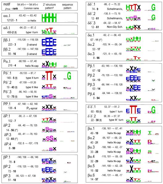
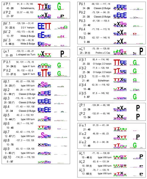
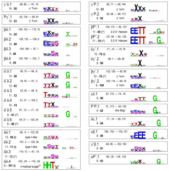
In Table 1 we have grouped these (φ,ψ)₂-motifs by the Ramachandran regions (Figure 1) in which residues i+1 and i+2 reside. In past studies, novel motifs have traditionally been given creative monikers sometimes having little to do with the actual structure. Here we uniquely identified each (φ,ψ)₂-motif by a shorthand descriptor using region names, as suggested by Wilmot & Thornton¹², and an index number based on its relative peak height. For instance, the two most prominent motifs with residue i+1 in the P_II-region and residue i+2 in the δ’-region are designated Pδ’.1 and Pδ’.2. With regards to the Ramachandran region, residues in the α-region have an ambiguity because residues not associated with an α-helix can conceptually be considered part of the extended δ-region (Figure 1). For this reason, for our region-to-region groupings in Table 1, we assigned motifs with α-region φ,ψ-angles as belonging to the δ-region if they were not densely populated (ρ_max <15) and if δ-region motifs with a higher peak height were nearby so the α-region peak was not a dominant feature. Motifs δP.2, δP.3, δδ’.3, and δβ.7 are the four for which this change was made.

Table 1.

The 101 fine-grained (φ,ψ)₂-motifs grouped by region, and their secondary structure and sequence patterns.^a

^aA listing by rank is given in Table S1; Table S2 gives the Cα_i to Cα_i+3 distances; and a series of higher resolution SEQLOGO images are in Figure S5. Using the 10° radius for residues i+1 and i+2, six motif pairs were not completely unique but had a few (up to 4) residues in common: αζ.2 - αζ.3, αζ.2 - αζ.4, δ’β.1 - δ’β.2, δ’β.2 - δ’β.3, δ’δ.2 - δ’δ.4, and δδ.1 - δδ.2.

^bThe secondary structure logos use designators H (α-helix), G (3₁₀-helix), E (β-strand), T (H-bonded turn), S (bend) and X (undesignated). For clarity, ‘X’ rather than a blank represents a residue with no DSSP designated secondary structure, and in the text we call such residues ‘undesignated’ rather than using the misleading ‘coil’ or ‘unstructured’ monikers.

^cInspired by creative naming traditions, we jokingly dubbed this rather unusual motif “the Stig” after a rather unusual TV show character. This motif places the i and i+2 carbonyl oxygens near each other and occurs in loops and a type of β-bulge.

Exploring the natural ranges of select (φ,ψ)₂-motifs

First, we attempted to characterize the sizes and shapes of the (φ,ψ)₂-motifs by allowing the Cuevas algorithm to track the expanding natural range of a cluster as ρ_th drops. As illustrative examples, we show stages in the natural expansion of four of the better-behaved motifs: Pα.1, δ ’δ’.1, Pδ’.1, and P’δ.1 (Figure 6). In these figures, the 4-dimensional cluster distributions are displayed as is commonly done for tight turns, with an arrow connecting the φ,ψ-distributions of the i+1 and i+2 residues in a single Ramachandran plot⁹. In each of these cases it can be seen that as the ρ_th drops, the cluster begins as a sharply defined local region, then grows in a unique manner defining the natural conformational landscape around that peak. As it grows there is first superclustering with near-neighbor motifs to encompass what could at a coarser level be considered as a motif family. Then, as seen in the cases of Pα.1 and Pδ’.1, at still lower ρ_th the cluster becomes much less cohesive as it superclusters with more conformationally distant motifs.

Figure 6.

Examples of natural-range expansion and superclustering of four (φ,ψ)₂-motifs. Observations are shown in black then purple for all residues at the highest two thresholds, and then successively lower thresholds are shown in successively lighter colors, with residue i+1 in blue tones and residue i+2 in red tones. Arrows connect the peak positions (i+1 to i+2) of the (φ,ψ)₂-motifs represented by the spreading populations, with the initially discovered motif shown in green. (a) The spreading of Pα.1 (the P_II conformation helix N-terminal cap) motif at ρ_th values of 159, 61, 30, and 20 and of δ’δ’.1 at ρ_th values 54, 30, 20, and 10. For Pα.1, at ρ_th <16, residue i+1 distributions bridge the gap between the ζ and δ regions to become superclustered with the large α-helix peak. The circled region represents a shoulder motif not discovered by our analysis (see results and discussion). (b) The spreading of the Pδ’.1 (type II turn) motif at ρ_th values of 141, 30, 10, and 5, and of the P’δ.1 (type II’ turn) motif at ρ_th values of 29, 10, and 5.

This visualization of the growth of these four clusters from an initial peak to eventually encompass a wide range of conformations emphasizes the complexity of the (φ,ψ)₂-conformational landscapes, and that there is no absolute standard for deciding for adjoining clusters where one cluster ends and another begins. Indeed, the rapid merging of some neighboring clusters as the threshold is lowered, such as P’δ.1 and P’δ.2 (Figure 6b), provides evidence that our clustering criteria truly do err on the side of subdividing known motifs into multiple clusters, but also raises the question as to whether our criteria are too discriminating and that these motifs would better be considered as a single enlarged motif. In the other direction, the expansion of the Pα.1 motif provides an example (see the circled region in Figure 6a) of a conformationally-distinct shoulder of a higher cluster that is missed by our ‘Everest strategy,’ but would seem by reasonable criteria to represent a (φ,ψ)₂-motif as unique as most others.

Because of complexities like those described above, attempting to define the (φ,ψ)₂-motifs by tracking their natural ranges was too problematic to be of general use. The largest problem was that most of the motifs became superclustered before they accumulated more than a few members. For instance, even the very prominent αδ.1 motif (the type I turn with a peak height of ρth= 499 observations per r=10° 4D-sphere), already merged with αα.1 (the α–helix) motif when it had only 29 high-density observations. In all, only 16 of the 101 motifs accumulated more than 30 members before they merged with other clusters.

Defining fine-grained populations for the 101 (φ,ψ)₂-motifs

Given the inability of the Cuevas clustering algorithm to effectively define large, but discrete non-overlapping populations for each cluster, we used another approach to create a set of precisely and narrowly-defined populations. For each of the identified motifs, we simply culled from the dataset all individual segments having the φ,ψ of residues i+1 and i+2 both within 10° of its motif peak value. We call these populations “fine-grained” (φ,ψ)₂-motifs in contrast to the “natural-range” populations described above. Using this method, each motif has at least eight observations and the number of members is generally one to two times the peak height (exact numbers are in Table S2). This makes sense since the peak height is defined as the population density within an r_4D=10° radius which is somewhat a smaller volume than that defined by two independent r_2D=10° circles. These populations (provided as supplementary data files) were characterized with regard to their DSSP-defined³⁵ secondary structure and amino acid sequence patterns. The secondary structure and sequence patterns results are presented as SEQLOGO³⁹ images to allow essential features to be easily noted and comprehended (Table 1 and Figure S5).

These secondary structure and sequence patterns provide concrete information to evaluate the question raised above of the appropriateness of the level of discrimination we used in defining motifs: if neighboring (φ,ψ)₂-motifs tend to have the highly similar sequence and secondary structure patterns there is no justification for describing them as separate motifs, but the presence of distinct patterns proves that their separation into distinct motifs is appropriate and brings real insight. Considering the P’δ.1 and P’δ.2 pair of (φ,ψ)₂-motifs (Figure 6b) noted above, their separation is justified because their secondary structure patterns are rather distinct, with P’δ.2 predominantly being an isolated turn, very often as part of a β-hairpin, and P’δ.1 rarely associated with a β-hairpin and most often initiating a 3₁₀-helix (Table 1). Similarly, the neighboring Pδ’.1 and Pδ’.2 (φ,ψ)₂-motifs (also in Figure 6b) have completely distinct sequence patterns with Pδ’.1 uniquely conserving a Gly at position i+2. Many fascinating examples can be found in Table 1 including the rather remarkable trio δ’α.1, δ’α.2, and δ’α.3, each of which respectively, has no sequence signature, conserves a Pro at position i+2 and conserves a Gly at position i+1. On the other hand, some neighboring (φ,ψ)₂-motifs are rather similar in terms of their sequence and secondary structure patterns (e.g. δ’β.1, δ’β.2, and δ’β.3).

Taken together, these examples lead us to conclude that the level of discrimination attained with the r=10°, є = 14.1° 4D-clustering is justified on the whole, even while it does (as planned) err on the side of occasionally splitting up populations that are perhaps better left together. Erring in this direction makes sense because it is easy after the fact to regroup identified populations into larger groupings when that is warranted, but it is in much less simple to separate out subpopulations. One caveat to consider for motifs having lower populations is that despite the 25% identity sequence cutoff, some distant homologs are still included in the dataset and if a substantial subset of members of a particular motif are not independent, this could lead to patterns of observed sequence or secondary structure that appear more strongly correlated with the motif than is true for proteins in general.

Comparing fine-grained (φ,ψ)₂-motifs with known secondary structure patterns

A primary question of interest is how these fine-grained (φ,ψ)₂-motifs correspond with traditionally defined secondary structures. Immediately visible upon inspection of Table 1 is that only in a few cases does a given (φ,ψ)₂-motif correspond nearly perfectly with a single DSSP-defined secondary structure pattern. This is indicated by a single set of nearly full-size letters present in the secondary structure logo, and is seen for only seven of the 101 motifs. These are αα.1 (the α-helix), ββ.1 and ββ.2 (β-strand motifs), δδ’.1 (part of the C-terminal helix capping pattern known as a Schellman motif ^{17; 40}, βδ’.1 (part of a “2:2” β-hairpin with a type I’ turn), and βP’.1 and βP’.2 (each part of a “2:2” β-hairpin with a type II’ turn)⁴¹.

This means that for the overwhelming majority of cases, one fine-grained (φ,ψ)₂-motif corresponds to a diverse set of traditionally defined secondary structures despite the fact that secondary structure and local conformation are often considered to be roughly synonymous. Because each fine-grained (φ,ψ)₂-motif is by definition a fairly homogeneous population in terms of local conformation, this discrepancy underscores the extent to which current secondary structure definitions reflect local hydrogen-bonding patterns much more than they reflect conformation. For instance, occurrences of the highly populated αδ.1 motif, for which the φ,ψ-angles exactly match the classically-defined type I turn, are often classified as turns but also often classified as α- or 3₁₀-helix depending on the surrounding local H-bonding pattern.

A related question is how these fine-grained (φ,ψ)₂-motifs account for specific secondary structural types that have already been described. The general lack of a one-to-one correspondence with secondary structure complicates this assessment, both because a given (φ,ψ)₂-motif (as noted above) may be distributed among multiple secondary structure types and also because a given secondary structure type may be distributed among multiple (φ,ψ)₂-motifs. As is discussed below, this latter complexity actually highlights a very important strength of this conformation-based categorization, which is the identification of truly distinct conformational subgroups in what have been considered single secondary structure types. Despite this complexity, we observe that all well-known secondary structure types are accounted for in this novel approach, and in recognizable cases, we have noted in Table 1 which commonly defined secondary structure type corresponds at some level with a given (φ,ψ)₂-motif. In the following paragraphs, we briefly describe the correspondences with common linear groups, turns, β-bulges, and helix capping motifs and offer some insights provided by the conformation centric approach taken here.

Linear groups

Five (φ,ψ)₂-motifs have similar conformations for residues i+1 and i+2 and thus if repeated would build linear groups. These are αα.1 (the α-helix), ββ.1 and ββ.2 (β-strand motifs), PP.1 (the P_II-spiral), and δ’δ’.2 (type III’ turn or left-handed 3₁₀-helix). This agrees perfectly with the analyses of Hollingsworth et al⁶ who further showed that only the first four of these regions actually repeat over more residues so as to form linear groups. As far as we are aware, the existence of a distinct type of β-strand motif (ββ.2) at higher φ,ψ-angles has not been noted before. It is visible in our previous study of linear groups (see fig. 2C of Hollingsworth et al 2009), where that region was seen to be enriched in antiparallel β-strands, but not exclusively populated by them. The ββ.2 motif builds a less pleated strand, and interestingly does not have the sequence preference for the β-branched Ile and Val residues that is commonly associated with β-strands and is seen for the ββ.1motif (Table 1). Also, the PP.1 motif, mostly having no designated secondary structure (‘X’), has no strong sequence preferences, supporting the suggestion that P_II-spirals be called polypeptide-II spirals rather than polyproline-II spirals⁶.

Turns

Trivially, single residue γ’-turns map to all (φ,ψ)₂-motifs having a residue in the γ’-region. Two-residue tight turns are more complex. Because of its importance for defining such turns, we assessed for the database as a whole (Figure 7) and for each motif (Table S2) the distances observed between the Cα-atoms of residue i and residue i+3 (d_i:i+3). With α-helix and β-strand segments removed, the distances in the database are distributed from 4.6 to 11.1 Å, with maxima near 5.5 and 10 Å, and a minimum near 6.5 Å (Figure 7). Using the standard turn criterion of d_i:i+3 ≤ 7 Å, 18 of the fine-grained motifs represent tight turns with all members below the cutoff, and these are designated with a ‘t’ Table 1. However, an additional 15 of the motifs include members with d_i:i+3 both below and above the 7 Å cutoff (Table S2),. These borderline turn motifs (designated as ‘t*’ in Table 1) represent unfortunate cases in which some examples would be considered turns and others would not, even though they are quite homogeneous in terms of their (φ,ψ)₂-angles.

Figure 7.

Histogram of non-helix, non-sheet Cα_i…Cα_i+3 distances in the database. The histogram shows d_i:i+3 distances for 38,817 segments in 0.1 Å bins. From the 76,533 segments in the dataset, we have excluded 22,182 and 15,534 segments having two central residues with DSSP-defined secondary structures of ‘HH’ and ‘EE’, respectively.

The classically defined hydrogen-bonded turns of Venkatachalam⁹ map quite well to one or two (φ,ψ)₂-motifs (Table 1) : type I is αδ.1, type I’ and III’ are δ’δ’.1 and δ’δ’.2 respectively, type II is Pδ’.1, and type II’ is P’δ.1 and P’δ.2. The separate clustering of the type I’ and type III’ turn types plus their highly distinct sequence patterns (with Gly dominant at position i+2 of δ’δ’.1, but not of δ’δ’.2) suggest that they truly are distinct turn types in contrast to what was concluded based on analyses of lower resolution structures¹⁷. We also suggest the type III turn should again be considered as distinct from the type I turn; even though in this study we could not characterize a type III turn (φ,ψ)₂-motif because it is only a shoulder of the gigantic αα.1 motif, a Ramachandran plot prepared using less smoothing shows a distinct shoulder at the conformation representing the type III turn/3₁₀-helix (figure S2).

Using the broadened turn definitions of Wilmot & Thornton¹², type I turns would include the less prominent motifs δα.1 and δδ.1 through δδ.4, type II-like turns map to Pδ’.2 and Pδ’.3, and the distorted-type II turns map to βδ’.1 and βδ’.3. The type VIII turns, first described by Wilmot & Thornton, are a very interesting case. They were defined by having residue i+1 in what we call the α/δ-regions and residue i+2 in what we call the ζ/γ’/β/P_II-regions (i.e. φ<0° and ψ>60°; often in the past lumped together as the beta-region). The broad set of segments that would be considered type VIII turns are distributed among 13 (φ,ψ)₂-motifs. Of these, five motifs ending in the ζ- or γ’-regions (αζ.1, δζ.1, δζ.2, δζ.3 and δγ’.1) are motifs that are consistently turns (i.e. all members having d_i:i+3 ≤ 7 Å). The other eight, all ending in the β- or P_II-regions, have mixed membership with respect to the d_i:i+3 ≤ 7 Å cutoff (see Table S2).

Interestingly most of the other (φ,ψ)₂-motifs having such mixed membership (δ’δ.5, δ’δ.6, βP’.1, βP’.2, and βγ’.1) are conformations that would have been lumped together as Type IV turns – the miscellaneous category for turns that did not fit anywhere else (Wilmot & Thornton 1990). This analysis reveals that all of the diverse type IV turns and many of the type VIII turns that exist are not well-populated cohesive turn types, but represent subsets of populations most of which have d_i:i+3 >7 Å. It is worth noting that the d_i:i+3 ≤ 7 Å cutoff was first proposed based on an analysis of just three protein structures as a simple way to define chain reversals⁴². While no single value will work perfectly, if a simple distance-based cutoff is to be used for defining turns, it would seem prudent to change it to be 6.5 Å matching the minimum of the natural distribution of distances. This value also has the favorable quality of allowing all members of the classical turn motifs to qualify as turns, as the largest d_i:i+3 distance seen for those fine-grained (φ,ψ)₂-motif populations are 6.3 Å for type I, 6.0 Å for type I’, 6.2 Å for types II and II’, and 6.4 Å for type III’ (Table S2). Using such a 6.5 Å cutoff, type VIII turns would become mostly limited to the αζ and δζ motifs.

β-bulges

The three common β-bulges are the classic bulge, the wide bulge, and the G1 bulge⁴³. Classic β-bulges incorporate one residue in the δ-conformation into a strand and appear to be largely included in the (φ,ψ)₂-motifs Pδ.1 or .2 going into the bulge followed by δβ.2, .3, or .4 coming out of the bulge. Wide β-bulges incorporate into one residue in the δ’-conformation and appear to be largely present in the (φ,ψ)₂-motifs Pδ’.3, βδ’.2 or .3 followed by δ’P.2. The G1 bulges only occur initiating the edge strand of a sheet and involve what is usually a Gly in the δ’ conformation. G1 bulges appear to include δ’β.1 or .2 or δ’P.1.

α-helix caps

The N- and C-termini of α-helices have a variety of capping patterns related to satisfying some of the otherwise unpaired backbone NH and carbonyl-groups (reviewed by Aurora & Rose)¹⁵. In the (φ,ψ)₂-motifs, N-terminal helix caps can be recognized by a secondary structure pattern with increased ‘H’ (or ‘G’ for 3₁₀-helices) present at the last two positions; for C-terminal helix caps the increased ‘H’ (or ‘G’) would be present at the first two positions. Scanning Table 1 using these criteria, N-terminal caps are present at some level in 13 motifs (Pα.1, δα.1 and .2, βα.1 through βα.6, ζα.1, and δ’α.1, .2, and .3) and C-terminal caps are present in 12 (αδ.1, δP.1, δδ’.1, .2, and .3, αζ.1, δζ.1 and .2, δδ.4, δγ’.1 and .2, and αP’1).

In terms of N-terminal caps, much attention in the literature has been given to the common presence of a H-bonding side chain (Ser, Thr, Asp or Asn) at the Ncap position (the position before the helix starts). What is fascinating is that these H-bonding residues partition differentially into the (φ,ψ)₂-motifs with βα.1 largely Thr specific, βα.2 largely Asp/Asn specific and preferring 3₁₀-helices, βα.3 largely Ser/Asp specific, βα.4 weakly preferring Asp (and Pro at the next position), and βα.5 largely Asn/Asp specific. These correlations extend the analyses by Doig et al⁴⁴ on ψ-preferences of the various Ncap residues. Also noteworthy is that the secondary structure ‘TT’ in the last two positions is often present in motifs βα.2, .4, .5 and .6 indicating that these motifs do not just cap helices but also tight turns. Interestingly, based on (φ,ψ)₂-motifs, the two most prominent helix N-terminal caps are Pα.1 and δα.1, neither of which show strong Ncap residue preferences and which as far as we are aware have not been well recognized as key capping conformations. The δα.1 and .2 capping (φ,ψ)₂-motif appears associated with a 3₁₀-helix or type I turn transitioning into an α-helix and in terms of φ,ψ-angles is roughly the reverse of a type I turn going from near φ,ψ_i+1 ~ −90,0 to φ,ψ_i+2 ~ −60,−40. Also notable in terms of helix capping patterns is that the ζα.1 and δ’α.2 motifs, which place a Pro residue at the first position of the helix, preferentially initiate a turn or 3₁₀-helix rather than an α-helix.

With respect to the C-terminal ends of α-helices, the common caps are the Schellman-motif and the closely related α_L-cap both of which involve a residue 2-positions after the formal end of the helix (i.e. the C’-position) adopting the δ’-conformation. The (φ,ψ)₂-motif δδ’.1 maps reasonably well with these caps as is seen by its dominant secondary structures (‘HTTX’ or ‘HHTX’) and its conserved Gly at position i+2. The complete capping segment would have this δδ’.1 motif preceded by αδ.1 and followed by δ’P.1 or δ’β.3 or .4 (see also below).

Some additional observations based on the fine-grained (φ,ψ)₂-motifs

As noted above, one surprise to us was how distinct the purely conformation-based view of local structure is compared with the secondary structure-based view, and how many new observations and insights were made possible by exploring this different perspective. There are of course a large number of detailed observations that could be made about the properties of each of the (φ,ψ)₂-motifs, but such detail will need to await more in-depth studies. However, in addition to the insights already presented, there are three fairly broad observations we would like to briefly address here. These have to do with (1) a generalization of the capping phenomenon beyond helices and the recognition of a general role of the P_II-conformation in capping, (2) a recognition that there are discrete subregions within most major population centers of the Ramachandran plot and that the φ,ψ-regions occupied by a residue are dramatically influenced by the φ,ψ-angles of its neighbors, and (3) how the residue conservation patterns strikingly emphasize the structural uniqueness of Gly and Pro residues.

Conformational capping as a general phenomenon and the P_II conformation as a common cap

A survey of Table 1 reveals that in terms of conformation (as opposed to H-bonding), specific capping motifs seem to occur not just for helices, but also for turns and even for β-strands. Turn N-caps are identifiable by a ‘TT’ secondary structure pattern in motif positions 3-4 and turn C-caps would have a ‘TT’ in the 1-2 positions. Our suggestion that turn capping is a phenomenon similar to helix capping derives from the observation that all helix N-cap (φ,ψ)₂-motifs (most prominently Pα.1 but also others in the list above) also cap 3₁₀-helices and turns (presumably type I). For types I and II’ turns (and 3₁₀-helices) the most prominent C-cap is δP.1. For type II and I’ turns (both ending in the δ’-region), δ’P.1 is the most prominent C-cap motif followed by δ’β.1, .2 , and .3 which are all in the portion of the β-region closer to P_II.

Similarly, β-strand N- and C-caps would be motifs that change from not-‘E’ to ‘E’ and from ‘E’ to not-‘E’, respectively, over the course of the four residues. Possible sequence and conformational preferences associated with β-strand N- and C-capping has been investigated previously, but only at much broader levels^{27; 45;46}. Here, two minor (φ,ψ)₂-motifs stand out as what could be called Thr and Ser specific C-caps; in these motifs the i+1 side chain hydroxyl accepts an H-bond from the backbone NH of residue i+4 (Figure S3). In terms of conformational capping, it can be seen that the very common Pβ.1 and especially Pβ.3 (φ,ψ)₂-motifs are associated with the starts of β-strands and βP.1, .2, and .3 are strongly associated with their ends. The prominence of these (φ,ψ)₂-motifs suggests that P_II-conformational capping is very common for both ends of β-strands. In a related role, it seems the P_II-conformation also helps β-strands to transition into a β-bulge, as the classic β-bulge occurs in both the Pδ.1 motif that appears associated with strand initiation, and the Pδ.2 motif that is more often internal to a strand (Table 1). This, combined with the common occurrence of P_II as a conformational cap of turns, suggest a general role for P_II as a transition conformation at both ends of classically H-bonded secondary structures. The prevalence of these patterns in proteins can be seen in that six of the 14 highest (φ,ψ)₂-motifs (i.e. peaks ranked 4, 7, 8, 10, 12, and 14) are P_II conformational caps.

φ,ψ-subregions and the potential utility of neighbor-(φ,ψ)-delimited (φ,ψ)-distributions

The familiar Ramachandran plot showing the populated regions for a single residue has eight named regions (α, β, γ, γ’, δ, δ’, P_II, P_II’) that each appear to be cohesive populations with a main preferred conformation and variation around it (Figure 1). What is seen here is that these populations are actually not cohesive, but are aggregates built up from many discrete subpopulations which have individual maxima scattered throughout the populated regions (Figure 5). This is also well-illustrated by the motifs pictured in Figure 6, where, for instance there is a ca. 40° difference in the P_II-peak position between Pα.1 (Fig 6a) and Pδ’.1 (Fig. 6b), and similarly the β-area populated by βδ.1 (Fig 6b) is not at all populated if the following residue is in the α-region (Fig 6a). More generally, the Figure 6a distribution shows that for β-region residues preceding a residue in the α-region, the distribution populates many conformations surrounding, but not at the normally dominant β-region peak near φ,ψ=−120,125. In general, our results reveal that depending on the (φ,ψ)-angle of a residue’s neighbors, the details of its (φ,ψ)-distribution can be profoundly altered from the standard one.

A number of previous studies have already shown that a residue’s conformational distribution does in general depend on that of its neighbors, so that the Flory isolated pair hypothesis is not valid (e.g.^47-51). However, in those analyses conformational regions were only defined in broad terms, and so none of them uncovered such dramatic impacts on the fine structure of distributions as we see here. We anticipate that the incorporation of these substantial effects at a fine-grained level as empirical (φ,ψ)-potentials dependent on the (φ,ψ)-values of the neighboring residues will bring as much or even more modeling improvement as do potentials based on the identities of neighboring residues⁵².

Sequence preference patterns of fine-grained (φ,ψ)₂-motifs

The large majority of positions in the fine-grained (φ,ψ)₂-motifs do not have strong sequence preferences, but a consideration of those that do underscores that Gly and Pro are the dominant residues playing unique structural roles (Table 1). Over 20 motifs include a position with a strong preference for Gly and all but one of them has φ,ψ-angles considered to be strongly limited to Gly. The exception is δ’δ.2 position i+1 which has φ,ψ=54,42 in the upper part of the δ’-region that is not normally limited to Gly (see for instance δ’δ’.1 position i+1 and βδ’.1 position i+2). Among the nine positions with strong Pro preferences all but two occur after a residue in the ζ-region, known to occur preferentially before Pro residues⁵³. The exceptions are δ’P.2 and δ’α.2, the latter of which appears to be a specialized N-cap for a type I turn. The many others positions having a P_II conformation have little or no preference for Pro or any other residue supporting the suggestion to change its name from polyproline-II to polypeptide-II⁶. Other notable preferences seen are for specific short polar side chains of Asp, Asn, Thr and Ser in N-terminal helix caps and C-terminal strand caps (see above), and weak preferences for the β-branched Ile/Val residues in central β-strand conformations.

Future work and outlook

This CUEVAS-4D(r₁₀є₁₄) motif list should not be seen as the definitive list for all time, but as an initial effort that provides a novel view of the complex nature of (φ,ψ)₂-space, revealing its salient features and potential information content. Extending the geographic analogy suggested by the geostyle Ramachandran plot (Fig. 1c), this study is like a reconnaissance flight to get a rough mapping of the whole of the unperturbed 4D (φ_i+1, ψ_i+1, φ_i+2, ψ_i+2) landscape. We emphasize that the list presented here is based on one set of parameters and one clustering algorithm, but it provides a sample of the kind of information that may be gleaned from accurate structures using fine-grained conformation focused approaches.

With this broad mapping now in hand it will become possible to carry out a finer mapping of certain regions of interest by specifically designed follow-up analyses. For instance, in this study the ε-region region is represented by only three maxima (εδ.1 and δε.1 and εβ.1) barely tall enough to meet the cutoff of ρ_th=8. Now, knowing its well-dispersed low population density, a specific mapping of just this subpopulation could be carried out. Similarly, further analyses will be needed to ferret out and characterize shoulder populations (like that seen in Figure 6a), and to decide which (φ,ψ)₂-motifs might better be merged than kept separate. In addition, higher dimensional clustering can be used to discover how the (φ,ψ)₂-motifs described here combine in preferred ways to make longer common conformational strings. For example, Figure 8 illustrates a prominent cluster identified in a preliminary search for (φ,ψ)₅-motifs (i.e. a 10-dimensional clustering run). The cluster shown corresponds to the Schellman/α_L C-terminal helix caps, and the figure provides an novel perspective on the natural φ,ψ-ranges of each of the residues participating in these caps.

Figure 8.

Cluster plot of a prominent (φ,ψ)₅-motif. Plotted are the natural ranges for each of the five residues (sequentially colored blue, red, cyan, orange, and green) from one cluster of 135 members obtained from a 10-dimensional CUEVAS clustering run. The cluster corresponds to the Schellman/αL C-terminal helix caps^15,40. This (φ,ψ)₅-motif can be described as a series of four sequential overlapping (φ,ψ)₂-motifs which are αα.1, then αδ.1, then δδ’.1, and finally δ’P.1, 2, 3 or 4. This result was discovered using a dataset of 27,751 five-residue segments (with otherwise similar criteria to the larger dataset) and the CUEVAS parameters r=є =22.36 and ρ_th=10.

We have entered an era with an abundance of high accuracy protein structures available – structures with torsion angle uncertainties of just a few degrees. Using these high fidelity structures, this study shows that proteins truly are largely built from recurring fine-structure conformational patterns of sequential residues, i.e. (φ,ψ)₂-motifs, that can be considered “a small catalog of recognizable parts”¹. But it also shows that proteins include many “one-of-a-kind” rare conformations so no small set of parts will completely and accurately reproduce real protein structures. Also of importance is the insight that the (φ,ψ)₂-motifs do not map simply with traditional secondary structures and so a purely conformation-based view such as has been explored here brings complementary information that is useful both for understanding the principles of protein structure and for improving modeling.

Materials and Methods

Dataset construction

The dataset used for this study was created by a search of the PGD version 0.9.4 with contents based on the PISCES⁵⁴ December 3, 2010 list of representative PDB entries. The search specified four-residue segments from protein crystal structures based on the 25% PISCES list that had been determined at ≤1.2 Å resolution with R ≤ 20% and R_free ≤ 20%. Furthermore, the omega torsion angles for the first three residues were required to be within ±40° of 180°. B-factors cutoffs of ≤20 Ų for the main chain and ≤25Ų for the γ-atom were used with no cutoff based on side-chain B-factors. Other parameters were left as the PGD default values.

Parameters for CUEVAS clustering

CUEVAS³⁷ efficiently clusters large multi-dimensional datasets using three user-defined parameters: a radius (r), an observation density threshold (ρ_th), and a clustering distance epsilon (є). As illustrated in Figure 2, clusters are identified using two passes through the data. As both r and є are distances in n-dimensional space, their impact depends on the dimensionality of the dataset being analyzed. Here, the φ,ψ-angles for each residue create a two-dimensional (2D) space, and for a 2D clustering run the meanings of r and є are intuitive. In 2D, a value of r or є = 10° identifies points within a 10° radius circle of the point in question. The dimensionality for clustering (φ,ψ)₂-motifs is 4D with parameters φ_i+1, ψ_i+1, φ_i+2, ψi+2. For a 4D search, if one desires to allow all points within a 10° radius for each residue i+1 and i+2, then the maximal separation in 4D would be 10° for residue i+1 and 10° for residue i+2. Since these two distances are independent (i.e. orthogonal), the two simultaneous 10° deviations lead to in a maximal 4D distance of 10√2. In general, by the Pythagorean theorem, for (φ,ψ)_m-motifs, allowing a simultaneous 10° variation for each φ,ψ-pair requires a value of r=10√m. An unfortunate feature of this increase is that it increases the extent of deviation allowed for any single torsion in the context of all other torsion angles having no or low deviations. In our previous study of linear groups⁶, we found it fruitful to use the fairly narrow definition to count observations within 10° of a given φ,ψ-value as equivalent conformations. This translates in CUEVAS to using r, є = 10° in a 2D search. We kept r=10° for our 4D searches so as to maintain a higher level of detail, but we used a larger є = 14.1 (i.e. 10√2), so that all points that are within 10° for either of the two residues would be clustered together.

In this report, we describe ρ_th in terms of an absolute number of points in the 4D-sphere or radius r. However, for running the CUEVAS program, it is defined as a fractional observation density. For instance, for a dataset of 80,000 residues, to define high-density points as containing ≥100 points within the n-sphere of radius r, then ρ_th would be set to 100/80,000 or .00125.

For analysis, the output of CUEVAS was processed by a Python script that unwrapped the representative φ,ψ-values of each cluster and assigned for each position in each cluster a shorthand code for the φ,ψ-region occupied (see figure 1B, supplemental Figure S1). Also a separate script tentatively identified clusters having φ,ψ-angles within ± 20° of those from a set of motifs previously described in the literature.

References

- 1.Fitzkee NC, Fleming PJ, Gong H, Panasik N, Jr., Street TO, Rose GD. Are proteins made from a limited parts list? Trends Biochem Sci. 2005;30:73–80. doi: 10.1016/j.tibs.2004.12.005. [DOI] [PubMed] [Google Scholar]
- 2.Pauling L, Corey RB, Branson HR. The structure of proteins; two hydrogen-bonded helical configurations of the polypeptide chain. Proc Natl Acad Sci U S A. 1951;37:205–11. doi: 10.1073/pnas.37.4.205. [DOI] [PMC free article] [PubMed] [Google Scholar]
- 3.Pauling L, Corey RB. The pleated sheet, a new layer configuration of polypeptide chains. Proc Natl Acad Sci U S A. 1951;37:251–6. doi: 10.1073/pnas.37.5.251. [DOI] [PMC free article] [PubMed] [Google Scholar]
- 4.Donohue J. Hydrogen Bonded Helical Configurations of the Polypeptide Chain. Proc Natl Acad Sci U S A. 1953;39:470–8. doi: 10.1073/pnas.39.6.470. [DOI] [PMC free article] [PubMed] [Google Scholar]
- 5.Sasisekharan V. Structure of poly-L-proline II. Acta Crystallogr. 1959;12:897–903. [Google Scholar]
- 6.Hollingsworth SA, Berkholz DS, Karplus PA. On the occurrence of linear groups in proteins. Protein Sci. 2009;18:1321–5. doi: 10.1002/pro.133. [DOI] [PMC free article] [PubMed] [Google Scholar]
- 7.Ramachandran GN, Sasisekharan V. Conformation of polypeptides and proteins. Adv Protein Chem. 1968;23:283–438. doi: 10.1016/s0065-3233(08)60402-7. [DOI] [PubMed] [Google Scholar]
- 8.Ramachandran GN, Ramakrishnan C, Sasisekharan V. Stereochemistry of polypeptide chain configurations. J Mol Biol. 1963;7:95–9. doi: 10.1016/s0022-2836(63)80023-6. [DOI] [PubMed] [Google Scholar]
- 9.Venkatachalam CM. Stereochemical criteria for polypeptides and proteins. V. Conformation of a system of three linked peptide units. Biopolymers. 1968;6:1425–36. doi: 10.1002/bip.1968.360061006. [DOI] [PubMed] [Google Scholar]
- 10.Sims GE, Choi IG, Kim SH. Protein conformational space in higher order phi-Psi maps. Proc Natl Acad Sci U S A. 2005;102:618–21. doi: 10.1073/pnas.0408746102. [DOI] [PMC free article] [PubMed] [Google Scholar]
- 11.Lewis PN, Momany FA, Scheraga HA. Chain reversals in proteins. Biochim Biophys Acta. 1973;303:211–29. doi: 10.1016/0005-2795(73)90350-4. [DOI] [PubMed] [Google Scholar]
- 12.Wilmot CM, Thornton JM. Beta-turns and their distortions: a proposed new nomenclature. Protein Eng. 1990;3:479–93. doi: 10.1093/protein/3.6.479. [DOI] [PubMed] [Google Scholar]
- 13.Nemethy G, Printz MP. The gamma turn, a possible folded conformation of the peptide chain. Comparison with the beta-turn. Macromolecules. 1972;5:755–758. [Google Scholar]
- 14.Richardson JS, Getzoff ED, Richardson DC. The beta bulge: a common small unit of nonrepetitive protein structure. Proc Natl Acad Sci U S A. 1978;75:2574–8. doi: 10.1073/pnas.75.6.2574. [DOI] [PMC free article] [PubMed] [Google Scholar]
- 15.Aurora R, Rose GD. Helix capping. Protein Sci. 1998;7:21–38. doi: 10.1002/pro.5560070103. [DOI] [PMC free article] [PubMed] [Google Scholar]
- 16.Perskie LL, Street TO, Rose GD. Structures, basins, and energies: a deconstruction of the Protein Coil Library. Protein Sci. 2008;17:1151–61. doi: 10.1110/ps.035055.108. [DOI] [PMC free article] [PubMed] [Google Scholar]
- 17.Richardson JS. The anatomy and taxonomy of protein structure. Adv Protein Chem. 1981;34:167–339. doi: 10.1016/s0065-3233(08)60520-3. [DOI] [PubMed] [Google Scholar]
- 18.Jones TA, Thirup S. Using known substructures in protein model building and crystallography. EMBO J. 1986;5:819–22. doi: 10.1002/j.1460-2075.1986.tb04287.x. [DOI] [PMC free article] [PubMed] [Google Scholar]
- 19.Finzel BC. Mastering the LORE of protein structure. Acta Crystallogr D Biol Crystallogr. 1995;51:450–7. doi: 10.1107/S0907444994013508. [DOI] [PubMed] [Google Scholar]
- 20.Vanhee P, Verschueren E, Baeten L, Stricher F, Serrano L, Rousseau F, Schymkowitz J. BriX: a database of protein building blocks for structural analysis, modeling and design. Nucleic Acids Res. 2011;39:D435–42. doi: 10.1093/nar/gkq972. [DOI] [PMC free article] [PubMed] [Google Scholar]
- 21.Anishetty S, Pennathur G, Anishetty R. Tripeptide analysis of protein structures. BMC Struct Biol. 2002;2:9. doi: 10.1186/1472-6807-2-9. [DOI] [PMC free article] [PubMed] [Google Scholar]
- 22.Adzhubei AA, Eisenmenger F, Tumanyan VG, Zinke M, Brodzinski S, Esipova NG. Approaching a complete classification of protein secondary structure. J Biomol Struct Dyn. 1987;5:689–704. doi: 10.1080/07391102.1987.10506420. [DOI] [PubMed] [Google Scholar]
- 23.Rooman MJ, Rodriguez J, Wodak SJ. Automatic definition of recurrent local structure motifs in proteins. J Mol Biol. 1990;213:327–36. doi: 10.1016/S0022-2836(05)80194-9. [DOI] [PubMed] [Google Scholar]
- 24.Zhang X, Fetrow JS, Rennie WA, Waltz DL, Berg G. Automatic derivation of substructures yields novel structural building blocks in globular proteins. Proc Int Conf Intell Syst Mol Biol. 1993;1:438–46. [PubMed] [Google Scholar]
- 25.Schuchhardt J, Schneider G, Reichelt J, Schomburg D, Wrede P. Local structural motifs of protein backbones are classified by self-organizing neural networks. Protein Eng. 1996;9:833–42. doi: 10.1093/protein/9.10.833. [DOI] [PubMed] [Google Scholar]
- 26.Wintjens RT, Rooman MJ, Wodak SJ. Automatic classification and analysis of alpha alpha-turn motifs in proteins. J Mol Biol. 1996;255:235–53. doi: 10.1006/jmbi.1996.0020. [DOI] [PubMed] [Google Scholar]
- 27.Fetrow JS, Palumbo MJ, Berg G. Patterns, structures, and amino acid frequencies in structural building blocks, a protein secondary structure classification scheme. Proteins. 1997;27:249–71. [PubMed] [Google Scholar]
- 28.Oliva B, Bates PA, Querol E, Aviles FX, Sternberg MJ. An automated classification of the structure of protein loops. J Mol Biol. 1997;266:814–30. doi: 10.1006/jmbi.1996.0819. [DOI] [PubMed] [Google Scholar]
- 29.Wintjens R, Wodak SJ, Rooman M. Typical interaction patterns in alphabeta and betaalpha turn motifs. Protein Eng. 1998;11:505–22. doi: 10.1093/protein/11.7.505. [DOI] [PubMed] [Google Scholar]
- 30.Ikeda K, Tomii K, Yokomizo T, Mitomo D, Maruyama K, Suzuki S, Higo J. Visualization of conformational distribution of short to medium size segments in globular proteins and identification of local structural motifs. Protein Sci. 2005;14:1253–65. doi: 10.1110/ps.04956305. [DOI] [PMC free article] [PubMed] [Google Scholar]
- 31.Brunger AT. Free R value: cross-validation in crystallography. Methods Enzymol. 1997;277:366–96. doi: 10.1016/s0076-6879(97)77021-6. [DOI] [PubMed] [Google Scholar]
- 32.Dauter Z. Protein structures at atomic resolution. Methods Enzymol. 2003;368:288–337. doi: 10.1016/S0076-6879(03)68016-X. [DOI] [PubMed] [Google Scholar]
- 33.Berkholz DS, Krenesky PB, Davidson JR, Karplus PA. Protein Geometry Database: a flexible engine to explore backbone conformations and their relationships to covalent geometry. Nucleic Acids Res. 2010;38:D320–5. doi: 10.1093/nar/gkp1013. [DOI] [PMC free article] [PubMed] [Google Scholar]
- 34.Berkholz DS, Shapovalov MV, Dunbrack RL, Jr., Karplus PA. Conformation dependence of backbone geometry in proteins. Structure. 2009;17:1316–25. doi: 10.1016/j.str.2009.08.012. [DOI] [PMC free article] [PubMed] [Google Scholar]
- 35.Kabsch W, Sander C. Dictionary of protein secondary structure: pattern recognition of hydrogen-bonded and geometrical features. Biopolymers. 1983;22:2577–637. doi: 10.1002/bip.360221211. [DOI] [PubMed] [Google Scholar]
- 36.Hollingsworth SA, Karplus PA. A fresh look at the Ramachandran Plot and the occurrence of standard structures in proteins. Biomolecular Concepts. 2010;1:271–83. doi: 10.1515/BMC.2010.022. [DOI] [PMC free article] [PubMed] [Google Scholar]
- 37.Wong WK, Moore A. Efficient algorithms for non-parametric clustering with clutter. Computer Science and Statistics. 2002:541–553. [Google Scholar]
- 38.Cuevas A, Febrero M, Fraiman R. Estimating the number of clusters. The Canadian Journal of Statistics. 2000;28:367–82. [Google Scholar]
- 39.Crooks GE, Hon G, Chandonia JM, Brenner SE. WebLogo: a sequence logo generator. Genome Res. 2004;14:1188–90. doi: 10.1101/gr.849004. [DOI] [PMC free article] [PubMed] [Google Scholar]
- 40.Schellman C, Jaenicke R, editors. Protein Folding. Elsevier/North-Holland Biomedical Press; Amsterdam: 1980. The alpha-L conformation at the ends of helices. [Google Scholar]
- 41.Sibanda BL, Blundell TL, Thornton JM. Conformation of beta-hairpins in protein structures. A systematic classification with applications to modelling by homology, electron density fitting and protein engineering. J Mol Biol. 1989;206:759–77. doi: 10.1016/0022-2836(89)90583-4. [DOI] [PubMed] [Google Scholar]
- 42.Lewis PN, Momany FA, Scheraga HA. Folding of polypeptide chains in proteins: a proposed mechanism for folding. Proc Natl Acad Sci U S A. 1971;68:2293–7. doi: 10.1073/pnas.68.9.2293. [DOI] [PMC free article] [PubMed] [Google Scholar]
- 43.Chan AW, Hutchinson EG, Harris D, Thornton JM. Identification, classification, and analysis of beta-bulges in proteins. Protein Sci. 1993;2:1574–90. doi: 10.1002/pro.5560021004. [DOI] [PMC free article] [PubMed] [Google Scholar]
- 44.Doig AJ, MacArthur MW, Stapley BJ, Thornton JM. Structures of N-termini of helices in proteins. Protein Sci. 1997;6:147–55. doi: 10.1002/pro.5560060117. [DOI] [PMC free article] [PubMed] [Google Scholar]
- 45.Argos P, Palau J. Amino acid distribution in protein secondary structures. Int J Pept Protein Res. 1982;19:380–93. doi: 10.1111/j.1399-3011.1982.tb02619.x. [DOI] [PubMed] [Google Scholar]
- 46.Colloc’h N, Cohen FE. Beta-breakers: an aperiodic secondary structure. J Mol Biol. 1991;221:603–13. doi: 10.1016/0022-2836(91)80075-6. [DOI] [PubMed] [Google Scholar]
- 47.Pappu RV, Srinivasan R, Rose GD. The Flory isolated-pair hypothesis is not valid for polypeptide chains: implications for protein folding. Proc Natl Acad Sci U S A. 2000;97:12565–70. doi: 10.1073/pnas.97.23.12565. [DOI] [PMC free article] [PubMed] [Google Scholar]
- 48.Zaman MH, Shen MY, Berry RS, Freed KF, Sosnick TR. Investigations into sequence and conformational dependence of backbone entropy, inter-basin dynamics and the Flory isolated-pair hypothesis for peptides. J Mol Biol. 2003;331:693–711. doi: 10.1016/s0022-2836(03)00765-4. [DOI] [PubMed] [Google Scholar]
- 49.Betancourt MR, Skolnick J. Local propensities and statistical potentials of backbone dihedral angles in proteins. J Mol Biol. 2004;342:635–49. doi: 10.1016/j.jmb.2004.06.091. [DOI] [PubMed] [Google Scholar]
- 50.Jha AK, Colubri A, Zaman MH, Koide S, Sosnick TR, Freed KF. Helix, sheet, and polyproline II frequencies and strong nearest neighbor effects in a restricted coil library. Biochemistry. 2005;44:9691–702. doi: 10.1021/bi0474822. [DOI] [PubMed] [Google Scholar]
- 51.Ormeci L, Gursoy A, Tunca G, Erman B. Computational basis of knowledge-based conformational probabilities derived from local- and long-range interactions in proteins. Proteins. 2007;66:29–40. doi: 10.1002/prot.21206. [DOI] [PubMed] [Google Scholar]
- 52.Ting D, Wang G, Shapovalov M, Mitra R, Jordan MI, Dunbrack RL., Jr. Neighbor-dependent Ramachandran probability distributions of amino acids developed from a hierarchical Dirichlet process model. PLoS Comput Biol. 2010;6:e1000763. doi: 10.1371/journal.pcbi.1000763. [DOI] [PMC free article] [PubMed] [Google Scholar]
- 53.Karplus PA. Experimentally observed conformation-dependent geometry and hidden strain in proteins. Protein Sci. 1996;5:1406–20. doi: 10.1002/pro.5560050719. [DOI] [PMC free article] [PubMed] [Google Scholar]
- 54.Wang G, Dunbrack RL., Jr. PISCES: a protein sequence culling server. Bioinformatics. 2003;19:1589–91. doi: 10.1093/bioinformatics/btg224. [DOI] [PubMed] [Google Scholar]
- 55.Cooley RB, Arp DJ, Karplus PA. Evolutionary origin of a secondary structure: pi-helices as cryptic but widespread insertional variations of alpha-helices that enhance protein functionality. J Mol Biol. 2010;404:232–46. doi: 10.1016/j.jmb.2010.09.034. [DOI] [PMC free article] [PubMed] [Google Scholar]
Associated Data
This section collects any data citations, data availability statements, or supplementary materials included in this article.