

Abstract
The exquisite sensitivity of chemical shifts as reporters of structural information, and the ability to measure them routinely and accurately, gives great import to formulations that elucidate the structure-chemical-shift relationship. Here we present a new and highly accurate, precise, and robust formulation for the prediction of NMR chemical shifts from protein structures. Our approach, shAIC (shift prediction guided by Akaikes Information Criterion), capitalizes on mathematical ideas and an information-theoretic principle, to represent the functional form of the relationship between structure and chemical shift as a parsimonious sum of smooth analytical potentials which optimally takes into account short-, medium-, and long-range parameters in a nuclei-specific manner to capture potential chemical shift perturbations caused by distant nuclei. shAIC outperforms the state-of-the-art methods that use analytical formulations. Moreover, for structures derived by NMR or structures with novel folds, shAIC delivers better overall results; even when it is compared to sophisticated machine learning approaches. shAIC provides for a computationally lightweight implementation that is unimpeded by molecular size, making it an ideal for use as a force field.
Keywords: Protein structure, Chemical shift, Automatic methods, Software, NMR spectroscopy
1. Introduction
Nuclear spin interactions revealed by NMR spectroscopy contain a wealth of information. Chemical shift values are the universal language for reporting the electronic surroundings of the nuclear spins and for separating resonances to access other nuclear spin interactions in NMR, which are central ingredients in a host of biomolecular investigations. Chemical shift patterns are rich in information about local structure and individual relations such as those between local backbone structure [1,2], nearest neighbors [3], and ring current effects [4] have been described successfully years ago. However, understanding the complex interplay between individual contributions, and thereby, the process of translating chemical shifts into one-to-one geometric restraints for a protein has been very challenging.
Motivated by successful demonstration that structures of medium size proteins can be calculated with reasonable accuracy using chemical shifts as the only experimental data source, there has recently been a renewed drive for a more refined and more detailed understanding of the relationship between chemical shifts and structure [5–7]. For example, using a stochastic search of the conformational space as a platform, it has been demonstrated that the use of chemical shift information can obviate the more tedious derivation of specific pair-wise correlations observed through spin–spin couplings in structure determination.
A prototypical approach relies on a series of steps involving, for example, sequence homology and an empirical scoring function. Subsequent to building a large number of structure candidate models from smaller fragments, the usual step is to use [8,9] the chemical shifts information to score the fragments according to the agreement with predicted chemical shifts [6]. Alternatively, chemical shift information can be used as a pseudo force field to refine the structure models [5,7] by including it as an extra term in the molecular force field definition. Because the sample space for fragment-based approaches is constructed by using the space of known fragments, limitations in the representation of fragments in the Protein Data Bank (PDB) [10] is reflected in the constructed space. This in turn compels tradeoffs between the size of the protein, and the rapidly escalating computational cost of search in the larger and less known conformational space. Interest in establishing complementary methods, e.g., based on continuous fragment-free sampling approaches, has led to important initial steps in this direction [11,12]. However, the ultimate efficacy of the approach to funnel the structure from the nearby incorrect folds to convergence depends on operational characteristics of accuracy, precision, smoothness, and the practical computational cost of the approach. In particular, for chemical shift-based approaches, achieving an optimal balance among the competing requirements of accuracy, precision, smoothness (robustness), and computational cost can be viewed as the coveted goal.
Apart from the operational characteristics of existing methods, their classification along the methodological dimension is also informative. The ab initio/hybrid quantum mechanical (QM) class relies on core physics principles that are complemented, to varying degrees, with practical corrections to achieve good results. Empirical approaches, on the other hand, posit a functional relationship with unknown parameters and estimate the parameters using observed data. In a third class, methods based on machine learning, e.g. neural network-based approaches, take a “black-box” input–output view and strive to optimize performance of “machines” based on parameter selection and correction algorithms. Methods in each class have their own strengths and are faced with their own challenges.
Ab initio calculations of chemical shifts for entire proteins are potentially accurate, but computationally very challenging and impractical at present – and, so far, generally considered not suitable for implementation within structure refinement protocols. For small molecules, numerous studies suggest that QM calculations are sufficiently fast [13–19]. Therefore, peptide fragments with systematically varied geometry have been used as a “basis set” for estimating shift contributions using QM approaches in order to sidestep the speed issues. SHIFTS [20] and CheShift [21] servers are examples of such an approach where approximations to global effects is built as a sum of contributions that depend on both chemical composition and local structure. The spacing of points on the parameter grid of peptide fragments is vital to the accuracy of the local basis set – a finer sampling grid provides increased local accuracy but at rapidly escalating computational cost. The procedure for summing the local contributions to obtain a global view is then key to the various aspects of global accuracy, precision and robustness of chemical shift prediction.
In the machine learning paradigm, geometric and structural input parameters and their corresponding chemical shifts from a hand-selected set of tri-peptides are used to induce “learning” in a multilayer feed-forward neural network machine [22]. Once the input and output is specified, a host of existing neural networks software are effective in training a set of unknown parameters to achieve “good” input–output correlations. For example, the recent Sparta+ program [23] trains upwards of 8000 parameters in a neural network to achieve good accuracy. Although trained neural network weights do not provide physically meaningful insight, they can be trained to achieve smoothness with respect to parameter changes. Nonetheless, the rule of thumb to avoid over-fitting, requiring the use at least 30 times as many training samples as parameters in the network [24,25], is often difficult to achieve in practice. For instance, Sparta+ selects an exponential function class along with >8000 parameters to fit the data for each tri-peptide unit and uses a cross validation and test-set procedure for asserting generalization ability. The challenging aspects in relation to, for example, achieving the recommended number of samples (>240,000 for each tripeptide in the case of TALOS+ [26]) or guarding against the potential for statistical bias in using hand-selected data by employing cross-validation has been extensively researched [27–30].
In addition to a comprehensive comparison of the state-of-the-art methods, in this paper, we present a new and complementary approach that advocates that use of careful and rigorous trade-off between experimental data and analytical function classes and their parameters as the basis for a more advanced empirical relationship between chemical shifts and structural parameters. The function describing the empirical relationship can have a variety of different forms, e.g. chemical shift prediction methods have been based on polynomials [31], cubic bi-variate splines [32], and data-base look-ups [33]. To avoid over-fitting the sparse experimental data, methods based on empirical relationships also benefit from being derived using a smaller subset of lower dimensional structural parameters (henceforth referred to as geometric parameters). A pertinent question is: how is a proper set of geometric parameters established? Using too few parameters may result in neglecting important information while conversely, over-fitting the experimental data may increase the risk that the method will perform significantly poorer for proteins distantly related to the proteins used for training the methods, in any case prompting the need for a rigorous formulation. Current methods employ various torsion angle and distance parameters for the nearest residues to parameterize the correlations, and a few parameters for long-range features [22,31–33]. For example, the recent CamShift program [31] uses a collection of distances, while ShiftX [32] uses systematic pair-wise correlations to increase the number of geometric parameters. Once the geometric parameters are selected, the form of a potential function to describe the dependence of the chemical shift on the different geometric parameters is posited since a systematic procedure for choosing the most suitable function is lacking. The last stage of parameter optimization by training is validated using cross-validation and test sets – the test procedure is intended to act as a substitute for a rigorous procedure for finding an optimal geometric parameter set that represents structure and chemical shift correlations.
With this challenge in mind, we present a new empirical method called shAIC (shift prediction guided by Akaikes Information Criterion), which uses a sum of contributions approach to predict protein chemical shift. shAIC establishes a comprehensive set of input parameters (see Fig 1), which is expanded by inclusion of secondary structure designation, and devotes attention to long- and medium-range parameters in a nuclei-specific manner to capture chemical shift perturbations caused by distant nuclei. shAIC applies an objective parsimonious information-theoretic measure, Akaikes Information Criteria (AIC) [34,35], to select input parameters and potentials that optimally describe the dependency of the chemical shift on the structure. Analytic expressions derived in this manner are designed with the aim of finding the smallest number of terms with the most significant input parameters having the largest influence. Furthermore, the shAIC potentials are designed to be differentiable to facilitate future incorporation into conventional MD methods. In short, by using a novel formulation, shAIC is aimed at achieving the higher accuracies of machine-learning based methods at the same time as it maintains desirable smoothness properties and parsimony.
Fig. 1.

Illustration of the internal coordinates (geometric input parameters in shAIC) that are used to represent the local structure of a polypeptide (shown in gray). We focus on the surrounding local electronic structure responsible for chemical shift perturbations for the individual atoms marked with spheres. Distances and angles/dihedral angles are shown as colored dashes and arches, respectively.
To demonstrate the performance of this approach and relate our findings to previous work in the area, shAIC is here compared with the newest, most accurate, and widely used methods from all three classes of approaches, including SHIFTS [20], SHIFTX [32], CamShift [31], Sparta [33], and Sparta+ [23]. Our extensive comparative study, highlighting the importance, utility, and effectiveness of rigorous parameter selection, is intended as a complementary view to recent detailed and extensive reviews on the subject [36–39]. As will be shown below, in direct comparison, shAIC demonstrate a noticeable improvement in accuracy when observed chemical shifts are compared against back-calculated chemical shifts from more novel X-ray as well as NMR structures. The source for the increased accuracy is informative as it can be attributed to a detailed formulation of long-range parameters. To gain better insight, we analyze our results for subclasses of test proteins and illustrate how existing methods can perform at nearly identical levels in specific subclasses of proteins but may not perform as well on proteins distantly related to the training set. For example, we show that when proteins distantly related to the proteins used in the training set are used as a test subset, or when NMR structures are used as a test subset, the performance of shAIC becomes superior to Sparta+. Our results demonstrate that careful, rigorous, and parsimonious parameter selection can yield accurate, precise, robust, and informative empirical descriptions without the need to pre-select the training set. In this work, shAIC is presented primarily as a chemical shift prediction method and applications of shAIC towards chemical shift-guided structure calculation is the subject of a forthcoming study. Herein beneficial properties of a chemical shift prediction method for this application are addressed by illustrative tests that focus on comparison between shAIC and Sparta+. We describe our approach in intuitive terms and illustrate it using a few specific examples.
2. shAIC chemical shift prediction
The underlying model of the shAIC chemical shift prediction potential, the shAIC force field, and the parameterization of shAIC using Akaikes Information Criterion is described in detail in this section. Key aspects of the relationship between geometric parameters and chemical shifts as well as their classification, is illustrated using the graphics and tabulation in Fig. 1 and Table 1, respectively. The detailed definition of potentials and input parameters are given in Section 2.4.
Table 1.
Input geometric parameter classification showing the different input parameter members of each class (with class label J), the number of input parameters (Ninp) in the initial set, the number of possible different non-zero models (Nmodel) and maximum number of constants (Cmax) for a class member. R, s and χ1 denote the residue type, secondary structure and side chain torsion angle, respectively, of residue i. The section and equation numbers related to the individual classes are provided for reference.
| Class | Section | Eq. | J | Input parameters | Ninp | Nmodels | Cmax |
|---|---|---|---|---|---|---|---|
| Torsion angles | 2.4.1 | (5) | 1 | ϕk, ψk and θka for k = i − 1, i, i + 1 | 72/102b | 27/30c | 209/269c |
| Side chain angles | 2.4.2 | (6) | 2 | jχn for n = 1, … , 4 andd j ∊ Rn | 37 | 1 | 3 |
| Peptide bond angle | 2.4.3 | n.a. | 3 | ωk for k = i − 1, i, i + 1 | 3 | 1 | 2 |
| Neighboring residues | 2.4.4 | n.a. | 4 | (R, χ1)k for 20 different Re and k = i + 1, i − 1 | 40 | 2 | 3 |
| Hydrogen bonding | 2.4.10 | (12) – (14) | 5 | (rOH, μ, ν)n for n = 1, … , 7f | 7 | 5 | 60 |
| Cys oxidation state | 2.4.7 | n.a. | 6 | Cox g | 1 | 1 | 2 |
| Flanking residues | 2.4.6 | (9) | 7 | (R, s, χ1)k for k = i ± 2, … , i ± (1 + Nflank h), j, j ± 1, j ± 2, k, k ± 1, k ± 2i | 2Nflank/18i | 4 | 57 |
| Length of sec. element | 2.4.5 | (8) | 8 | (R, Δ+) and (R, Δ−)j | 2 | 22 | 500 |
| Ring current | 2.4.8 | (10) | 9 | ((R, ρar, σ)k for k = 1, 2, 3, 4)k | 1 | 3 | 28 |
| Packing | 2.4.9 | (11) | 10 | ρ l | 1 | 2 | 40 |
an angle, which can be either a backbone torsion angle or bend angle or a torsion/bend angle through imaginary bonds (see all possibilities defined in Table 2 and Appendix A.1).
For random coil/helixes and beta sheets, respectively.
For periodic (torsion)/non-periodic (bend) angles, respectively, for each individual torsion angle.
jχn is the side chain torsion angle χn for amino acid type j and Rn is the set of amino acid types which have defined the χn angle.
for the 20 different amino acid types, R.
The three parameters ϑ = cos (θNHO), μ = cos (θHOC) and rOH for hydrogen bonding parameters for the reference atoms, n = HN, Hα, and O of residue i and HN and O of the preceding and subsequent residue, respectively, and with hydrogen bonding of HN and Hα to a side chain oxygen atom as the last two instances of n. The distance from hydrogen to the oxygen acceptor atom is rOH. θNHO, is the angle defined by the three atoms N, HN, and O (the angle the N–HN and H–O bond vectors make with each other, and θHOC is the angle defined by the three atoms H, O and C’. The definition of the angles depends on the nature of the reference atoms as defined in the legend to Fig. 4. E.g., in the cases n = Hα or n = Cα the angles, θNHO and θHOC, are for the atoms, Cα(i)/Hα(i)/O(k) and Hα(i)/O(k)/C’(k), where k denotes the hydrogen bonding partner as defined in Fig. 4.
oxidation state of cysteine.
Nflank is the number of residues to include: 8 for helixes and 4 otherwise.
Additionally, for β sheets shAIC uses also the residue (with numbers j and k), which is hydrogen bonded to residue i through a beta bridge in both directions of the sheet (see also Fig. 13d). More specifically, for n = HN or n = N the residues, which are hydrogen bonded to HN(i) and residue O(i − 1) are used as the two different directions denoted by j and k. For n = Cα, Hα or Cβ, the residues, which are hydrogen bonded to O(i), and residue O(i − 1), are used, and for n = C’ the atoms O(i) and HN(i + 1) are the corresponding reference atoms. In this case there are 18 different input parameters in the flanking residues class.
Δ± is the secondary structure element length (Section 2.4.5) in the ±direction from residue i.
for the four different aromatic residues: Phe, Tyr, Trp, His. Note that ρar and σ are defined in Eq. (10).
ρ is defined in Eq. (11).
2.1. Definition of the shAIC predicted chemical shift
The chemical shift of residue, i, for a specific atom type, n, in a secondary structure, s, with residue type I, is predicted using the sum of zeroth order terms (two constants), and a set of mixed-order terms (a sum of potentials):
| (1) |
where each potential fj is a differentiable function with continuous derivatives of the input geometric parameter, xj,i and dependent on a set of constants, cj,n,s, determined specifically for the given nucleus (n) and secondary structure (s) and the sum runs over an index selecting all input geometric parameters. The constant, , is specific for the nucleus (n), secondary structure (s), and residue type I of residue i. The constant constitutes an empirical correction that is dependent on the chemical shifts for the nuclei near atom type n in residue i (vide infra, Eq. (15)). The different classes of input geometric parameters including backbone dihedral angles, residue neighbors, secondary element length, flanking residues, oxidized/reduced Cys, ring current, packing potential, backbone and side chain hydrogen bonding (relating to the graphics in Fig. 1) are summarized in Table 1. In contrast to standard global representations for functions (e.g., Fourier series), the representation used in shAIC is that the collection of potentials {fj} used to represent the chemical shift does not necessarily form an orthogonal set. The model proposed by shAIC uses an underlying set fj that is commonly referred to as over-complete (a frame) [40]. The over-complete representation in shAIC combines functions with strong localization properties with functions that account for more global effects – a combination that is suited to chemical shift modeling. A detailed description of all shAIC potentials is given in Section 2.4.
2.2. Selection of models and Akaikes Information Criterion
To streamline the interpretation of derived parameters, ShAIC clusters parameters into physically and logically meaningful subsets as exemplified in the graphical representation of Fig. 1. Input geometric parameters are combined into vectors to account for specific physical interactions such as ring current effects, hydrogen bonding, and packing of the atom within the protein interior. For example, several distances to the aromatic carbons are combined to provide the geometric basis for the ring current potential. Likewise, parameters such as hydrogen bond length and angle between donor and acceptor atom expected to influence the chemical shift are included in the parameterization of the potential describing hydrogen bonding (see all details in Section 2.4). To construct a potential, which accounts for medium range structure, the secondary structures of the residues considered to be “near” the residue under investigation are combined through the introduction of the secondary element length parameter – which counts the number of residues having identical secondary structure along the sequence starting from residue i. Each potential is fitted (see example in Fig. 2) separately for all different nuclei and secondary states.
Fig. 2.

Fitting of chemical shift potentials. (a) Hα chemical shift residual, Δδ, (Eq. (17)) in coil states as a function of the torsion angle ϕ of residue i. Experimental points were grouped into bins of 50 values and the average values in these bins are shown with blue dots and fitting curves are shown with lines in different colors for spline fits with different number, m, of knots (splines with more knot points have more “turns” and provides a better fit). (b) nlog(RSS) (red curve) (Eq. (16)), AICm–AIC0 (black curve) and 2Pm (see Eq. (2)) for the fits in (a) as a function of the number of knots. The best AIC, and hence the best model, is found for m = 6. Miniature versions of the fitted curves are showed to right of panel (a) with the number of knots indicated.
All geometric input parameters of the same class, e.g. all torsion angles and bend angles, are grouped and a predefined potential list providing a limited choice of possible models is provided for each class (see Table 1). During the development phase of training shAIC, the most appropriate model is selected from this list. As an example, for torsion angles the potential is a periodic cubic spline and the different models in the choice list is the set of periodic cubic splines (vide infra, Eq. (5)) that differ by the number of knots (related to the number of cubic segments). This approach exemplifies our adaptive procedure that enables the expansion of a parent model into different specialized sub-models. For a given model, the spline coefficients are the unknown parameters and are determined using the training data (see Fig. 2a and Eq. (5) in Section 2.4.1). A procedure used multiple times for providing diverse specialized sub-models in shAIC is to use residue-specific constants. In the case of the torsion-angle potential an advanced model allows the spline coefficients to be different for each residue or residue neighbors. In order to further capture key parameters and to provide expandability, shAIC provides a diverse input parameter set incorporating a number of virtual dihedral angles (visualized in Fig. 1 and summarized in Table 2) as part of the torsion angle class – e.g., the dihedral formed by four sequential Cα atoms (see Table 2 and Fig. 3). For each such angle, the appropriate model is selected from the model list.
Table 2.
Definition of virtual angles used as input parameters for torsion angle potentials. The first column indicates the virtual angle in question. The virtual dihedral angle, θn. is defined through four atoms n1, n2, n3, and n4, which are indicated in order by the corresponding numbers, 1, 2, 3, and 4 in the cell for the corresponding dihedral angle and atom, the residue numbers are shown in the top row. If the atom is not present in the residue, the virtual angle in not defined and hence, not used in the calculations (i.e., the dihedral angle, θ9, is not used for Gly).
| Residue(i − 1) |
Residue(i) |
Residue(i − 1) |
|||||||||||||||||||
|---|---|---|---|---|---|---|---|---|---|---|---|---|---|---|---|---|---|---|---|---|---|
| N | Cα | C | O | Cβa | Cγb | Cδc | N | Cα | C | O | Cβa | Cγb | Cδc | N | Cα | C | O | Cβa | Cγb | Cδc | |
| θ 4 | 2 | 1 | 3 | 4 | |||||||||||||||||
| θ 5 | 2 | 1 | 3 | 4 | |||||||||||||||||
| θ 6 | 2 | 1 | 3 | 4 | |||||||||||||||||
| θ 7 | 1 | 2 | 3 | 4 | |||||||||||||||||
| θ 8 | 1 | 2 | 3 | 4 | |||||||||||||||||
| θ 9 | 1 | 2 | 3 | 4 | |||||||||||||||||
| θ 10 | 2 | 1 | 3 | 4 | |||||||||||||||||
| θ 11 | 1 | 2 | 3 | 4 | |||||||||||||||||
| θ 12 | 1 | 2 | 3 | 4 | |||||||||||||||||
| θ 13 | 2 | 1 | 3 | 4 | |||||||||||||||||
| θ 14 | 2 | 1 | 3 | 4 | |||||||||||||||||
| θ 15 | 2 | 1 | 3 | 4 | |||||||||||||||||
| θ 16 | 2 | 1 | 3 | 4 | |||||||||||||||||
| θ 17 | 2 | 1 | 4 | 3 | |||||||||||||||||
| θ 18 | 2 | 1 | 3 | 4 | |||||||||||||||||
| θ 19 | 2 | 1 | 3 | 4 | |||||||||||||||||
| θ 20 | 2 | 1 | 3 | 4 | |||||||||||||||||
for Gly Hα3 is used.
for Val Cγ2 is used, for Ile and Thr Cγ1 is used, for Ser Oγ is used, else Cγ is used (including Pro).
for Ile and Leu Cδ1 is used, for Met Sδ is used, for Asp and Asn Oδ1 is used, for His Nδ1 is used, else Cδ is used (including Pro).
Fig. 3.
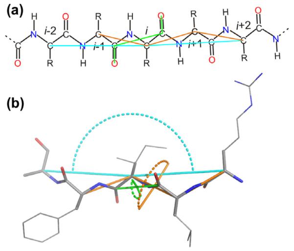
Illustration of three of the virtual angles and dihedral angles used by shAIC. (a) Schematic and (b) molecular representations highlighting the definition of the angles θ4, θ22 (see Table 2), and θ3 (see Appendix A.1), shown in green, cyan and orange, respectively, using lines through the atoms defining the angle and dotted arcs (b). Residue numbers are indicated in (a) and O and N atoms are shown in red and blue, respectively.
In the present setup, shAIC is parameterized using experimental chemical shift data extracted from a training set of 681 protein chains from high resolution X-ray and NMR structures from the refDB database [41] with less than 25% sequence identity between any pair of chains. One criterion for selecting the most appropriate model for a class is obviously that the model should provide the best agreement between observed and predicted shifts in the training set. It is natural to expect that a model with more parameters may provide a better fit, but increasing the number of parameters risks over-fitting of the data. Hence, the appropriate model is a balance between the better fit and fewer parameters. Model selection remains a highly vigorous area of research where numerous existing methods are being actively complemented with new approaches and improvements. As a consequence of the diversity in operating characteristics of model selection methods, it is necessary that the results of any specific model selection criterion be examined using an arsenal of standard diagnostic methods – for example, measure of fitness, correlation coefficient, cross validation, and ROC curves (see Section 3.3.2). A common practice is to hand-select the training data and procedures, develop the model, and then test the model using cross-validation for over-fitting. Although intuitively attractive, this approach has the risk of being inadvertently used for data subset selection and fit optimization. One way to prevent this pitfall is to incorporate model selection methods in the initial stages of the process and then use a second model selection procedure, post model fitting, to confirm that early model selection satisfies performance criteria. Methods in the family of AIC [34,35,42] and BIC [43] (Section 4.1.3) are among the better known and often-utilized methods for early model selection and they enjoy convenient relationships with cross validation. It is known that using large sample sets causes AIC to overfit the data, while BIC will underfit the same data, but the crossover point (between over and under fitting) is dependent on data. In addition, in linear models leave-one-out cross-validation is asymptotically equivalent to AIC, while leave-k-out cross-validation is asymptotically related to BIC [44–49]. Furthermore, it is well known that unbiased estimates of the generalization error based on several model selection methods do not produce consistent estimates [50]. In light of these findings, and because we do not know a priori the crossover point with respect to the number of our chemical shift sample points, we adopt a multipronged strategy. We use the AIC model selection strategy in order to maintain parsimony while we do not underfit if the sample size is in the low-medium range. To check for over-fitting, and as a second stage verification of AIC, we use leave-k-out cross-validation (leave 10% out in our cases). We further test for accuracy and sensitivity using correlation coefficient, residual errors, and ROC curves based on training data sets as well as withheld test sets. Since our subsequent leave-k-out cross validation tests do not exhibit signatures of over-fitted models, it is reasonable to suggest that AIC has produced parsimonious fittings.
Akaikes Information Criterion (AIC) [34,35,42] is an information-theoretic model selection criterion founded on minimization of the Kullback–Leibler information and likelihood inference that selects the model that fits the data best defined by the optimal balance between bias and variance. Thus, this selection criterion incorporates two properties of, fit quality, and parsimony, by selecting the model that obtains the lowest value of AIC, which is a function of the fit residual and number of parameters, by iterating over a set of models indexed by M. Accordingly, for each input geometric parameter of class, J, one optimal potential from the set of models is rigorously selected:
| (2) |
Here n is the number of data points in the training set, Pm is the number of parameters (constants) required by model m, and RSS is the residual sum of squares of the difference between observed and predicted shifts as defined in Eq. (16) (vide infra). AIC enables ranking of different models with different numbers of parameters. By including the Pm term AIC discourages over-fitting and the model with lowest AIC will have the optimal agreement between accuracy and complexity. The principle of optimal model selection using AIC is illustrated in Fig. 2 for the case of torsion angles. The residual RSS (Fig. 2b) decreases steeply with increasing model complexity (the addition of the first few knots in the spline model) and levels off at a higher number of knots. The competing contribution from the fit (represented by RSS) and the number of parameters (Pm in Eq. (2)), forces a compromise between model complexity (number of knots), and the quality of the fit – yielding a relatively more parsimonious description (see also Section 4.1 for a discussion of the consequence of using AIC for model selection).
AIC does not provide a measure to assess if a model is valid, but only enables comparison of models. Throughout the shAIC parameterization, we used a trivial “null-model”, with P0 = 0 (Eq. (2)) for comparison – using a non-trivial model only if AIC of the derived model is lower than the AIC for the trivial model. For the trivial model, , where RSS0 denotes the RSS of the training set before applying the potential. Accordingly, a geometric parameter was not used if we could not find any model m for which the following relationship would hold:
| (3) |
This procedure provides for an unbiased and optimal approach to trim the initially large set of geometric parameters in order to retain only the most relevant parameters. In addition to serving as an essential step for efficient computation, this step is significant as it encapsulates only the most important determinants of the chemical shift among short-, medium-, and long-range geometrical parameters.
shAIC utilizes the secondary structure information to capture correlations between other structural parameters that are pronounced only when the secondary structure state (helix, sheet, and coil) is known. This enables incorporation of additional and sensitive input geometric parameters, but requires the small additional cost of running the program DSSP [51] first to calculate the secondary structure.
2.3. The shAIC chemical shift force field
While shAIC is directly applicable for predicting the chemical shift, it is also straightforward to use this expression when the observed chemical shifts are known to define a force-field energy, Eshift, serving the inverse purpose, namely calculation of the structure from the observed chemical shift.
2.3.1. Definition
The shAIC chemical shift pseudo energy contribution is defined as the sum over the scaled differences for each residue, i, and atom type, n:
| (4) |
where the scaling factor, σi,n, is defined as the rmsd of the observed vs. predicted shift in the training set for each residue type in a specified secondary structure state. The final term, involving the logarithm of σi,n, prevents bias towards secondary structures with the largest scaling factors during structure calculation; an essential property since, for example, coil states have larger scaling factors relative to the other states, and hence if the logarithmic term was not used, the structure calculation would be biased towards coiled states.
2.3.2. Procedures for calculation of structural models
To test for correlation between structure and chemical shift energy, 512 structures were calculated for the protein with pdb id 1srr (one of the two proteins in the CS-ROSETTA [6] set with a solved X-ray structure) using Xplor-NIH [52]. The structures were calculated using torsion angle and distance constraints with target values measured for the reference structure (pdbID = 1SRR). In addition, the DELPHIC torsion-angle [53] and radius of gyration [54] potentials were used. Eight different structure calculations were performed, each using a different number of non-redundant randomly chosen distance restraints (including long-range), being approximately 20, 40, 80, 150, 250, 500, 1200, and 3000. Each distance restraint was chosen for short distances, d < 7 Å, between two protons, Hx(i) and Hy(j). The upper and lower bounds were set to 0.15d. For each group an ensemble of eight structures were calculated and eight such ensembles were calculated, a total of 64 structures, with different initializations of the random distance restraints. Finally, the 32 structures from each individual group (of 64 structures) having the lowest total force field and restraint energy (not shAIC energy) were kept for further analysis (i.e., the best half). The structures were calculated using a standard simulated annealing protocol heating slowly from 100 K to 3500 K while slowly ramping up the energy constants for the different types of restraints and in a second phase cooling the system slowly from the 3500 K to 100 K while slowly decreasing the restraint weights and increasing the van der Waals radii of the atoms. We note that the 1srr structure (or any homologous structure) later used for demonstration is not part of either the training set or the control set of proteins.
The shAIC chemical shift pseudo energy was calculated using Eq. (4), the rmsd in the training set between observed and predicted shift broken down into residue and secondary structure type was used as the scale constants, σi,n, and the secondary structure was calculated using the program DSSP [51]. Similar chemical shift pseudo energy calculations, using the same equation, were performed with Sparta+ predicted chemical shifts and using the same scaling constants as used for calculating the shAIC chemical shift energy. The observed correlations for this procedure are discussed in Section 4.4.1.
2.4. Definition of individual chemical shift potentials used by shAIC
During parameterization of the shAIC force field, a predefined list of potentials is provided for each input parameter class. For each class, simpler and more advanced models are provided in advance and as discussed above, the more advanced models will naturally provide a better fit but risk over-fitting which is why the optimal model from this potential list is chosen using the Akaikes information criterion (see Section 2.2). The different classes and corresponding input parameters are summarized in Table 1. For all potentials, the most basic model is the one for which the input parameter is not used, as expressed formally: . Other models are defined in detail below using the nomenclature that identifies a given atom in the residue with the index i, and secondary structure state with the index s. shAIC provides eight main classes of potentials: generalized torsion angle, side chain torsion angle, residue neighbors, secondary element length, flanking residues, ring current, packing and hydrogen bonding potentials, along with the potentials accounting for oxidation states of cysteine, cis/trans conformation of the peptide bond and an empirical correction for correlations between different chemical shifts in the same residue. The motivation for, and the impact of, choosing different models for the above physical interactions has been extensively discussed in detail previously [32,33] – therefore, this subject will not be covered exhaustively here in order to devote our major attention to the application of AIC to choose the most appropriate model among a selection of models.
2.4.1. Generalized torsion angle potentials
The conformation of the backbone torsion angles account for a large part of the variation in the chemical shift and hence it presents a key step for parameterization. A bivariate spline [32], and sums of trigonometric functions [31], have been used previously for this purpose. shAIC applies a univariate periodic cubic spline for this task: potentials for different angles, , are given by
| (5) |
where p is a univariate cubic spline polynomial [55], with m knot points, tm (not necessarily equidistant), and spline coefficients cm (a knot point is the position at which a spline changes (smoothly) from one cubic polynomial to another.) The angles θ are angles or dihedral angles from the set defined in Table 2, and they include a large set of virtual angles between atoms, not connected by bonds (see Fig. 3) – these angles offer flexibility and expandability to the model proposed by shAIC. Fig. 9 (vide infra) illustrates that the most important virtual angles as determined by shAIC have lowest AIC in relation to the experimental data. In this context, different models are splines with different number, m, of knots. In the case of dihedral angles, the spline is a periodic spline with the corresponding m + 1 spline constants giving a total of 2m + 1 parameters. Alternatively, for bend angles (normal angle defined by three points) non-periodic splines are used with the corresponding m + 4 spline constants giving a total of 2m + 4 parameters; in this case the two end-points are also used as knot points. The selection among models with respect to the number of knots is performed simultaneously with choice with respect to spline coefficients: a further option is to use specific spline constants cm = cm(R) for each different residue R or for each different neighboring residue (and the same knots for all). In this case, we would have Pm = m + 20(m + 1) = 21m + 20. The model number, and whether to use residue-specific constants, is evaluated and tested for m = 0, 1, … , 9.
Fig. 9.

Contribution, , (ppm) to the chemical shift: (a) Stacked bar plot shows the relative contribution, , from individual potentials to the predicted chemical shift (see Eq. (19)). for different atom types (horizontal axis) and secondary structures (coil/sheet/helix from left to right for each atom type). (b) Relative contribution to the chemical shift as a function of the number of fitable parameters in the model used for the potential using logarithmic axes. In both panels, the input parameters and their contributions are shown with the same color-coding scheme as in Fig. 1 (virtual torsion angles are shown in darker yellow). All values are obtained based on a training set of 681 protein chains (see text).
2.4.2. Side-chain dihedral angle potentials
The side chain adopts three main conformations for each bond free to rotate, mainly, gauche+, gauche−, and trans, which are the ranges, 0° to 120°, −120° to 0° and 120° to 180° combined with −180° to −120°, respectively. The side-chain potential, fSC(χ), encodes this information and provides a smooth interpolation between the three states using a switching function, SW(x, l, u), that maintains differentiability:
| (6) |
| (7) |
In Eq. (6) χ denotes any side chain dihedral angle χn. We note that fSC(χ) has the same form for all types of side-chain torsion angles that are free to rotate and is evaluated at a residue specific basis. This implies that fSC(χ) can be either “on” (three parameters) or “off” for a certain side-chain torsion angle in a certain residue.
2.4.3. Backbone dihedral angle potentials
This potential, fDIH(ω), for the peptide bond dihedral angle, ω, has the same expression as the above fSC potentials but with only two constants – one for the cis (−30° < ω < 30°), and one for the trans (150° < ω < 180° or −180° < ω < −150°) conformation with a switching function providing a smooth interpolation between the two states to provide differentiability as in the above.
2.4.4. Residue neighbors potentials
The nature of a neighboring amino acid has a large impact on the chemical shift, in particular for 15N. The residue neighbors potential, fRN, can also include the neighboring amino-acid side-chain conformation in the more advanced model and can, hence, be either a constant (model 1) or three constants (model 2) depending on the χ1 angle of the neighboring residue as described in the fSC potentials with a switching function interpolation between the three states.
2.4.5. Secondary element length potentials
It is desirable to include medium range information from the structure into the chemical shift prediction. This is accomplished in shAIC through incorporating the length of the secondary elements. For instance, the chemical shift is expected to be different in the middle of a helix compared to the end of the helix due to a different hydrogen bonding pattern in particular. The secondary element length (SEL) potentials, fSEL, operate on the residue type, R, of residue i and the secondary element length, Δ, which in the ± direction is defined as the smallest number, k, such that residues i and i ± k have different secondary structures (i.e. a primary-sequence “distance” to the end of the element):
| (8) |
where τR is a one-to-one look-up-table with a constant for each value of the argument, bm(Δ), and bm(Δ) is a function binning similar values of Δ together. The models differ in having a larger number of bins for more advanced models and with an advanced option to use different look-up-tables τR = τR(R) for the 20 different amino acid types, R. Some illustrative examples of results obtained from using this potential is discussed in Section 4.2.3 below.
2.4.6. Flanking residues potentials
Just as the nearest neighbor has an effect on the chemical shift, the next neighbors are important to some degree too. The flanking residues potentials, , are implemented in the same way as the nearest neighbor potentials. shAIC decided during the training phase whether a particular next neighbor is important.
The flanking residue potential, , corresponds to adding a constant to the chemical shift prediction depending on the nature of the amino acid next neighbor and of the conformation of this residue in the advanced models. To be more precise it maps a constant for each value of residue type, R, secondary structure, s, and the side chain angle canonical values (gauche+, gauche−, and trans) for χ1 (if defined) for a flanking residue with residue number, k:
| (9) |
where N is the highest residue number, τs is a look-up table mapping a constant for each different value of the secondary structure, and τm is another look-up table. In the most advanced model, τm maps a different constant for each combination of R and χ1. In this case a switching function is used to interpolate differentiability between the three different canonical values for χ1. In a simpler model, only 20 different constants are used for the different amino acids (i.e., the side chain conformation is not used). Simpler versions of these models are defined by grouping residues into seven classes of beta-branched (Ile, Val, and Thr), aromatic (Phe, Tyr, His, and Trp), amide Cγ (Asn and Gln), sulfur containing (Met and Cys), Gly, and Pro in single amino acid classes, and the rest in a common class (Ala, Ser, Asp, Glu, Lys, Arg, Leu) assigning only one constant for each group. Grouping these two options yields four different models. In the most advanced model the number of fitable parameters are: 17(20 amino acids excluding Ala, Pro and Gly having no flexible χ1 angle) · 3 + 3 (Ala, Pro and Gly) + 1(C0) + 2(the two other secondary structures) = 57. The second most advanced model as previously but grouping the residues into five groups (and Gly and Pro in separate single-member groups) yields: 5 · 3 + 3 + 2 + 1 = 23, the non-grouped model not using side-chain conformation: 20 + 2 + 1 = 23 and the most simple model grouping in the total of seven groups requires 7 + 2 + 1 = 10 parameters.
2.4.7. Oxidized/reduced Cys potential
The oxidized/reduced Cys potential, fOR, has one simple non-zero model (not depending on the structure) that assigns two different constants for Cys if it is either oxidized or reduced.
2.4.8. Ring current potentials
The point-dipole model [56], which is a function of the distance to the ring and the angle with the ring normal, offers a good approximation for the ring current effect on the chemical shift [31,57]. In order to alleviate the need for determining the best plane through the ring atoms, shAIC uses an approximation based on the standard deviation among distances from the ring atom to the sensing atom. The ring current potential, , for a certain aromatic residue, j, is defined as:
| (10) |
where std(⋃k∊jdik) denotes the sample standard deviation among distances, dik, from the given atom in residue i to a side chain carbon, k, in the aromatic residue j, denoted by the set, ⋃k∊jdik, and the sum and set is taken over all such side chain carbons in residue j. The constants, kR, Aj and Bj take three different values in the different models for this potential. In models 1 and 2, kR is kept fixed at 1. In model 1, Aj and Bj are the same two constants for all aromatic residues, j, and are different constants in models 2 and 3. In the most advanced model (model 3), kR is a different constant for each residue type, R, sensing the ring current effect. The geometric interpretation is that an atom placed directly above the ring center would have a standard deviation among the distances that is very small (σj ≈ 0) whereas an atom within the plane of the ring would have a much larger standard deviation, σj. In fact, it can be shown that for a perfectly planar ring the expression converges towards the point-dipole approximation as the number of ring atoms approaches infinity for the proper choice of constants.
2.4.9. Packing potential
The effect of solvent exposure is expected to have a high impact on the chemical shift. This effect is incorporated in the packing potential, fpack, using the sum of distances to other carbon atoms (raised to power −3 to model different degrees of packing):
| (11) |
where is the input parameter and dnk is the distance from atom n in residue i to a side chain carbon, k, in another residue j. The sums are taken over all residues separated by at least five residues from residue i. and are constants, which can be different for different secondary structure designations and different atom types. There is a choice of two models: in the simpler model and are the same constants for all different residue types, whereas in the more advanced model and are different constants for each of the 20 different possible amino acid types I of residue i. The effect of using the packing potential is discussed in Section 4.3.
2.4.10. Hydrogen bonding potentials
The effect of hydrogen bonding is modeled using the geometry of the hydrogen bond in terms of the hydrogen bond length and orientation as measured by the angle between the involved donor and acceptor atoms and either N (or Cα in case of Hα hydrogen bonding) or C’. The hydrogen bonding potentials, fHB, are the most elaborate and the model is selected from four possible models:
| (12) |
where s is a scaling factor for smooth interpolation between free and hydrogen bonded geometries:
| (13) |
| (14) |
where the input parameters are defined in the legends to Tables 1 and 2 and Fig. 4. A, B, C, D, q, ρon < 3.0, and μon, νon < cos(100π/180) are the eight free fitable parameters. ρoff = 3.0, and μoff = νoff = cos(100π/180) are fixed constants not used in the fit. In the simpler models defaults for the constants not included in the fit are used: C = 0, D = 0, q = 1, ρon = 2.7−3, νon = cos(150π/180) and μon = cos(110π/180). In model 1, only A and B are fit-able parameters. In model 2, only A, B, and C are fitted. Model 3 is the same as model 2 but with different values for A, B, and C for the different residues (60 parameters in total). In model 4, all eight constants are included in the fit.
Fig. 4.

Main parameters used for describing hydrogen bonding. Panels (a)–(e): Schematic drawing of two hydrogen-bonded β-strands showing the two angles (with double-headed arrow-arcs), θHOC and θNHO, related to hydrogen bonding of (reference atoms) HN(i), C’(i), Hα(i), C’(i + 1), and HN(i + 1). Hydrogen bonds are shown with dotted lines in the same color as the reference atom, while continuation of the backbone is indicated by broken lines. For a fixed residue, i, as shown in the second row, the other residue (the hydrogen bonding partner) being hydrogen bonded to residue i is different depending on the nature of the reference atom. This atom specific hydrogen bonding partner is indicated by “k” in panels (a)–(d). (f) and (g) show a molecular representation of two residues part of a β-bridge viewed perpendicular to (f) and parallel to (g) the hydrogen bond illustrating the angles defined in panel a for hydrogen bonding of HN as blue arcs and the virtual dihedral angle θ25 (see Appendix A) defined by the four atoms Cβ(i), Cα(i), Cα(k) and Cβ(k) shown with orange arcs (where residue k corresponds to the hydrogen bonding partner. (h) pseudo-Newman projection showing schematically the definition of ω25 indicated by an orange arrow viewing down the axis going through the two atoms Cα(i), Cα(k). (For interpretation of the references to color in this figure legend, the reader is referred to the web version of this article.)
2.4.11. Side-chain hydrogen-bonding potentials
The side-chain hydrogen-bonding potentials, fSCHB, are modeled with the same expression but fewer fitable parameters compared to the main-chain hydrogen-bonding potential. The potential, fSCHB, has one non-zero-model. For n = Hα or n = HN a special potential for hydrogen bonding of this proton with a side-chain acceptor atom in Asn, Asp, Glu, Gln, Ser, or Thr is tested. The same expression as for the main-chain hydrogen bonding is used with defaults A = 0, D = 0, q = 1, ρoff = 3.0, μoff = νoff = cos(100π/180), μon = νon = cos(200π/180). B and ρoff < 3.0 are free parameters allowing two different values for B for the carbonyl acceptor class with residues Asn, Asp, Glu, Gln and sp3 acceptor class oxygen of Ser and Thr. C = 0 is used for the Ser and Thr case, whereas C is a free parameter for the carbonyl acceptor class giving a total of four free parameters.
2.4.12. Correction term for other chemical shift effects
The chemical shift will also be affected by factors other than the structure or the primary sequence; for example, referencing errors, buffer conditions local mobility and isotope effects. It is expected that such factors will be correlated among the chemical shifts of nearby atoms. Hence, a correction term, in Eq. (1), is applied to correct empirically for such factors. The constant is dependent on the chemical shifts for the nuclei near n in residue i, defined as:
| (15) |
where the index set k ∊ N denotes all backbone and Cβ and Hβ atoms close to n which are the atom in the same and the neighboring residues, and denotes the observed and average chemical shift, respectively, of atom k and the average is for atoms of the same residue type, I, and secondary structure and ak,R (which can be zero indicating that the corresponding atom is not used) are the fit-able atom specific constants. AIC is used, analogous to the fitting of the potentials, to determine if the constants should be zero, common for all residues or residue type specific if the advanced model is chosen.
2.5. Protein structure datasets
The refDB database [41] (from January 2008) was downloaded and used as the starting point for the derivation of the dataset, yielding a set of 1565 protein chains from protein structures determined by X-ray crystallography or NMR and their corresponding uniformly referenced chemical shifts. Of this set 1063 were selected having a resolution of, R < 2.5 Å for X-ray structures. For NMR structures, the rmsd between the representative model and the other models of the ensemble was required to be <2.5 Å for a heavy atom best fit of either all residues or all residues in helices, sheet or turns which were defined as the E, H, or T records calculated by DSSP [51]. Note that our enforcement of this requirement for the NMR structure does not imply that NMR structures have a comparable accuracy to an X-ray structure with an rmsd of 2.5 Å. This set was further filtered using the PDB_SELECT algorithm [58] selecting chains having <25% sequence identity using a customizing quality function ensuring that the chains with highest quality and with the most assigned chemical shifts were kept. This final filtering yielded the set designated as St, which is a set comprised of 681 chains of which 233 are from high-resolution X-ray structures. The bmrIDs and pdbIDs for all these chains are provided in the Tables A2 and A3 in Appendix A. The X-ray structures were protonated using the program reduce [59], the secondary structure was determined by the DSSP program [51]. Here “E” records are referred to as sheet states, the “H” and “G” (alpha-helix and 3-helix, respectively) records as helix states and the rest of the records as coil states. Distances and torsion angles in the protein were measured using the programs MMLIB [60] or BioPython [61]. For X-ray structures, crystal contacts and true oligomeric contacts were differentiated using the program PISA [62] and by visual inspection.
A control set of structures was derived using the same procedure as above but this time using the refDB database as of August 2009 comprising 2115 entries and keeping only the X-ray structures having a resolution R < 2.5 Å. By using PDB_SELECT [58] all chains with >25% sequence identity with any chain in the set St and among chains within this new set were removed yielding a control set Sc of 38 chains. Since the Sparta+ machine learning approach had the best performance among existing software, two subsets were derived from Sc for test purposes. One subset consisted of chains that have less than 25% identity to either training set – shAIC or Sparta+. The second set focused on selecting a subset from the 38 chains that have an NMR structure corresponding to the X-ray structure. Sequence alignment was carried out using the pdbSelect procedure [58]. The matching between NMR structure and the corresponding X-ray structure was accomplished using the BMRB website. The bmrIDs and pdbIDs for all these chains are provided in Table A1 in Appendix A.
2.6. Parametrization of shAIC
Prior to applying shAIC to predict the chemical shift of an unknown protein, the set of parameters that define the shAIC chemical shift predictor need to be determined. Once the constants, cj,n,s, and potentials, fj, are known, then Eq. (1) is applied for each backbone atom after calculating the geometric parameters. In order to determine the unknown parameters of our model, the derived database of 681 protein chains with their corresponding assigned chemical shift (the training set) was used to obtain an optimal fit for constants and the potential functions for each j, n, and s.
The parameterization was accomplished in an iterative process grouping all nucleus and secondary structure types as a data set and fitting each different class, J, sequentially through four cycles. Each input parameter k = J was fitted separately for all possible models, m, keeping the other potentials and constants for j ≠ k fixed using:
| (16) |
where the chemical shift residual, Δδi,n,k is the difference between the observed chemical shift and the chemical shift calculated without contribution from the potential, k:
| (17) |
and fj = 0 was used in the first iteration for all potentials that were not yet fitted.
Potential AIC-based model-selection bias toward normally distributed data can lead to tendencies towards selecting the models with most parameters – particularly if outliers are present or if the data is over-dispersed in general [42]. This scenario is properly dealt with using the following procedure: at each step of the iterative process, all data points with
| (18) |
where ⟨Δδi,n,k⟩s denotes the sample standard deviation of Δδi,n,k among all the data with same secondary structure, are not included in the fit for T = T0 (ca. 2% of the data points) and removed completely from the database. The value of T0 was systematically varied. At T0 = 5 ~0.5% to 1% of the data points were removed, while at T0 = 3 approximately 2% of the data points were removed. Varying T0 between 2 and 4 had little impact on the accuracy of shAIC as judged by the performance on the 38 chains test set, with T = 3 being the value yielding the lowest rmsds and, hence, this value is used consistently throughout. Outlier residues are removed using a criterion similar to that above with respect to the sum of the squared errors of the shift residuals within the residue. The threshold is computed dependent on the number of assigned chemical shifts in the residue using a transformation from the chi-squared distribution to a normal distribution [63] and using T = 5 as in the above.
Potentials are fitted using either closed analytical expressions, or a least squares fit applying a Levenberg–Marquardt algorithm [64,65] or a more advanced method (used for the non-linear model for the hydrogen bonding contribution); the Nelder–Mead down-hill simplex algorithm [66]. The torsion angle contribution is fitted using a combination of a spline fitting [67] and a simulated annealing procedure provided through the python scientific computing package [68]. All calculations were performed on a Pentium 4 Linux workstation equipped with 2 cores with 3 GHz processors, or on an AMD/Opteron computer cluster using eight parallel 2.3 GHz processors.
3. Performance of shAIC chemical shift prediction
In this section, the performance of shAIC for prediction of protein chemical shifts is evaluated and compared to existing methods. In addition to relative measures on chemical shifts, the results also address the capability of shAIC to include longer-range interactions in the prioritized parameterization. This may shed interesting new light on important experimental measurements as well as structural determinants. The results outlined here will be discussed in more detail in Section 4.
3.1. Criteria used to evaluate the performance of shAIC
The performance of shAIC was evaluated based on tests that stress accuracy, precision, and robustness i.e. the ability to generalize beyond the training set. The multifaceted procedure used to test shAIC provides substantial and detailed information regarding its performance characteristics on several methodically selected subsets that highlight the challenges in chemical shift prediction. Other relevant properties of shAIC such as smoothness, explanatory power, and speed of computation are dealt with in Section 4. The accuracy and precision of shAIC is tested relative to state-of-the-art methods using several detailed performance measures that include NMR and X-ray structure subsets in order to identify performance characteristics that are otherwise difficult to discern. The generalized performance of shAIC is measured using a “held-out” test set as well as a cross-validation procedure as a measure of the robustness of the method aiming to justify that shAIC is applicable not just to certain special cases of structures. The tests include a partial-area-under-curve measure that identifies accuracy-performance trade-offs for other approaches along-side shAIC and performance analysis on different ranges of chemical shifts and robustness in the dependence on secondary structure.
3.2. Absolute performance of shAIC
In this section we analyze the absolute performance of shAIC using different quality parameters and validation techniques. Performance in specific cases within shAIC is compared whereas comparison to other methods are described in Sections 3.3 and 3.4.
3.2.1. Performance on the “held-out” set
A control set of 38 protein chains from high-resolution X-ray structures was constructed (see Section 2.4) with less than 25% sequence identity to any chain within the training set (used to parameterize shAIC) and within this control set. This set was used for the evaluation of the rmsd between observed and predicted chemical shifts (Table 3 part B). We also evaluated the square of the Pearson correlation coefficient (coefficient of determination), R2, for predicted vs. observed chemical shifts in this set. Since different amino acids have markedly different average chemical shifts, it is relevant to analyze the correlation for observed vs. predicted secondary chemical shifts, i.e., the shift minus the average chemical shift, for the specified atom and residue type. Furthermore, we analyzed the correlation for the tertiary chemical shift, i.e., for vs. where and are the predicted and observed chemical shifts, respectively, and is the average chemical shift in the training set of the particular atom type, residue type, and secondary structure. This refinement uses the already known secondary-structure states in order to gain more detailed insight into the dependence of prediction performance on structural state. This definition makes the statistical comparison among different nuclei more meaningful. Henceforth in this section, R2 will be reported for the tertiary chemical shift. As would be expected, R2 for secondary, and more so for tertiary chemical shifts, is lower when it is compared to the same values for the “uncorrected” chemical shifts. The mean R2 (tertiary chemical shift) for shAIC is 0.53 averaged over all atoms – with the highest values for 15N (0.653), implying that the 15N chemical shift offers most information on the structure in cases where the secondary structure is considered known. The high information content for 15N is notable since 15N is often regarded as the most difficult chemical shift to predict. It is also observed that shAIC shows the highest correlation in regions identified as sheet secondary structures, while it demonstrates lower correlations for helices and coil states. This is probably because the high variation in the structure of β-sheets compared to helixes. The relatively low correlation in the coil states despite the larger variation in structure is probably due to more disorder in these states.
Table 3.
Performance of shAIC relative to other methods evaluated using the control set of 38 proteins and cross-validation of shAIC.
| Part A. Comparison with existing programs |
Part B. shAIC: overall and segregated |
||||||||
|---|---|---|---|---|---|---|---|---|---|
| ShiftX | Sparta | CamShift | SHIFTS | Sparta+ | ShAIC | Sheet | Helix | Coil | |
| Correlation coefficient squared, Rtert2, for tertiary chemical shift a | |||||||||
| N | 0.520 | 0.564 | 0.468 | 0.282 | 0.661 | 0.653 | 0.721 | 0.600 | 0.653 |
| C’ | 0.243 | 0.370 | 0.336 | 0.089 | 0.478 | 0.462 | 0.528 | 0.476 | 0.382 |
| Cα | 0.443 | 0.522 | 0.395 | 0.328 | 0.621 | 0.594 | 0.577 | 0.621 | 0.602 |
| Cβ | 0.350 | 0.455 | 0.399 | 0.172 | 0.533 | 0.477 | 0.573 | 0.396 | 0.479 |
| HN | 0.370 | 0.389 | 0.405 | 0.172 | 0.523 | 0.451 | 0.521 | 0.468 | 0.437 |
| Hα | 0.533 | 0.475 | 0.548 | 0.422 | 0.614 | 0.543 | 0.573 | 0.447 | 0.450 |
| Correlation coefficient squared, Rsec2, for secondary chemical shift a | |||||||||
| N | 0.577 | 0.616 | 0.531 | 0.333 | 0.701 | 0.694 | |||
| C’ | 0.555 | 0.643 | 0.624 | 0.340 | 0.704 | 0.696 | |||
| Cα | 0.741 | 0.784 | 0.724 | 0.661 | 0.828 | 0.815 | |||
| Cβ | 0.556 | 0.632 | 0.591 | 0.381 | 0.687 | 0.649 | |||
| HN | 0.435 | 0.455 | 0.463 | 0.249 | 0.573 | 0.508 | |||
| Hα | 0.721 | 0.695 | 0.733 | 0.647 | 0.772 | 0.733 | |||
| Rmsd/ppm (control set) | Rmsd/ppm shAIC (training set) | |||||||
|---|---|---|---|---|---|---|---|---|
| Derivationb | Cross-validationc | |||||||
| N | 2.827 | 2.694 | 2.905 | 4.313 | 2.356 | 2.343 | 2.391 | 2.561 |
| C’ | 1.253 | 1.105 | 1.128 | 1.756 | 1.004 | 1.016 | 1.074 | 1.172 |
| Cα | 1.144 | 1.044 | 1.175 | 1.337 | 0.926 | 0.961 | 0.946 | 1.035 |
| Cβ | 1.219 | 1.099 | 1.157 | 1.525 | 1.012 | 1.071 | 1.138 | 1.336 |
| HN | 0.559 | 0.546 | 0.528 | 0.630 | 0.466 | 0.503 | 0.465 | 0.501 |
| Hα | 0.283 | 0.318 | 0.276 | 0.319 | 0.262 | 0.276 | 0.262 | 0.280 |
| 90% confidence intervals d /ppm (control set) | ||||||||
| N | 4.476 | 4360 | 4.674 | 7.005 | 3.675 | 3.769 | ||
| C’ | 1.988 | 1.749 | 1.838 | 2.841 | 1.631 | 1.626 | ||
| Cα | 1.822 | 1.639 | 1.896 | 2.153 | 1.409 | 1.462 | ||
| Cβ | 1.993 | 1.761 | 1.865 | 2.425 | 1.651 | 1.750 | ||
| HN | 0.884 | 0.872 | 0.827 | 0.958 | 0.725 | 0.798 | ||
| Hα | 0.451 | 0.528 | 0.454 | 0.520 | 0.393 | 0.421 | ||
Squared correlation coefficients (coefficient of determination) for observed vs. predicted tertiary or secondary chemical shift is described in the text. Only chemical shift values for which all programs provided a prediction were included in the analysis (e.g., Sparta does not provide predictions for terminal residues). Outliers were removed from the analysis based on the criteria that, for all methods, the error was larger than five times the standard deviation, with the standard deviation estimated from rmsds in the training set broken down into residue and secondary structure type.
rmsds between predicted and observed chemical shift in the training set of 681 proteins after derivation of all parameters.
rmsds between predicted and observed chemical shift in the training set of 681 proteins using cross-validation. The set was divided into 10 equal subsets and for each subset the 9 other sets were used to derive the parameters, which in turn was used to predict the shift for the first set.
90% of the predictions have an error less than this threshold.
3.2.2. Cross-validation
We also performed a cross-validation test to further substantiate the shAIC method by splitting the 681 training set into 10 equal parts and for each set only using the other nine sets to derive shAIC used for the prediction (see Section 2). The rmsds (for all cases of atom types and secondary structure classes) for the unified left-out sets between observed and predicted chemical shifts is on a par with the rmsds obtained by using the control set. Because the control set contains only X-ray structures, whereas the training set contains both X-ray structures and NMR structures, small deviations are likely and are reasonably attributable to the differences in the control and training sets. In practice, taking into consideration the approach taken by shAIC for the selection of minimal training data set, and the active selection of the smallest parameter set, the slight increase in rmsds in 10-fold cross-validation by ca. 10% is expected (see Table 3, part B). A more detailed discussion is provided in Section 4.1.3.
3.2.3. Analysis of residuals
Analysis of the variations in the errors is useful for diagnosing problems and identifying regions for further improvement. We measure the error in the prediction (residual) as a function of the true secondary chemical shift and examined the results for bias in distribution in any region. Our observations suggest that the errors are relatively even across the range of shifts (see Fig. 5). However, as would be expected, for extreme chemical shifts (those typically beyond three standard deviations of the mean), the observed errors show bias. In other words, a certain nuclei having very low value for the chemical shift typically over-estimate the chemical shift in the prediction and vice versa (this dependence was similar for Sparta+). Our results therefore suggest that shAIC will be useful for chemical shift prediction in most cases.
Fig. 5.

The residual error, Δδ, which is the difference between the observed and predicted chemical shift, shown as a function of the observed secondary chemical shift for the six different atom types. The lines y = x (full line) and y = 0 (dotted line) are shown for reference.
3.2.4. Dependence on secondary structure classification
shAIC uses the secondary structure to switch between the parameter sets related to different secondary structures. This requires the secondary structure to be determined before running shAIC and this can be accomplished quickly by running DSSP [51]. When using shAIC as part of a structure calculation, the secondary structure should be updated at regular intervals using a definition similar to DSSP. It can be argued that “misclassifying” the secondary structure would lead to errors or, put in another way, a residue at the ends of, e.g., a helix would be “in between” a coil and an α helix and that the predicted chemical shift would depend irregularly on the classification. To analyze this scenario, the residues in the evaluation set of 38 proteins found at the ends of the secondary elements were misclassified to a coil residue. The rmsds between predicted and observed chemical shifts for these residues increased only slightly, ca. 10% on average (see Fig. 6), indicating that shAIC is robust with respect to the mis-assignment of the secondary structure at positions on the border between coil and structured state. The largest difference is observed for helixes for Cα and Cβ. This is not surprising since the chemical shift for these atoms vary considerably with the secondary structure. From an opposite point of view, this dependence on the secondary structure classification (albeit weak) would help in determining the secondary structure by minimizing the shift energy (Eq. (8)) during structure calculation (Section 4.4). It should be noted that shAIC does not require that the secondary structure determined by DSSP before chemical shift prediction is the “true” secondary structure in reference to some universal state, because the DSSP determined secondary structure is only used as a means to expand the parameter set.
Fig. 6.
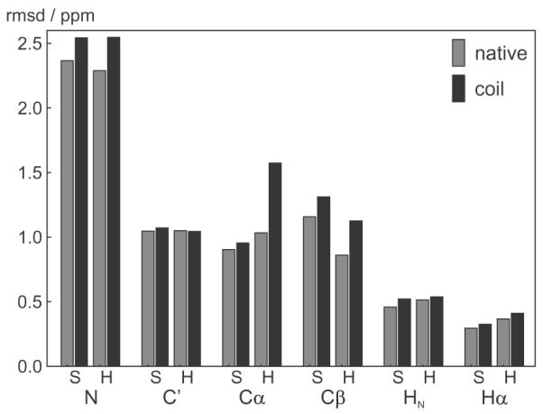
rmsds between observed and predicted chemical shift for native and mis-classified secondary structures. The bars show the rmsd in the evaluation set of 39 protein chains for the residues at the end of the helixes (H) and sheets (S) using the correctly assigned secondary structure (gray) and using a state mis-classified to a coil residue (black), hence using the native and the coil shAIC parameters, respectively, to calculate the predicted shift.
3.3. Performance of shAIC relative to previous methods
To evaluate shAIC and obtain comparative measures among different methods, we performed a side-by-side comparison with other state-of-the-art methods: SHIFTX [32], CamShift [31], SHIFTS [20], Sparta [33], and Sparta+ [23].
3.3.1. Performance on the “held-out” set
First the correlation between observed and predicted chemical shift for a 38 chain “held-out” set (Section 2.5) was compared for the different methods. It should be noted that this set does not contain any chain with >25% sequence identity to any chain in the set used for training shAIC, but in contrast we chose not to remove the chains having >25% sequence identity to a chain in sets used for training the other methods in order to preserve a reasonable size to provide a sound statistical basis for comparing the rmsds. It is expected, although difficult to quantify, that this higher homology to their training sets for the other methods would have a favorable impact on the performances of the other methods. Despite this fact, as illustrated in Fig. 7a (Table 1, part A), we found that the rmsds for shAIC for this set evaluation set are yet significantly better than all other methods with some exceptions for Sparta+. Although Sparta+ uses a machine-learning approach, that strictly speaking is considered a “black-box” approach, we found it informative to include the comparisons. The ratios between the rmsds for this particular test-set for shAIC and Sparta+ ranged from 7% lower rmsd for Sparta+ in case of HN, to a negligibly lower rmsd for shAIC in case of N. The program SHIFTS, a hybrid approach, performed considerably less favorably when compared to the other methods. Among these methods, CamShift [31] is also reported to have a differentiable formulation for its empirical prediction. Comparison of results from shAIC and CamShift revealed the largest rmsd difference for the Cα chemical shift – for which the rmsd is 0.961 ppm for shAIC and 1.175 ppm for CamShift. For heavy atoms, the performance of shAIC was noticeably superior to CamShift. A more elaborate and rigorous comparison between shAIC and Sparta+ is performed below (see Section 3.4).
Fig. 7.

rmsds between observed and predicted tertiary chemical shift for different test sets (see Section 2) comparing the performance of shAIC and previous methods (see coding for bar filling in legends). (a) A control set of 38 protein chains having less than 25% sequence identity to any chain used to train shAIC, (b) a subset of 8 out the 38 chains having less than 25% sequence identity to the chains used for training Sparta+, (c) the set used for evaluating CS-ROSETTA after removing all chains already present in the shAIC training set, (d) a set of 19 chains consisting of the NMR ensembles for the entries in the 38 protein chain set in panel (a), for which NMR structures were available. The rmsd for the NMR ensemble was calculated by evaluating differences between observed chemical shift and the average of the predicted chemical shift for all members of the ensemble (designated by “ens” in the legend) and by evaluating the difference prior to evaluating the average (designated by “ave” in the legend). The insert in (d) shows the standard deviation within the ensemble averaged over all residues, s, for Hα shown as a blue dot for each protein in the set Sparta+ as a function of the corresponding value for shAIC with the identity line x = x as a dashed line shown for reference. (For interpretation of the references to color in this figure legend, the reader is referred to the web version of this article.)
3.3.2. False positive rate analysis
Central to the task of constructing predictive models is the question of model performance assessment [69]. Some traditional performance metrics have been shown to be sensitive to the choice of training data [70] – for example in neural network models [71]. Receiver Operating Characteristic (ROC) curves, which plot true positive rates against false positives, visually convey useful information in an intuitive and robust fashion [72]. Using the 38 chains in the “held-out” set, we examined the fraction of predictions outside of the threshold (false positives) as a function of error threshold. A striking aspect of ShAIC’s performance is that it attains a consistently higher true positive rate at every threshold (excluding endpoints) than the other methods, and a similar or slightly lower rate compared to Sparta+ (see Fig. 8). This data suggests that shAIC peforms better over a broad range – i.e. that its better average performance is across the board and is not limited to a specific subset of the data.
Fig. 8.

The fraction of assignment errors, ferr (Terr) as a function of the error threshold, Terr. Each point in the plots represents a threshold, Terr, and the corresponding fraction of predictions, ferr, having an error larger than this threshold. The plots were derived from the 38-chain validation set. shAIC (blue lines) are compared with other methods for all six atom types. Note the logarithmic y axis. (For interpretation of the references to color in this figure legend, the reader is referred to the web version of this article.)
3.4. In depth and rigorous comparison between shAIC and Sparta+
The above analysis provides a survey of the performance of different methods relative to shAIC. However, a more detailed analysis should consider the differences in overlap between training and test sets in the various approaches. Since the performance of Sparta+ was the closest relative to shAIC, we selected Sparta+ as a basis for a more detailed comparison to shAIC in order to gain new valuable insights.
3.4.1. Performance on proteins distantly related to the training sets
In order to provide a more rigorous comparison between the two powerful methods the comparison was repeated on a subset of the “held out” set used for evaluation described above. A new subset having less than 25% sequence identity to any chain in the set used for training Sparta+ was formed for further testing. Hence, we removed 30 out of the 38 chains and retained the subset of 8 out the 38 chains (see Table A1 in Appendix A) for further investigation. In this more appropriate comparison the overall performance of shAIC was marginally better than Sparta+ (c.f. Fig. 7b). These results suggest a subset dependence of generalization error for both Sparta+ and shAIC. However, the apparently smaller generalization error found for shAIC might indicate a marginally better performance of shAIC (on average) for a novel structure having no high sequence identity to any protein chain in the set used for training shAIC and Sparta+. A practical implication of this observation may be that in cases where a homologous protein is available, standard structure prediction tools without the need for experimentally determined chemical shifts could be used to predict the structure. In cases where no homologous protein is at hand, a powerful method for predicting the chemical shift remains highly valuable.
3.4.2. Performance on NMR determined structures
We also investigated the relative performance characteristics of shAIC vs. Sparta+ on NMR subsets to discern if there is a measurable performance difference between shAIC and Sparta+ on structures determined by NMR. I.e. we specialized the subset of 38 protein chains to those for which an NMR-derived ensemble of structures was available leading to a subset of 18 structures and we compared the rmsds between observed and predicted shifts for this subset (c.f. Fig. 7d). The rmsds for the structures derived by X-ray in this set had the same trends as the full set. However, when the corresponding NMR structures were used as the basis, the results show a significantly better rmsd for shAIC compared to Sparta+ for all nuclei (the results held irrespective of rmsd being evaluated before or after averaging the predicted shift within the ensemble). This suggests that shAIC would be an ideal approach to aid structure determination by NMR as will be illustrated with examples in Section 4.4.
3.4.3. Performance of shAIC on NMR subsets previously used for chemical-shift-based structure determination
NMR chemical shifts have been used to determine structure without the aid of long-range contact information. The successful structure determination results (for example, in the data set used for experiments with CS-ROSETTA [6]) suggest that in this data set there is a strong and demonstrably robust relationship between chemical shifts and structure information. Therefore, it was expected that this robust relationship would hold also in the direction of structure to chemical shifts. The performance of shAIC and Sparta+ was evaluated by using the set used for CS-ROSETTA [6] evaluations after removing all chains already present in the shAIC training set (c.f. Fig. 7c). The resulting rmsd values confirmed the earlier conclusion that shAIC performs significantly better when predictions are based on NMR structures (all structures within this set except two are NMR structures). Next, it was relevant to investigate the relationship in the scatter of predicted chemical shifts as a result of geometric scatter in the NMR ensemble. Scatter in the predicted chemical shift values for the same atom within the ensemble is smaller in the results reported by shAIC as compared to Sparta+, which provides an important reporter for robustness (c.f. Fig. 7d, insert). The higher precision may be suggestive for the selection of the “best model” among conformers in an NMR-derived ensemble, which is discussed in Section 4.4.1.
4. Discussion of merits: explanatory power, chemical shift prediction, and structure calculation
Models proposed for chemical shift prediction have the potential to be useful and informative beyond their original purpose. Using the results in Section 3, we discuss here the analytical model used by shAIC in the context of existing methods. In addition to applications of chemical shift prediction, which is the focus here, we aim at two other important areas: (a) explanatory power in providing physical insight into protein structure and (b) structure determination. Although, as mentioned, the latter is not our primary aim in the present work, its importance as a direct application of chemical shift modeling merits discussion.
4.1. Impact of regularized model selection with AIC
While some existing methods use post-optimization validation tools to evaluate their model selection criteria, shAIC utilizes the statistical regularization approach of AIC as a theoretical basis for optimal parameter set selection. The impact of using AIC is analyzed here using illustrative examples and comparisons.
4.1.1. Correspondence between the number of parameters and the contribution to the chemical shift
The attempt by AIC to avoid unsupported assumptions on the model is evident in trends whereby potentials having the largest contribution to the chemical shift (see Eq. (19) below and Fig. 9b) are parameterized with the largest number of parameters and vice versa as discussed with examples below. The relative contribution to the chemical shift, , for a specific nucleus and secondary structure to the chemical shift from a certain class, J, of input parameters may be described as:
| (19) |
where is the observed chemical shift; the remainder of the variables are defined in Eq. (1). For example, the torsion-angle potential, which has the largest contribution to the chemical shift, is parameterized using the largest number of parameters (see also Table 4). Conversely, the long-range effects, packing and ring current, have the smallest impact on the chemical shift and are also parameterized with the smallest number of parameters. In addition, within the same class nuclei experiencing the largest impact from the potential corresponding to that particular class are also parameterized with the largest number of parameters (see Table 4).
Table 4.
Number of parameters and contribution to the chemical shift (shown in parenthesis as defined in Eq. (19)) for each potential in columns 4–11 (showing the class number below the potential name, as defined in Table 1), atom type (col. 1) and secondary structure, s, (col. 2; S, H, and C referring to β sheet, helix and coil states, respectively). The total number of chemical shifts, tot, used for training shAIC for each combination of atom type and secondary structure is shown column 3.
| Atom | s | Tot | Hbonding J = 5 |
SEL J = 8 |
flankRes J = 7 |
Neighbors J = 4 |
Packing J = 10 |
Ring Current J = 9 |
Side chain J = 2 |
Torsions J = 1 |
|---|---|---|---|---|---|---|---|---|---|---|
| C’ | C | 15,863 | 18(0.101) | 17(0.034) | 53(0.094) | 78(0.250) | 20(0.105) | 8(0.059) | 46(0.101) | 725(0.464) |
| C’ | H | 13,333 | 3(0.027) | 18(0.207) | 203(0.219) | 66(0.166) | 20(0.085) | 2(0.102) | 42(0.095) | 281(0.369) |
| C’ | S | 9920 | 19(0.175) | 10(0.126) | 122(0.175) | 80(0.221) | 20(0.088) | 8(0.070) | 62(0.214) | 330(0.399) |
| Cα | C | 23,224 | 3(0.025) | 0(0.000) | 43(0.049) | 72(0.352) | 20(0.041) | 8(0.045) | 66(0.139) | 1543(0.617) |
| Cα | H | 17,961 | 5(0.096) | 320(0.336) | 130(0.142) | 56(0.128) | 20(0.095) | 8(0.062) | 66(0.192) | 596(0.412) |
| Cα | S | 13,222 | 17(0.129) | 11(0.048) | 66(0.094) | 70(0.209) | 20(0.071) | 2(0.057) | 52(0.266) | 670(0.528) |
| Cβ | C | 18,631 | 11(0.037) | 152(0.122) | 41(0.069) | 72(0.082) | 19(0.089) | 8(0.086) | 58(0.113) | 1168(0.557) |
| Cβ | H | 16,100 | 12(0.049) | 285(0.209) | 51(0.085) | 53(0.164) | 19(0.069) | 8(0.086) | 48(0.142) | 166(0.216) |
| Cβ | S | 11,733 | 48(0.108) | 12(0.054) | 20(0.045) | 86(0.130) | 19(0.105) | 26(0.111) | 46(0.178) | 690(0.558) |
| HN | C | 26,030 | 11(0.143) | 0(0.000) | 97(0.157) | 90(0.138) | 19(0.042) | 26(0.116) | 34(0.071) | 611(0.444) |
| HN | H | 20,311 | 14(0.146) | 274(0.275) | 200(0.186) | 86(0.168) | 19(0.049) | 8(0.122) | 36(0.079) | 475(0.327) |
| HN | S | 15,051 | 21(0.230) | 7(0.129) | 181(0.192) | 94(0.242) | 2(0.048) | 26(0.107) | 34(0.075) | 434(0.431) |
| Hα | C | 24,437 | 20(0.184) | 6(0.052) | 20(0.047) | 76(0.207) | 20(0.037) | 27(0.180) | 44(0.103) | 756(0.433) |
| Hα | H | 17,447 | 11(0.113) | 9(0.115) | 169(0.202) | 84(0.205) | 20(0.165) | 8(0.217) | 46(0.141) | 382(0.268) |
| Hα | S | 12,894 | 7(0.223) | 0(0.000) | 161(0.198) | 86(0.141) | 2(0.102) | 8(0.207) | 48(0.137) | 449(0.488) |
| N | C | 22,170 | 0(0.000) | 0(0.000) | 51(0.095) | 86(0.335) | 2(0.055) | 8(0.021) | 58(0.164) | 1136(0.585) |
| N | H | 18,189 | 14(0.079) | 166(0.222) | 189(0.224) | 92(0.325) | 2(0.053) | 8(0.058) | 58(0.197) | 661(0.426) |
| N | S | 13,644 | 12(0.042) | 7(0.167) | 139(0.137) | 96(0.467) | 2(0.079) | 8(0.027) | 56(0.289) | 421(0.451) |
4.1.2. Justification of using AIC compared to conventional approaches
The advantage of using AIC as the optimization criterion may be quantitatively evaluated by considering two other criteria: the minimal fit residual (RSS), which is commonly used, and the minimal number of parameters (see Fig. 10). Using the RSS approach exclusively (i.e., minimizing the difference between observed and predicted shifts), 2–3 times more parameters (depending on the specific case) were selected. This inclusion of more parameters leads to a better fit for the training data. However, in this case, the empirical functions with a larger number of parameters yield an R2 for the control set that is approximately 5% lower (corresponding to a higher RSS) when compared to using AIC – suggesting possible over-fitting of the training data. Conversely, when using the model with the minimal number of parameters (pushing it the most to avoid over-fitting), many fewer parameters are included and the RSS of training is the lowest of the three cases, but the RSS of the control set used for evaluation also decreases again approximately by 5%, suggesting a case of under-fitting. Applying AIC to choose the optimal potential leads to a number of parameters in-between the two other cases and yields the better RSS of the control as a result of the balanced fitting.
Fig. 10.
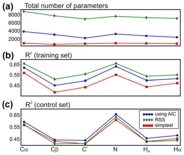
Evaluation of different optimization methods, showing (a) the number of parameters used in all the potentials in total, (b) the R2 in the training set (calculated as 1-RSS/RSS0, where RSS and RSS0 is the RSS calculated without and with using the shAIC potential, respectively) R2 after parameterization and (c) R2 in the control set. Properties are shown for calculations using AIC (blue circles), RSS (green diamonds) and choosing always the simplest model (red squares) as the minimization criterion. (For interpretation of the references to color in this figure legend, the reader is referred to the web version of this article.)
4.1.3. Comparison to other information criteria
To be more quantitative we have performed an analysis where the number of parameters was gradually increased to observe the effect on the predictive power. Another version of AIC (the quasi AIC, qAIC) is defined by scaling the fit residual part of AIC with the variance inflation factor, ĉ:
| (20) |
A high value of ĉ indicates that because of correlation within the data the variance is higher than it would be if the data were totally uncorrelated. The corrected formulation of AIC states that in such cases the weight used for the fit quality (RSS) should be downscaled. However, ĉ is not known a priori and very difficult to estimate, but for the case of protein structure data it would be reasonable to suggest that its deviation from unity is small. The expression for qAIC can be rewritten for cases where only ranking of models is intended:
| (21) |
where c(n) is the constant, ĉ, in the case of qAIC. Other information criteria exist for ranking models. Thus, the Scwartz criterion, also called the Bayesian Information Criterion (BIC) [43], can be written in the above form with c(n) = ln(n)/2, and is also used widely and penalizes parameters harder than AIC but also risks under-fitting. The Hannan–Quinn information criterion (HQC) [73] uses c(n) = ln(ln(n)) and penalizes the number of parameters harder than AIC but less than BIC for n in the ranges used in this analysis.
A systematic analysis was performed comparing different information criteria by using corrICm for different values of c(n) = ĉ for model selection during training (with ĉ = 1 corresponding to the generic AIC). This analysis was performed for three representative cases, Cα in the coil state, Cβ in helixes, and N in sheets comparing the total number of parameters used and rmsd between observed and predicted shifts in the training set (training rmsd) and the control set (evaluation rmsd) having 39 protein chains with low similarity to the training set. Note that the difference between the two datasets and the different procedures for determining outliers in the sets causes differences in the rmsd when comparing the two sets (see legends to Fig. 11 and Table 3). This difference is particularly large for Cα, however, it is still possible to analyze the impact of a systematic variation in the information criteria, since the initial slopes at high values of ĉ are comparable and hence, extrapolation is possible. It is observed (reading the charts in Fig. 11 from right to left) that increasing the number of parameters (exponentially) as accomplished by varying ĉ leads, naturally, to a (linear) decrease in the training rmsd. For low values of P, the trend in training rmsd is mirrored in the evaluation rmsd. However, at some point starting between ĉ = 2 and ĉ = 5, the evaluation rmsd start decrease with lower rate compared to the training rmsd; at this point over-fitting starts to deteriorate the quality of the prediction. At the other extreme for ĉ < 1 over-fitting causes the evaluation rmsd to increase rapidly. Finally, at values between ĉ = 1 and ĉ = 2 the evaluation rmsd reaches its lowest value corresponding to the points where the gain by using more parameters equals the accepted costs of over-fitting the data. For the three cases studied here we have for BIC: c(n) = 4.84, 5.03, 4.76 for Cβ, Cα and N, respectively. Furthermore, for HQC: c(n) = 2.27, 2.31, and 2.25. We conclude following our analysis, as judged by the evaluation rmsd, that BIC produced a parameter set with inferior predictive power compared to when using AIC. Conversely, the less frequently used HQC leads to a similar performance compared to AIC. In general, the optimal performance is observed for values between ĉ = 1 and ĉ = 2. Applying this corrected model selection criteria leads to a decrease in the evaluation rmsd of ca. 1%. We argue that using the generic AIC (ĉ = 1) can be justified since the gain in performance is very small for choosing a non-unity ĉ.
Fig. 11.

Analysis of the impact of variation in model selection criteria on the predictive power of shAIC. Variations are observed as a function of the variance inflation factor (Eq. (20)), ĉ. For each value of this parameter the shAIC parameter set was fitted to the training data using Eq. (21) as the model selection criteria following procedures described here for the generic case. The number of parameters, P, is the total used in the full parameter set. The training rmsd was evaluated as that between observed and predicted shifts in the training set using only the X-ray part of the training set in order to provide a set more similar to the evaluation set and removing outliers judged as a point with errors larger than three standard deviations (as described in Section 2.6). The evaluation rmsd is that between observed and predicted shifts in the set used for evaluating shAIC, after removing outliers, defined as a prediction for which shAIC and all other methods used to compare with shAIC, lead to an error larger than five reference standard deviations as described in the legend to Table 3. The red dotted horizontal line indicates 1/10 of the total number of chemical shift data points in the set shown for reference. (For interpretation of the references to color in this figure legend, the reader is referred to the web version of this article.)
4.1.3.1. Relation to choice of data set
Choosing a proper data set for training a predictive method is of course fundamental for its performance on a new set of data. Firstly, choosing a data set of the same size but with higher quality would of course provide a better prediction. In the AIC context, this data set would have a lower RSS between observed and predicted values and hence allow for the application of more meaningful parameters according to Eq. (3). Secondly, applying a dataset of the same quality but with a larger size would also allow for the application of more meaningful parameters according to Eq. (3). In reality such improvements of the data set only comes at expense of one another, i.e., larger data sets means accepting data of suspected but acceptable lower quality. Another way of constructing a larger data base of proteins is by allowing for a higher similarity between the chains. It can be speculated following our analysis of Fig. 11 that using such data would lead to higher variance inflation and thereby over-fit the data and also make AIC less optimal as a selection criterion. We argue that using a cut-off of 25% sequence similarity is a reasonable cut-off (not arguing it is the optimal) since the estimated variance inflation is close to unity with a low cost of over-fitting. Previous developments of chemical prediction methods use only X-ray data to train the method. Here, we include also NMR structures following the above philosophy that this larger data base will allow for the determination of more meaningful parameters hence providing larger prediction power. Another motivation for this inclusion is to cover a broader range of structures since training shAIC on a biased set would lead to a inferior performance for structures distantly related to structures in the training set. NMR structures would include structures, which fail to crystallize and are possibly more dynamical structures, which might be somewhat different to the X-ray structures. In favor of our choice of data set we observe an improved relative performance (chemical shift prediction relative to Sparta+, c.f. Fig. 7d) by shAIC on NMR structures. To further test the impact of the choice of data set we trained shAIC on X-ray structures exclusively and used this parameter set (the X-ray parameter set) to predict the chemical shift in the evaluation set. The X-ray data consist of 44% of the full data set on average. A slightly lower (ca. 1%) rmsd was observed using this X-ray parameter set. It is also observed that only about half as many parameters was chosen by AIC using the X-ray parameter set as when using the full set. Thus, although the data is probably of higher quality, the inclusion of fewer meaningful parameters in the X-ray parameter set does not lead to an improvement in the prediction power. Another notable point of caution is that the structure determined by X-ray might (and probably would) be more accurate compared to NMR structures (within their respective experimental conditions) but the X-ray structures might not correspond to the solution structure representing the original conditions for the chemical shifts.
4.1.3.2. Relation to cross-validation
From the systematic study in Fig. 11, the relation between over-fitting and accuracy has been quantified revealing that accepting around 5–10% decrease in accuracy due to over-fitting (taken as the ratio between the training and evaluation rmsds at ĉ = 1 after extrapolation to the same starting rmsd), which is in turn compensated by a tighter fit, leads to the optimal parameter set (as judged by the low evaluation rmsds). Cross-validation is widely used to validate a prediction method by deriving an estimate for the cost of over-fitting. Our estimated cost of over-fitting derived by cross-validation of ca 10% seems to be a fair trade-off seen in the light of the above analysis. A crude rule of thumb is to not use more than 10% the number of data points parameters for fitting (Pm < 0.1n where n is the number of data points) to avoid over-fitting. From Fig. 11 it can be concluded that shAIC (using generic AIC) uses only about 5% (Pm = 0.05n) (see also Table 4), hence on the safe side in respect to this rule, and that application of Pm = 0.1n parameters would lead to about twice the amount of over-fitting as when using Pm = 0.05n.
Following this quantitative analysis, we suggest that this demonstration of the use of AIC for model selection is an important result on its own, and that this procedure would find appropriate use in other areas of computational structural biology in which a large amount of data in noisy databases is analyzed, as demonstrated in other biological sciences [74,75].
4.2. Explanatory power of shAIC
Investigation of explanatory power in models offers key insights that often contain hints for further improvements in model parameterization, or indications as to where additional experimental data could prove helpful. One important advantage in building explicit empirical models, one that is not afforded by approaches based on machine learning methods, is the ability to explore the explanatory power of model parameters. Since in shAIC the model parameters are related to potentials describing physical interactions, ultimately, the explanatory power of shAIC can provide new physical insight into protein structure and function as will be illustrated with examples.
4.2.1. Relative contribution to the chemical shift
We investigated the contribution to the chemical shift as defined in Eq. (19) for shAIC’s individual potential classes for different cases of atom types and secondary structures (see graphics in Fig. 1) using the set of 681 proteins described earlier. A high contribution for a certain class means that this class is more important for the prediction of the chemical shift. A similar analysis has been discussed previously for SHIFTX [32] and here we focus on the new potentials for medium- and long-range potentials.
4.2.1.1. Contribution from short-range potentials: local structure
Backbone torsion angles play a key role (see Fig. 9a) with a contribution around 35% of the total contribution on average. This means that, for a fixed secondary structure, changes in the local tertiary structure mediated by changes in the backbone angles is responsible for the largest variations in the chemical shifts. This is consistent with the further observation that backbone torsion angles require relatively more parameters (see Fig. 9b). The largest contribution is seen for coil states and the lowest for helixes consistent with a higher structural variation in coil states. The smallest contribution from backbone torsions is found for Cβ and Hα in alpha-helical state, suggesting that chemical shift predictions for these states are likely to be less sensitive to individual parameter error, while at the same time, increased accuracy in these states is likely to require across the board improvements to the estimation of internal parameters. Furthermore, side chain conformation has less effect on the chemical shift compared to backbone conformation. Hydrogen bonding is important in some cases, mainly for protons, which is expectable due to the direct involvement in the hydrogen-bond, and second-most important for C’, which is involved indirectly through the oxygen bonding. The nature of the amino acid neighbors (and side chain conformation of these) has a high impact on the chemical shift primarily for N in agreement with other studies [3,76].
4.2.1.2. Contribution from medium-range potentials: non-local structure
In general, a considerable contribution to the chemical shift comes from two types of medium-range potentials: flanking residues and secondary element length (up to 35% for HN in helixes). This is remarkable because none of the other methods discussed here consider contributions from medium-range type potentials.
One of the two medium-range potentials is the flanking residues potential (Eq. (9)), i.e. the effect of the next-nearest neighbors on the chemical shift. Fig. 9a shows that this potential has a significant contribution to the chemical shift – even larger (summing all contribution for the four next-nearest neighbors in both directions) than the nearest neighbors’ contribution in some cases – particularly for protons.
The other medium-range potential, the secondary element length potential, fSEL, (Eq. (8)) also has a significant contribution to the chemical shift. This potential encapsulates coarse grain variation in the structure, but at a very long range in terms of separation in space, by differentiating between lengths of secondary elements at a scale up to 25 amino acids separation corresponding to above 50 Å. The effect is largest for helixes (and weakest for coil states) and is the second most important potential for Cα, C’, and HN. The effect and variations in the parametrization of this potential is discussed in more detail in Section 4.2.3. We explain the significance of this effect over such long ranges by a cooperative effect of hydrogen in the regular secondary elements, which has the most regular geometry for helixes providing a likely explanation for the increased amplitude.
It is remarkable that other methods use the tripeptide as the main unit for chemical shift prediction thus neglecting the two effects described here of non-local structure. As a spin-off, our results indicate that in mutational studies one must be aware that changing a certain amino acid will have a significant impact on the electronic surroundings (and hence also the reactivity) of more than just the nearest neighbors. In particular if the mutation disrupts, or courses changes in the length of, the secondary element the reactivity or the specificity for a certain drug could change.
4.2.1.3. Contribution from long-range potentials: through space effects
The ring current potential has a relatively small contribution to the chemical shift, whose importance is almost equal across all secondary states, but the relative contributions are different for different nuclei. The atoms having the highest relative contribution from ring current effects are the protons and the least is the nitrogen, in agreement with the difference in the magnetic susceptibilities.
shAIC also includes a novel long-range potential, which accounts for differences in the packing with the protein core (see Eq. (11)). This potential encapsulates effects such as solvation, charge interactions, and restricted mobility into a phenomenological description including only a sum of distances. The contribution is smaller compared to other potentials but is as high as 12% for Hα in helixes. This potential is discussed in further details along with examples of the model parameters below.
These observations taken together suggest that the selected input parameters and assorted catalogue of potential classes in shAIC span the conformational space more efficiently and therefore may play a significant role in making shAIC a powerful method.
4.2.2. Identification of key modes of structural variation related to chemical shift changes
In addition to analyzing the importance of a certain potential class (as discussed above), it is interesting to know which individual input geometrical parameters are important. shAIC initially has a large set of geometric parameters available and AIC is used to trim the initially large set retaining the most significant using Eq. (3). The remaining (selected) parameters can be considered as the remaining degrees of freedom.
4.2.2.1. Virtual angles
Fig. 12 illustrates, as an example, that a considerable number of the available (virtual) torsion angles, about 2/3, were considered less influential and accordingly not used by shAIC. The torsion angles selected by shAIC correspond to either torsions showing a large variation within the corresponding secondary structure (seen in particular for coil states for which all major regions of the Ramachandran plot are covered) or has a strong correlation with the chemical shift (such as backbone torsions). Some angles might be strongly correlated and, hence, after including the first, the second would not be selected by shAIC since the effect is already accounted for by the first. Hence, the selected torsions may be considered as the normal modes of local flexibility for a protein. The most angles are used in the case of Cα (86 in total summing the numbers used in three secondary states) whereas the least (63) are used for C’. Furthermore, clearly the most parameters are used for sheets whereas the least is used for coil states.
Fig. 12.

Visualization of the initial (a) and (c) set of torsion angles used by shAIC (72 in total) and the reduced final set (b) and (d) guided by the use of AIC. Torsion angles are shown with black arcs and the protein is illustrated as in Fig. 1 for chemical shift prediction for certain atoms (shown with green spheres): Cβ in helixes and Cα in coil states in charts (a) and (b) and (c) and (d), respectively. These two states represent those with the lowest (19) and highest (33) number of used torsion angles, respectively. (For interpretation of the references to color in this figure legend, the reader is referred to the web version of this article.)
4.2.2.2. Flanking residues
The flanking residues potentials have a large contribution to the chemical shift. This potential can use the residue type (possibly grouped together) possibly in conjunction with the χ1 side chain angle conformation (se Eq. (9)). Fig. 13 summarizes which geometric parameters are selected by shAIC using Eq. (3) for each case of different atom types and secondary structures. For flanking residues, we argue that if a geometric parameter is selected by shAIC it reflects that this parameter has a significant impact on the chemical shift and not that this parameter has a large variation. Several systematic variations are found both in terms of separation in sequence, secondary structure, and atom type. Amino acid type is most important for protons and nitrogen, side chain conformation is most important for N, C’, and HN, whereas the flanking residues side chain conformation and residue type is the least important for Cβ (and Cα). Not surprisingly, a geometric parameter is used more frequently the closer it is to the residue in question, i.e. the residue type for residue i + 2 is used more frequently than for residue i + 3 (considering the effect on residue i). This primary sequence distance dependence relation falls off fastest for sheets and slowest for helixes in agreement with that next neighbor residues statistically are closest in space to the center residue for helixes while being the furthest apart for sheets. The periodicity of the helix is also reflected in that geometric parameters are selected more frequently for i ± 4 compared to i ± 3 and much more compared to i ± 5 and with a significant selection for i ± 8. For sheets, few parameters were selected for intra-strand, but the geometric parameters for the inter-strand residues flanking in the hydrogen bonding register (the residue in the opposite strand, see Fig. 13a and d) proved to be considerably important e.g. selecting on average five residues in the hydrogen bonding register compared to 2.2 for intra-strand. It seems reasonable to argue that this parameterization will help distinction between different sheet pairings and hydrogen bonding registers when using the shAIC energy to rank/calculate structures.
Fig. 13.

Pictograms visualizing the selected geometric parameters for the flanking residues. Selections of geometric parameters are shown for sheets, coils and helixes in (a), (b) and (c), respectively. It is indicated by a small pictogram whether, for a certain flanking residue, the residue type (red/yellow) and possibly the side chain angle conformation (black line-art) (see Eq. (9)) was chosen by shAIC or not (crossed box) and whether the residue type was considered as belonging to a predefined group only (yellow). The small pictogram corresponding to a certain flanking residue is placed according to its position in the primary sequence or hydrogen bonding register in the case of sheets as illustrated schematically in (d). (For interpretation of the references to color in this figure legend, the reader is referred to the web version of this article.)
We note in this context that shAIC is fully expandable, using our AIC guided frame reduction approach. It is possible to use additional initial input parameters and have the corresponding potentials evaluated for possible inclusion into a future version of shAIC.
4.2.3. Effect of non-local structure
Digging one layer further into the parameters found by shAIC by analyzing the values of the individual constants can provide valuable information. This topic will not be covered exhaustively, but two illustrative examples will be discussed.
Fig. 14 illustrates the influence of non-local structure mediated by the secondary element length potential (Section 2.4.5). Five representative examples are shown in this figure for which the simple model (combining all residues) was chosen by shAIC. It is seen that the contribution, fSEL(Δ), to the chemical shift changes smoothly as a function of the distance, Δ, in primary sequence to the ends of the secondary element, and is converging towards a constant value for large distances as would be expected. We speculate that the effect originates from the additive contribution from the magnetic dipoles of the peptide units in ordered secondary structures explaining why the effect is smallest in coil states since these are less ordered. In the cases shown in the figure for protons the functional appearance of fSEL is non-monotonic, hence, for example for Hα in helixes, it decreases for small values of Δ but increases for large values. This suggests that this potential encapsulates more than one physical effect such as, in addition to hydrogen bonding, possibly increased solvation and flexibility towards the ends of the secondary elements. In the case shown in Fig. 14b for HN in helixes, the advanced model was chosen and fSEL is seen to vary somewhat similarly for similar residues and reveals Gly to be a special case. Furthermore in this case, fSEL has a complex dependence for small distances, possibly reflecting the periodic nature of the helix.
Fig. 14.

The value of fSEL (Δ) as a function of the distance in primary sequence, Δ. (a) Five different cases, for which the combined model was chosen by shAIC, showing fSEL (Eq. (8)) with circles connected by lines to enhance visual appearance with “−” and “+” indicating the distance to N-terminal and C-terminal ends of the secondary element, respectively. (b) fSEL for Δ = 1−6 shown for a case, for which the advanced individual residue based model was chosen by shAIC showing different residues classes with different colors: Gly, β-branched, aromatic, Cγ-amide, Cδ-amide, sulfur-containing and the rest grouped together as indicated with differently colored single-letter abbreviations for the amino acids in chart (b).
4.2.4. Effect of long-range contacts
As another example of the explanatory power of shAIC, Fig. 15 illustrates the influence of packing, as expressed through the long-range packing potential as described in Eq. (11). Packing in our model, as expressed through the parameters and , displays unmistakably distinctive chemical shift patterns of Cα and Cβ distributions for different degrees of packing (cf. Eq. (11)). Interestingly, we note that Cα and Cβ display context-dependent long-range affects that move in opposite chemical shift directions. This is corroborated by noting that values possess opposite signs for helixes and sheets, justifying the combination of individual input parameters such as distances and secondary structure in the definition of shAIC. This observation is notable because it offers an explanation as to why it has previously been difficult to establish a reliable relationship between the chemical shift and long-range contacts; the influences appear to cancel out. Our observation is consistent with known studies showing an increase in secondary chemical shift for Cα and Cβ for more closely packed residues (and equivalently convergence towards random coil values for exposed residues) [77,78]. It is argued [77,78] and supported here that the secondary chemical shift is primarily caused by the charge dipole in the peptide unit, which is screened by the presence of water molecules forming hydrogen bonds to exposed carbonyl or amide protons in solvent exposed residues.
Fig. 15.

The effect of packing. (a) and (b) Experimental Cα and Cβ chemical shifts (ppm) for all alanines in the training set in β-sheets (red dots), helixes (blue dots) and coil states (green dots) showing separately values for (a) exposed residues () and (b) buried residues (). (c) The parameter, , in Eq. (11) for the simple model (same value for all residue types) scaled by the corresponding standard deviation, , for the observed shifts demonstrating the effect of packing for different atom types and secondary structures.
4.3. Applications of shAIC for chemical shift prediction
A clearly anticipated application area of shAIC is that of chemical shift prediction from protein structures, which may in turn be used for structure refinement processes, or for identification of assignment errors, as well as for the evaluation of NMR ensemble qualities as described below. Alongside the publication of shAIC, the release of shAIC as an open source chemical shift program is expected to contribute to these areas (see www.bionmr. chem.au.dk).
4.3.1. Application of shAIC for identification of assignment errors
The current state-of-the-art chemical shift prediction does not afford absolute detection of chemical shift assignment errors. However, it is possible to suggest probabilities of mis-assignment at a given false discovery rate (i.e., accepting a fixed fraction of false positives statistically) as reflected in Fig. 6. When the chemical shift is predicted from the structure, then with a fixed false discovery rate, larger than expected differences from the observed shifts indicate a high probability for assignment errors. Thus, this procedure can be applied as a guide for the assignment process if a model of the structure is available or alternatively to iteratively refine the structure by identifying assignment errors. Confidence intervals (90%) can be derived from this statistics for all methods (see Table 3). shAIC produces fewer large errors compared to previous methods (except for Sparta+, which performs similar to or marginally better than shAIC in this context) leading to narrower 90% confidence intervals for shAIC compared to the other methods for all atom types. This renders shAIC more useful for identifying assignment errors than most previous methods.
4.3.2. Estimation of NMR ensemble quality using shAIC
In the context of applications, use of back-calculated chemical shifts has been explored previously as a means of, for example, assessing NMR chemical shift referencing. However, a more general and widespread use for chemical shifts-based NMR structure quality assessment would benefit from additional robust enhancements to chemical shift back-prediction. For instance, an NMR structure bundle, by definition, represents an ensemble of low-lying energy states that are separated by small energy barriers according to the force field. When chemical shifts are back-predicted for the structural ensemble, large scatter patterns in chemical shifts for the bundle may be suggestive of incongruence between energetics indicated by chemical shift back-prediction and those based on force fields. The results of shAIC for NMR structure ensembles show low scatter compared to Sparta+ as demonstrated by the insert in Fig. 7d, thus shAIC offers a germane advance towards straightforward and direct application for quality assessment of NMR structures. The typical scatter in the validation set could be used as a “control measure” and larger than “typical” scatter could identify structural regions that should be further examined.
4.4. Application of shAIC to calculations of structures from chemical shifts
A systematic comparison between observed and predicted chemical shifts can be applied to define a shAIC chemical shift energy (see Eq. (4) in Section 2), in order to provide a mapping from the lowest energy to the highest quality of structures. For such an application, it is desirable that the energy parameters are differentiable as is the case for shAIC and camShift. Other desirable attributes for such applications are smoothness of the energy surface and speed of chemical shift prediction to be discussed below.
4.4.1. Ranking of structures based on chemical shift energy
The agreement between observed and predicted shifts as measured by the chemical shift pseudo energy can be applied as a measure of quality to identify “the best conformer” within an ensemble of NMR structures. Different ensembles of distance restraint derived structure decoys were calculated for the protein with pdbid 1srr from the ROSETTA testing set as described in detail in Section 2.3.2, and the shAIC chemical shift pseudo energy (Eq. (4)) was calculated for all decoys and compared to the rmsd deviation of each decoy from the reference structure. The results are summarized in Fig. 16 showing that, shAIC is useful for identifying the best member of the ensemble on a statistical basis. Thus the decrease in rmsd compared to the average within the individual ensembles, as obtained by shAIC, can be compared to the widely used criterion of choosing the structure from the ensemble with the lowest NOE and force field energy. The effectiveness of chemical shift based selection depends on the number of applied NOE restraints. In the one extreme situation where only a few NOE restraints are used the quality of all structures within the ensemble are low even though the structures are all converged having low NOE and force field energy. Hence, choosing the member with the lowest NOE may not improve the rmsd, and using the shift energy for selecting the best member leads only to a structure of slightly higher quality statistically. Hence, it seems that shift energy is not very potent for ranking structures far away from the true structure. At the other extreme, using a high number of distance restraints – ca. 25 restraints per residue in this case, the quality of all structures is high, and almost equal, and neither method can pick a significantly better member. In the cases in between, which apply for most practical applications, the structure is under-determined by the distance constraints leading to structures with a range of different qualities within the ensemble. Both the lowest NOE and force field as well as shift energy is useful in these cases to identify higher quality structures statistically compared to the average of the ensemble. For example using 500 restraints, the rmsd was 4.16 Å on average but using shAIC to select the best member this number decreases to 3.21 Å (compared to 3.27 when using NOE and force field energy). This shows that the shAIC energy is a useful measure for identifying the best member of the ensemble complementary of using the NOE and force field energy. Combining these two criteria would lead to an even better criterion for selecting the best conformer. In many real cases the distance restraints would include some false restraints, which could be either false peaks or in the form of ambiguous assignments. For an increasing amount of such experimental noise the shAIC energy would be increasingly more reliable for identifying the best conformer compared to using the NOE energy.
Fig. 16.
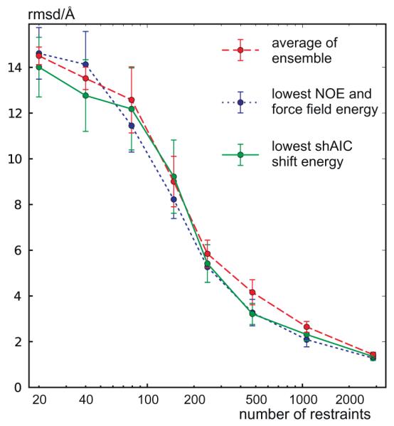
rmsd to reference structure as a function of the number of NOE restraints. An ensemble of structures was calculated for the protein with pdbID 1srr as described in Section 2.3.2 and the procedure was repeated to produce eight such ensembles each with eight structures, and again for all eight different groups using a different number of distance restraints. The rmsd to the reference structure is plotted for all eight members of the ensemble taking an average within the same ensemble (red curve), the member within each ensemble with lowest empirical target function combining NOE and force field energy (blue curve), and the member within each ensemble with lowest shAIC chemical shift pseudo energy (green curve). For each group with a different number of distance restraints, the standard deviation among the rmsds for the eight such best members (from the eight ensembles having the same number of distance restraints) are indicated by error bars. (For interpretation of the references to color in this figure legend, the reader is referred to the web version of this article.)
To quantify the relation between shift energy and structural quality further the full set of the structure decoys were combined comparing the shift energy with the reference rmsd. As shown in Fig. 17, there is a strong correlation between the shAIC energy (for a structure decoy) and the rmsd to the reference structure, with a squared Spearman’s rank correlation coefficient, R2 (Spearman), (a non-parametric measure of statistical dependence with a value of 1 indicating a perfect monotonically increasing relation) [79] of 0.952. Qualitatively, this strong correlation demonstrates the power to evaluate the correctness of protein structures by shAIC and suggests a possibility to conduct the reverse procedure of deriving the structure from the chemical shift. When using Sparta+ to calculate a similar energy a value of R2 (Spearman) = 0.936 is obtained indicating an almost similar relationship. However, it should be noted that, shAIC has a marginally better correlation between shift-energy and structure for structures far away from the real structure as compared to Sparta+. For example, for structures with rmsd > 6.0 Å, the R2 (Pearson) is 0.637 vs. 0.463 for shAIC vs. Sparta+. This implies that shAIC is more powerful at the start of the structure calculation, which is typically where chemical shift potentials are less sensitive.
Fig. 17.

The shAIC and Sparta+ normalized chemical shift energy score, Z, vs. rmsd deviation from the reference structure. In (a) each 2·256 points (blue and red dots for shAIC and Sparta+, respectively) represent a structure decoy calculated for one of the protein structures determined by X-ray from the ROSETTA test set, pdbID 1srr, (see Section 2.5). The chemical shift energy (Eq. (4)) was converted to a Z-score by subtracting the mean and dividing by the standard deviation shown on the y-axis. The secondary structure designation of each decoy was calculated using DSSP [51]. The rmsd deviation when overlayed with the reference X-ray structure is shown at the x-axis. In (b) the same relation is shown but with combining 16 consecutive structures with increasing rmsds to the reference structure and showing the mean rmsd and the mean score on the axes using the standard deviation within the 16 structures as error bars.
4.4.2. Smoothness and differentiability of the shAIC potential
shAIC uses analytical and differentiable potentials with continuous derivatives (such as a smooth spline model) as the basis for parameterization. As a result, shAIC potentials not only vary smoothly with internal parameters, but the differentials of the chemical shift energy can be computed in an explicit and examinable manner. The smoothness of the energy-surface makes it less likely for shAIC to get stuck in local minima when it is used as a proxy to explore energy landscapes. To illustrate this attractive feature, we evaluated the shAIC energy as a function of a systematic change in the backbone conformation corresponding to crank-shaft libration motion [80,81] to produce an energy profile (see Section 2) as shown in Fig. 18. An energy profile was calculated similarly for Sparta+ to compare with shAIC. It is observed that the shAIC energy profiles have a slightly sharper minimum and are also slightly smoother compared to the Sparta+ energy profiles. Furthermore, the minimum is closer to the observed backbone conformation. In addition to the advantage of offering a smoother energy landscape, shAIC offers a practical computational advantage. The smooth spline model allows for an explicit determination of differentials thereby reducing computational load and the potential for numerical instability in performing discrete differentiation.
Fig. 18.

(a) The shAIC and (b) Sparta+ chemical shift energy vs. the “crankshaft” deviation from the reference structure. shAIC (a) and Sparta+ (b) energy profiles. The energy calculated using Eq. (4) is shown as a function of the “crank-shaft” shift, θ, relative to the observed values in the structure (pdbid 1srr) for three consecutive residues 25–27 in a loop shown as blue, red and green curves, respectively. θ = 0 refers to the reference structure and θ = Δ to a modified structure with φ(i − 1) = φobs(i − 1) + Δ and ϕ(i)= ϕobs(i) − Δ (and all other angles unchanged). Such modified structures were produced in steps of 3°. Insert (b): the 40 different protein conformations used for calculating the profiles. The reference structure is shown in green and with a cartoon and with lines linking consecutive Cα atoms (Cα-trace) while the modified structures are shown in different colors with a Cα-trace only. The effect of a “crankshaft motion” is a local distortion near residue, i, along with a small translation of the half of the protein from residue, i. (For interpretation of the references to color in this figure legend, the reader is referred to the web version of this article.)
4.4.3. shAIC as a fast method
shAIC is currently implemented in python, which is an interpreted language, in order to afford increased flexibility for implementation of potential improvements. Nonetheless, shAIC’s calculation times are on par with Sparta. A quantitative comparison was made comparing the runtimes of Sparta, Sparta+, CamShift ShiftX and shAIC on a linux HP Intel Pentium 4 workstation equipped with two 3.0 GHz processors. The chemical shifts were predicted for 64 of the structures derived for the protein with pdbID 1SRR having 121 residues as described in Sections 2.5 and 4.4.4. The average of the runtime per structure for 64 structures was calculated. ShiftX is the fastest method with an average runtime of 0.7s per structure whereas Sparta is the slowest spending 20.0s on the prediction. ShAIC uses 13.7s while Sparta+ and CamShift are faster with 1.8s and 2.0s runtimes, respectively. More importantly, and for purposes of more interactive and online applications, shAIC calculations are sufficiently fast, thereby making the integration of shAIC with molecular dynamics calculations in the form of a “chemical shift potential” to aid in folding computationally practical. Should additional speed improvements become necessary, about an order of magnitude enhancements in speed may be achievable via a more standard machine-interpreted language, for example C or C++. Furthermore, shAIC, as opposed to other methods, uses primarily univariate potentials meaning that if shAIC would be implemented as part of an calculation engine that varies the torsion angles systematically, calculating the gradient in terms of varying a single dihedral angle would only require the re-evaluation of a subset of the potentials corresponding to the change of the dihedral angle in question and hence shAIC would be considerable fast compared to other methods.
4.4.4. shAIC as a method of choice for chemical shift aided structure calculation
Combining our findings for the performance of shAIC (high accuracy, precision, and the highest correlation between structural quality of NMR structures and chemical shift energy), shAIC’s smooth energy-surface (allowing for explicit calculation of derivatives), and reasonably fast computational speeds, we propose that shAIC should be the method of choice for chemical shift aided structure calculation. The higher sensitivity of shAIC for structures far away from the correct structure, leads us to expect that it could play an important tool for de novo structure calculation without the explicit use of fragments as templates. Moreover, with the extended span of geometric parameters offered by shAIC, we envisage that features such as long-range order can be determined by shAIC more effectively, which in turn could aid in the determination of more complex structures.
5. Conclusions
We have introduced a novel method for chemical shift prediction, shAIC, which extensively and judiciously incorporates local as well as long-range structure effects through appropriate definition of an optimal set of input geometric parameters. shAIC offers advances in improved accuracy, generalizability, transparency of interpretation, smooth representation, and parsimony when compared to existing methods. In specific instances, for example, the accuracy when predicting chemical shifts for X-ray structures, competitive tools, for example Sparta+, are available. However, when considering NMR structures, or structures only remotely related to the protein structures used for training the methods, shAIC performs better relative to Sparta+. The parsimonious selection criteria of shAIC parameters and the choice to include NMR models is likely to be a key factor in explaining the better performance of shAIC. This fact makes it likely that shAIC predictions would be more robust when applied to a larger class of protein structures – outside of the highly precise X-ray structures. On the methodological side, shAIC adopts a sum of contributions approach by including a large number of input parameters and then uses the Akaikes Information Criterion to weight and select the individual contributions for optimal results. This approach offers rigor for the judicious handling of statistical data. shAIC may be used directly for chemical shift predictions and through its differentiable potentials, it can be incorporated into conventional MD programs. We envisage that shAIC will find widespread applications for protein structure quality assessment and easier and more precise structure calculations, including cases for which traditional approaches may prove less than adequate.
Acknowledgements
We acknowledge support from the Danish National Research Foundation, the Lundbeck Foundation, Villum-Kann Rasmussen Fonden, and the Danish Center for Scientific Computing, and the FP7 BIONMR project.
Appendix A
A.1. Definition of all generalized angles
A set of different generalized angles θ1–θ34 are defined, which are the input parameters used in the torsion angle class. The two backbone torsion angles are set to: θ1 = ϕ(i) and θ2 = φ(i). θ3 is set to the dihedral angle through the four consecutive Cα carbons of residues i − 1, i, i + 1, and i + 2 (see Fig. 3). Virtual dihedral angles θ4–θ20 are defined in Table 2. Angles θ21–θ24 are bend angle defined through the three Cα carbons of residues i − j, i, i + j, for angles θ20+j for j = 1, 2, 3, 4.
Angles θ25–θ34 are defined only for helixes and β-sheets and are related to hydrogen bonding: θ25 and θ26 are virtual dihedral angles across hydrogen bonds defined by the four carbons: Cβ(i), Cα(i), Cα(k), Cβ(k), where the residue number, k, is the residue number of the hydrogen bonding partner as defined in the legend to Fig. 4, which depends on the secondary structure, s, and atom type (reference atom) n, and Hα3 is used in place of Cβ for Gly. For helixes the hydrogen bonding partner is the residue to which HN and O are hydrogen bonded, for θ25 and θ26, respectively, i.e. for example k = i − 4 and i + 4 for HN and C’, respectively. For sheets the definition differs for different atom types as defined in Fig. 4. For example, if n is HN or N the hydrogen bonding partner is the residue to which HN is hydrogen bonded. θ26 is the same angle as θ25 but using another residue in the opposite strand as the hydrogen bonding partner, e.g. if n is HN(i) or N(i) the other residue is the one to which the oxygen of C’(i − 1) is hydrogen bonded. Angles θ27, θ28 and θ29 are θNHO, θHOC and θDHOC of which the two former are defined in a legend to Tables 1 and 2 (using n as the reference atom). The dihedral angle, θNHOC is defined by the four atoms N(j), H(j), O(k), C’(k) using the same definition of the four atoms as for θNHO and θHOC, where k is the residue number of the hydrogen bonding partner, which is the same as the hydrogen bonding partner for θ25, D and H are N and HN except for n = Hα for which D = Cα and H = Hα are used. Angles θ30, θ31 and θ32 are the angles θNHO, θHOC and θDHOC using O(i − 1) as the reference atom (cf. Table 2) for n = HN or N and HN(i + 1) in the other cases. Finally, θ33 = ϕ(k) and θ34 = φ(k) where k, is the residue number of the hydrogen bonding partner as discussed above.
A.2. Tables of the pdb and bmr files
We provide here in Table A1 the IDs for pdb and bmr-files used for evaluating shAIC and other methods for predicting chemical shifts. The pdb and bmr-files used for training shAIC are given in Tables A2 and A3.
Table A1.
pdbID and bmrIDs and resolution (first three columns) for all members of the set of 38 chains used for evaluating shAIC (Section 2.5), the fifth character in the pdbID indicates the chain identifier with a “−” indicating a protein with only one single unique chain. In column 4 with the heading “NMR structure” the pdbID for the corresponding NMR structure used for the analysis in Fig. 7d is indicated. In column 5 with the heading “Sparta+ remote” a “+” indicates that this structure is one of the eight, used for the analysis in Fig. 7b, having less than 25% sequence identity with any chain in the set used for training Sparta+, whereas a “−” indicates that this structure was not used in this analysis.
| pdbID | bmrID | Resolution | NMR structure | Sparta+ remote |
|---|---|---|---|---|
| 1SUE_ | 15,248 | 1.8 | n.a. | − |
| 1QMYA | 15,278 | 1.9 | n.a. | − |
| 1TPH2 | 15,064 | 1.8 | n.a. | − |
| 1NQDA | 15,722 | 1.65 | n.a. | + |
| 2HZIB | 15,488 | 1.7 | n.a. | − |
| 2O0PA | 15,281 | 1.9 | 2JQN | − |
| 2DYIA | 10,138 | 2.0 | 2DOG | + |
| 1ZX8A | 16,007 | 1.9 | 2KA0 | − |
| 2PSTX | 7075 | 1.8 | 2GPF | − |
| 1QKRA | 15,653 | 1.8 | n.a. | − |
| 2OOAA | 15,111 | 1.56 | 2JNH | − |
| 2CA5B | 15,214 | 2.1 | n.a. | − |
| 2HDZA | 5392 | 2.0 | 1L8Y | − |
| 2GSVB | 15,350 | 1.9 | 2JS1 | + |
| 1Y9TA | 15,503 | 1.87 | n.a. | − |
| 1OMYA | 7330 | 2.0 | 2E0H | + |
| 1U06A | 7305 | 1.49 | 1AEY | − |
| 1KMVA | 7195 | 1.05 | 1YHO | − |
| 1IKOP | 7220 | 1.92 | 2I85 | − |
| 1FGZA | 15,669 | 2.05 | n.a. | − |
| 1IWMA | 10,096 | 1.9 | n.a. | − |
| 1ZYNA | 15,264 | 2.3 | n.a. | − |
| 1U4EA | 11,067 | 2.09 | n.a. | + |
| 2IONA | 6900 | 1.57 | 2HM8 | − |
| 2NNRA | 6876 | 1.7 | 2FO8 | − |
| 2CG6A | 15,756 | 1.55 | 2CKU | + |
| 2IN0A | 15,560 | 1.6 | n.a. | − |
| 1O5UA | 16,006 | 1.83 | 1LKN | − |
| 2A0NA | 15,741 | 1.64 | n.a. | − |
| 1EXP_ | 7264 | 1.8 | n.a. | − |
| 2ES9A | 15,089 | 2.0 | 2JN8 | + |
| 1YSBB | 6223 | 1.7 | n.a. | − |
| 2OYNA | 15,530 | 1.85 | 2P3 M | − |
| 1M8AB | 15,596 | 1.7 | 2JYO | − |
| 2UV0H | 6271 | 1.8 | n.a. | − |
| 1M1FA | 6925 | 1.4 | n.a. | − |
| 1BED_ | 7360 | 2.0 | n.a. | − |
| 1NAQC | 15,094 | 1.7 | n.a. | + |
Table A2.
pdbID and bmrIDs for all NMR structures from the shAIC training set of 681 protein chains. The table is folded providing pairs of corresponding bmr and pdb IDs in columns 1 + 2, 3 + 4, 5 + 6, 7 + 8 and 9 + 10.
| 1AAB_ | 4079 | 1H92A | 5223 | 1N9JA | 4827 | 1T0GA | 6138 | 1Z6HA | 6600 |
| 1ADNA | 6053 | 1HA8A | 4979 | 1NBLA | 5670 | 1T0YA | 6176 | 1Z7PA | 6410 |
| 1AOO_ | 4859 | 1HA9A | 5176 | 1NE3A | 5620 | 1T17A | 6120 | 1Z8RA | 6613 |
| 1APO_ | 1071 | 1HD6A | 4820 | 1NE5A | 5652 | 1T1HA | 6265 | 1ZDXA | 6779 |
| 1AQ5C | 4055 | 1HJ0A | 5257 | 1NER_ | 287 | 1T1TA | 6222 | 1ZK6A | 6601 |
| 1AUUB | 4095 | 1HLLA | 5143 | 1NG7A | 5753 | 1T2YA | 6290 | 1ZR7A | 6721 |
| 1AXH_ | 5702 | 1HQBA | 4603 | 1NI7A | 5630 | 1T4ZA | 5141 | 1ZU2A | 6626 |
| 1AZ6_ | 4057 | 1HS5B | 4934 | 1NNVA | 5779 | 1TBAA | 4223 | 1ZW8A | 6648 |
| 1B1VA | 4292 | 1HVWA | 4937 | 1NO8A | 5764 | 1TH5A | 6247 | 1ZXAB | 1757 |
| 1B2TA | 4397 | 1HY8A | 4989 | 1NQ4A | 5664 | 1TI5A | 6525 | 1ZZPA | 6570 |
| 1B64_ | 4117 | 1I11A | 5036 | 1NTCB | 4348 | 1TIZA | 6209 | 2A00A | 6029 |
| 1BA5A | 4210 | 1I25A | 4988 | 1NXIA | 5589 | 1TKVA | 4040 | 2A3JA | 6493 |
| 1BBL_ | 2546 | 1I26A | 5039 | 1NY8A | 5798 | 1TL4A | 6266 | 2A4HA | 6738 |
| 1BCI_ | 4188 | 1I2VA | 4976 | 1NY9A | 5706 | 1TOTA | 6238 | 2A55A | 6712 |
| 1BF8A | 4070 | 1I8HB | 4882 | 1NYPA | 5692 | 1TQZA | 6354 | 2A7YA | 7000 |
| 1BHA_ | 2580 | 1I8XA | 4351 | 1NZPA | 5766 | 1TTVA | 6248 | 2AFEA | 6751 |
| 1BHU_ | 4217 | 1ICA_ | 1209 | 1O6XA | 5561 | 1TUJA | 5030 | 2AFPA | 4452 |
| 1BK8_ | 4163 | 1ICHA | 5018 | 1O8RA | 5603 | 1TUZA | 6208 | 2AGMA | 6390 |
| 1BPV_ | 4295 | 1IE5A | 5044 | 1OH1A | 5810 | 1TVJA | 5177 | 2AHQA | 6816 |
| 1BQZ_ | 4227 | 1IEHA | 4969 | 1OM2A | 4496 | 1U5MA | 6299 | 2AIZP | 6465 |
| 1BV8A | 4168 | 1IFWA | 5053 | 1OMUA | 5473 | 1UC6A | 5126 | 2AKKA | 6746 |
| 1BW5_ | 4121 | 1IJZA | 5004 | 1OP4A | 5786 | 1UEOA | 5806 | 2AL3A | 6761 |
| 1BXLA | 6578 | 1IRZA | 5174 | 1OQAA | 6114 | 1UFMA | 5849 | 2AMNA | 6835 |
| 1BZBA | 4219 | 1ITFA | 4081 | 1OQKA | 5710 | 1UGLA | 5848 | 2AMWA | 6769 |
| 1C06A | 4577 | 1IW4A | 5348 | 1OV2A | 5598 | 1UHUA | 5880 | 2APNA | 5963 |
| 1C20A | 4334 | 1IX5A | 4668 | 1OVXA | 5665 | 1UKXA | 6297 | 2ARFA | 6914 |
| 1C6WA | 4696 | 1IYCA | 5491 | 1OWXA | 5235 | 1UUCA | 6110 | 2ASWA | 6822 |
| 1C8AA | 4449 | 1IYMA | 5459 | 1P68A | 5687 | 1UW0A | 6035 | 2ASYB | 6868 |
| 1CCVA | 4422 | 1IYTA | 6554 | 1P6SA | 5778 | 1UW2A | 6097 | 2AVGA | 6015 |
| 1CE3A | 4487 | 1J0TA | 5653 | 1P6TA | 5813 | 1UZCA | 5537 | 2AVXA | 6454 |
| 1CFE_ | 4301 | 1J2NA | 5662 | 1P7AA | 5851 | 1V06A | 5884 | 2AXLA | 6540 |
| 1CIXA | 5268 | 1J7HC | 5606 | 1P7MA | 5668 | 1V66A | 6072 | 2AYJA | 6747 |
| 1CKXA | 4596 | 1J7MA | 5012 | 1P8AA | 5850 | 1VD0A | 5807 | 2AZHA | 6362 |
| 1CLHA | 4037 | 1J8KA | 5027 | 1PA4A | 5796 | 1VD8A | 6157 | 2B38A | 6872 |
| 1CMZA | 4407 | 1J9IA | 4752 | 1PB5A | 5817 | 1VDYA | 5928 | 2B5XA | 6847 |
| 1CPZA | 4344 | 1JAJA | 5010 | 1PBA_ | 979 | 1VEEA | 5929 | 2B68A | 6849 |
| 1CW6A | 4507 | 1JBIA | 5047 | 1PD7B | 5457 | 1VKRA | 6267 | 2B7EA | 6850 |
| 1CX1A | 4706 | 1JH3A | 5070 | 1PJZA | 5820 | 1VMPA | 4852 | 2B86A | 6854 |
| 1CZ5A | 4376 | 1JJDA | 5147 | 1PU1A | 5704 | 1VPC_ | 4257 | 2B95B | 6527 |
| 1D8KA | 4721 | 1JJGA | 5077 | 1PUZA | 5846 | 1VYNA | 5999 | 2BBG_ | 4211 |
| 1DAVA | 4524 | 1JKNA | 4448 | 1PV0A | 5847 | 1W1NA | 6228 | 2BBUA | 6580 |
| 1DBDB | 4087 | 1JLZA | 5082 | 1PV3A | 5677 | 1W7EA | 6312 | 2BBXA | 6865 |
| 1DCJA | 4819 | 1JO6A | 5092 | 1Q56A | 4978 | 1WCJA | 5976 | 2BGOA | 6475 |
| 1DE3A | 4158 | 1JR6A | 4791 | 1Q5FA | 5879 | 1WGKA | 6337 | 2BO5A | 6564 |
| 1DF6A | 4461 | 1JRMA | 5104 | 1Q71A | 5859 | 1WJDB | 10,015 | 2BRZ_ | 5723 |
| 1DKCA | 4615 | 1JRUA | 5155 | 1QK7A | 4410 | 1WKT_ | 5255 | 2BVBA | 6376 |
| 1DL0A | 4685 | 1JU8A | 5098 | 1QK9A | 4280 | 1WLXA | 6013 | 2CUJA | 6781 |
| 1DP3A | 4584 | 1JW2A | 5166 | 1QKYA | 4427 | 1WO3A | 6329 | 2D3JA | 6840 |
| 1DPUA | 4460 | 1JW3A | 5165 | 1QLZA | 4641 | 1WPIA | 6345 | 2D82A | 6960 |
| 1DQCA | 4290 | 1JXCA | 5056 | 1QUWA | 5241 | 1WQKA | 6370 | 2DEZA | 7006 |
| 1DU9A | 4585 | 1K42A | 5181 | 1QXFA | 5682 | 1WQUA | 6331 | 2DK9A | 7058 |
| 1DUJA | 4775 | 1K7BA | 5210 | 1QXNB | 4776 | 1WU0A | 6489 | 2DMMA | 4908 |
| 1DV0A | 4757 | 1KA5A | 2030 | 1R21A | 5959 | 1X32A | 6589 | 2EXNA | 6693 |
| 1E3YA | 4333 | 1KG1A | 5199 | 1R2AB | 4473 | 1X9BA | 6291 | 2EZH_ | 4090 |
| 1EGXA | 5754 | 1KJ0A | 5274 | 1R57A | 5845 | 1XAXA | 5942 | 2F05A | 6899 |
| 1EHXA | 4589 | 1KJS_ | 2506 | 1R6RB | 5973 | 1XDXB | 4929 | 2F1EA | 5998 |
| 1EIJA | 4674 | 1KKGA | 5093 | 1R73A | 5977 | 1XHJA | 6355 | 2F8BA | 6916 |
| 1EIKA | 4678 | 1KLRA | 1500 | 1RGWA | 5696 | 1XHSA | 6448 | 2FB7A | 7084 |
| 1EIOA | 4673 | 1KMXA | 5238 | 1RHWA | 6096 | 1XKEA | 5159 | 2FFKA | 6809 |
| 1EL0A | 4686 | 1KN6A | 5242 | 1RI0A | 5902 | 1XN5A | 6369 | 2FFTA | 6926 |
| 1EMXA | 4755 | 1KRIA | 5275 | 1RJIA | 6037 | 1XN7A | 6367 | 2FFWA | 6920 |
| 1EMZA | 4699 | 1KV4A | 5265 | 1RJVA | 6049 | 1XN9A | 6368 | 2FI2A | 6957 |
| 1EOQA | 4593 | 1KVZA | 4893 | 1RKLA | 6056 | 1XNAA | 4282 | 2FK4A | 6407 |
| 1ERQA | 6357 | 1L1IA | 5323 | 1RL1A | 6012 | 1XNEA | 6364 | 2FNFX | 6059 |
| 1EV0B | 4237 | 1L1PA | 5298 | 1RMKA | 6135 | 1XOYA | 6341 | 2FQCA | 6951 |
| 1F2HA | 4636 | 1L2MA | 5297 | 1RQ6A | 6028 | 1XPA_ | 4249 | 2FXPC | 6969 |
| 1F2RC | 4451 | 1L3GA | 4254 | 1RQ8A | 5763 | 1XS3A | 6358 | 2FY9B | 6826 |
| 1F53A | 4758 | 1L3HA | 5583 | 1RRZA | 6108 | 1XSCA | 6336 | 2GGRA | 7129 |
| 1F81A | 4789 | 1L3YA | 5338 | 1RW2A | 5907 | 1XU6A | 6419 | 2GJIA | 7099 |
| 1FEXA | 4639 | 1L7YA | 5329 | 1RW5A | 6643 | 1XWEA | 6001 | 2GLOA | 7134 |
| 1FJ7A | 4858 | 1LBJA | 754 | 1RY4A | 6126 | 1XX3A | 6375 | 2GM2A | 7054 |
| 1FJCA | 4863 | 1LFC_ | 4157 | 1RZSA | 6185 | 1Y6UA | 6479 | 2GOVA | 6620 |
| 1FQQA | 4642 | 1LL8A | 5354 | 1S6DA | 6082 | 1Y7NA | 6113 | 2GS0A | 6225 |
| 1FU9A | 4939 | 1LMMA | 5495 | 1S6LA | 6047 | 1Y7XA | 6447 | 2GUTA | 7185 |
| 1FV5A | 4644 | 1LO1A | 4034 | 1S6UA | 6130 | 1YELA | 6464 | 2GWPA | 6264 |
| 1FWOA | 4645 | 1LQC_ | 2956 | 1S8KA | 6109 | 1YEZA | 6505 | 2H3KA | 6759 |
| 1FZTA | 4648 | 1M2FA | 5031 | 1SA8A | 6134 | 1YHDA | 6453 | 2HDLA | 7229 |
| 1G03A | 4649 | 1M36A | 5464 | 1SB6A | 6172 | 1YKGA | 4985 | 2HPUA | 5595 |
| 1G2HA | 4784 | 1M4FA | 5501 | 1SE9A | 6128 | 1YQAA | 6476 | 2HYMA | 5049 |
| 1G4FA | 4981 | 1MB6A | 5527 | 1SG7A | 6117 | 1YTRA | 6561 | 2IDAA | 7297 |
| 1G5VA | 4899 | 1MG8A | 5496 | 1SH1_ | 275 | 1YUA_ | 4045 | 2IN2A | 5659 |
| 1G7OA | 4318 | 1MHU_ | 4684 | 1SJ6A | 6152 | 1YUTA | 6531 | 2IZ4A | 5565 |
| 1G9PA | 4923 | 1MSZA | 5535 | 1SJQA | 6178 | 1YWSA | 6555 | 2KTX_ | 6351 |
| 1GHTA | 4269 | 1MV4B | 5610 | 1SJRA | 6177 | 1YWWA | 6517 | 2MFN_ | 4206 |
| 1GNFA | 4423 | 1MVZA | 5617 | 1SNLA | 6167 | 1YX3A | 6518 | 2MOBA | 4486 |
| 1GO5A | 5364 | 1N0ZA | 5667 | 1SR2A | 6133 | 1YYBA | 6556 | 2XBD_ | 4241 |
| 1GXEA | 5014 | 1N4YA | 5949 | 1SRKA | 6216 | 1YZBA | 6241 | 3NCMA | 4143 |
| 1H20A | 1918 | 1N6ZA | 5568 | 1SSLA | 6165 | 1Z2KA | 6538 | 8TFVA | 4387 |
| 1H3ZA | 5538 | 1N87A | 5594 | 1SXDA | 6287 | 1Z3RA | 6309 | ||
| 1H67A | 4880 | 1N88A | 5650 | 1SXL_ | 4085 | 1Z65A | 6598 |
Table A3.
pdbID and bmrIDs and resolution for all structures determined by X-ray from the shAIC training set of 681 protein chains. The table is folded proving triplets of corresponding bmr and pdb IDs and resolution in columns 1 + 2 + 3, 4 + 5 + 6, 7 + 8 + 9.
| 1A2PA | 4964 | 1.50 | 1I5ZA | 4388 | 2.10 | 1TP9A | 6132 | 1.62 |
| 1ABA_ | 4459 | 1.45 | 1IAZA | 4797 | 1.90 | 1TTZA | 6363 | 2.11 |
| 1AE3A | 2039 | 2.00 | 1IPCA | 7115 | 2.00 | 1TUKA | 4977 | 1.12 |
| 1AG6_ | 79 | 1.60 | 1IRFA | 4161 | 2.20 | 1TVGA | 6344 | 1.60 |
| 1AILA | 4317 | 1.90 | 1IU1A | 5761 | 1.80 | 1UB4B | 6828 | 1.70 |
| 1AJ6_ | 5218 | 2.30 | 1IV7A | 4638 | 1.82 | 1UDRD | 4083 | 1.90 |
| 1AR0A | 5888 | 2.30 | 1IWTA | 5142 | 1.40 | 1UHIB | 6418 | 1.80 |
| 1ARRA | 395 | 1.90 | 1J1VA | 5200 | 2.10 | 1UJ8A | 6776 | 1.75 |
| 1ASS_ | 5930 | 2.30 | 1J3FA | 4568 | 1.45 | 1UOHA | 5898 | 2.00 |
| 1B2VA | 5081 | 1.90 | 1J54A | 6184 | 1.70 | 1UP1_ | 4084 | 1.90 |
| 1B40A | 5909 | 2.2 | 1J8RA | 4897 | 1.80 | 1UTXB | 6317 | 1.90 |
| 1B68A | 6524 | 2.00 | 1JF8A | 4944 | 1.12 | 1UUGB | 4044 | 2.40 |
| 1B9KA | 6034 | 1.9 | 1JHFA | 6373 | 1.80 | 1UUHA | 6093 | 2.20 |
| 1BDO_ | 4426 | 1.80 | 1JIWI | 6292 | 1.74 | 1UV0A | 6231 | 1.78 |
| 1BFC_ | 4091 | 2.20 | 1JNJA | 5783 | 2.50 | 1V2ZA | 5824 | 1.80 |
| 1BGQ_ | 5355 | 2.50 | 1JOCA | 4579 | 2.20 | 1VAPB | 4078 | 1.60 |
| 1BJAB | 4957 | 2.19 | 1JRLA | 4060 | 1.95 | 1VC1A | 5921 | 2.00 |
| 1BQ8A | 1991 | 1.10 | 1K82A | 5219 | 2.10 | 1VJHB | 6585 | 2.10 |
| 1BWOB | 4383 | 2.10 | 1KATV | 5185 | 1.93 | 1VYFA | 6150 | 1.85 |
| 1BY9A | 5952 | 2.20 | 1KJLA | 4909 | 1.40 | 1W41A | 5485 | 1.70 |
| 1BYFA | 4782 | 2.00 | 1KTZA | 4411 | 2.15 | 1WKXA | 6123 | 1.70 |
| 1BYLA | 4786 | 2.30 | 1KTZB | 4779 | 2.15 | 1WYWB | 6304 | 2.10 |
| 1C44A | 4438 | 1.80 | 1KX9B | 5094 | 1.65 | 1X8RA | 4848 | 1.50 |
| 1C76A | 4215 | 2.25 | 1L0SB | 5573 | 2.30 | 1X8UC | 4267 | 2.20 |
| 1CEX_ | 4101 | 1.00 | 1L1DB | 6051 | 1.85 | 1XDGA | 4553 | 2.10 |
| 1CKUB | 2999 | 1.20 | 1LBDA | 6429 | 1.90 | 1XEOA | 5404 | 1.30 |
| 1CLVI | 4404 | 2.00 | 1LP1B | 4324 | 2.30 | 1XMTA | 6338 | 1.15 |
| 1CM2A | 2371 | 1.80 | 1M15A | 6542 | 1.20 | 1XZOA | 5742 | 1.70 |
| 1CNR_ | 6504 | 1.05 | 1M5AB | 1444 | 1.20 | 1Y62C | 6506 | 2.45 |
| 1COMA | 6494 | 2.20 | 1MFTA | 6302 | 2.50 | 1Y93A | 6391 | 1.03 |
| 1CRB_ | 5579 | 2.10 | 1MHOA | 5206 | 2.00 | 1YCEA | 4316 | 2.40 |
| 1CY5A | 4661 | 1.30 | 1MJC_ | 4296 | 2.00 | 1YJ7A | 6252 | 1.80 |
| 1D8CA | 5471 | 2.0 | 1MSPA | 4242 | 2.50 | 1YP7A | 4340 | 2.00 |
| 1DCDB | 5249 | 2.00 | 1MVKD | 5654 | 2.50 | 1YU7X | 4428 | 1.50 |
| 1DFUP | 4395 | 1.80 | 1N0SA | 5756 | 2.00 | 1YY6A | 6939 | 1.70 |
| 1DHNA | 4573 | 1.65 | 1NBPA | 6621 | 2.20 | 1ZLQB | 6416 | 1.80 |
| 1DXWA | 4617 | 2.40 | 1ND4A | 5721 | 2.10 | 1ZQW_ | 5208 | 2.30 |
| 1E0CA | 7130 | 1.80 | 1NG2A | 6057 | 1.70 | 1ZYJA | 6468 | 2.00 |
| 1E4VA | 4193 | 1.85 | 1NGA_ | 6628 | 1.30 | 2A0B_ | 4857 | 1.57 |
| 1EB0A | 5484 | 1.85 | 1NOA_ | 1766 | 1.50 | 2A38C | 5760 | 2.00 |
| 1EDHB | 4380 | 2.00 | 1O13A | 6198 | 1.83 | 2A3GA | 1442 | 2.25 |
| 1EDNA | 194 | 2.18 | 1O82D | 4112 | 1.46 | 2ADFA | 5456 | 1.90 |
| 1EHBA | 294 | 1.90 | 1OBOA | 5011 | 1.20 | 2AHPB | 371 | 2.00 |
| 1EJFB | 6973 | 2.49 | 1OC0B | 6160 | 2.28 | 2B02A | 6597 | 1.50 |
| 1EK8A | 5190 | 2.30 | 1ODVA | 6321 | 1.14 | 2B59A | 5267 | 2.11 |
| 1EKGA | 4342 | 1.80 | 1ONJA | 5690 | 1.55 | 2B8XA | 4094 | 1.70 |
| 1EMVA | 4115 | 1.70 | 1OQRC | 4149 | 1.65 | 2B9AA | 5507 | 1.54 |
| 1EPFC | 4162 | 1.85 | 1OSPO | 4076 | 1.95 | 2BF5B | 4560 | 1.71 |
| 1ET1A | 1666 | 0.90 | 1OVHA | 915 | 1.95 | 2BJDA | 6398 | 1.27 |
| 1EW4A | 5792 | 1.40 | 1P6ZN | 916 | 1.67 | 2BYFA | 6635 | 1.90 |
| 1EZ9A | 6807 | 1.90 | 1Q4RA | 5843 | 1.90 | 2C2HA | 6970 | 1.85 |
| 1F35A | 4735 | 2.30 | 1QE6A | 280 | 2.35 | 2C6YA | 4829 | 2.40 |
| 1F46A | 4717 | 1.50 | 1QFJC | 7138 | 2.20 | 2CI2I | 4974 | 2.00 |
| 1F5WA | 5516 | 1.7 | 1QJ8A | 4936 | 1.90 | 2CIAA | 6575 | 1.45 |
| 1F94A | 5097 | 0.97 | 1QMRA | 4417 | 2.15 | 2D3DA | 6922 | 1.60 |
| 1FF3C | 6090 | 1.90 | 1QOGA | 447 | 1.80 | 2END_ | 5244 | 1.45 |
| 1FIL_ | 4082 | 2.00 | 1QSTA | 4321 | 1.70 | 2ESPA | 6277 | 1.52 |
| 1G4CB | 4299 | 1.65 | 1QVEA | 4918 | 1.54 | 2EWRA | 7086 | 1.60 |
| 1G6HA | 5462 | 1.60 | 1R5RA | 4940 | 1.60 | 2F1NA | 6758 | 1.73 |
| 1G7FA | 5474 | 1.80 | 1R69_ | 2539 | 2.00 | 2FJYA | 4849 | 2.30 |
| 1G8IB | 4378 | 1.90 | 1R7JA | 5891 | 1.47 | 2FKE_ | 4077 | 1.72 |
| 1GAWA | 6695 | 2.20 | 1RGHB | 5492 | 1.20 | 2FUFA | 4127 | 1.45 |
| 1GNUA | 5058 | 1.75 | 1RN1B | 1658 | 1.84 | 2FX5A | 6832 | 1.80 |
| 1GXQA | 4421 | 2.00 | 1RUWA | 6197 | 1.80 | 2GFEA | 5182 | 1.54 |
| 1H0AA | 4959 | 1.70 | 1RX4_ | 5741 | 2.20 | 2GHYA | 4072 | 2.50 |
| 1H0XA | 5226 | 1.70 | 1S0PA | 5393 | 1.40 | 2GOLD | 5258 | 2.20 |
| 1H4GA | 5352 | 1.10 | 1S7AA | 6044 | 1.85 | 2GTGA | 5465 | 2.40 |
| 1H70A | 6074 | 1.80 | 1SGZA | 6016 | 2.00 | 2H30A | 6709 | 1.60 |
| 1HB8B | 2049 | 2.00 | 1SKOB | 6181 | 2.00 | 2H9HA | 4836 | 1.39 |
| 1HCB_ | 4022 | 1.60 | 1SMXB | 6122 | 1.80 | 2PSPB | 2384 | 1.90 |
| 1HH8A | 6399 | 1.80 | 1SNM_ | 4053 | 1.74 | 3RN3_ | 4031 | 1.45 |
| 1HL5J | 6821 | 1.80 | 1SZ9A | 6404 | 2.10 | 3SSIA | 4331 | 2.30 |
| 1HOE_ | 60 | 2.00 | 1T2WB | 4879 | 1.80 | 451C_ | 1333 | 1.60 |
| 1HPCB | 4336 | 2.00 | 1T3YA | 6032 | 1.15 | 4TGF_ | 246 | 2.50 |
| 1HRHB | 5931 | 2.40 | 1THQA | 6234 | 1.90 | 5CROB | 1743 | 2.30 |
| 1HURA | 5368 | 2.00 | 1TJMA | 5194 | 1.18 | 5PTIA | 5359 | 1.0 |
| 1HUUB | 4047 | 2.00 | 1TOOA | 434 | 2.10 | 8ABP_ | 6136 | 1.49 |
| 1I1JB | 4731 | 1.39 | 1TP5A | 6193 | 1.54 |
References
- [1].Spera S, Bax A. J. Am. Chem. Soc. 1991;113:5490–5492. [Google Scholar]
- [2].Wishart DS, Sykes BD, Richards FM. J. Mol. Biol. 1991;222:311–333. doi: 10.1016/0022-2836(91)90214-q. [DOI] [PubMed] [Google Scholar]
- [3].Wishart DS, Bigam CG, Holm A, Hodges RS, Sykes BD. J. Biomol. NMR. 1995;5:67–81. doi: 10.1007/BF00227471. [DOI] [PubMed] [Google Scholar]
- [4].Osapay K, Case DA. J. Am. Chem. Soc. 1991;113:9436–9444. [Google Scholar]
- [5].Cavalli A, Salvatella X, Dobson CM, Vendruscolo M. Proc. Natl. Acad. Sci. USA. 2007;104:9615–9620. doi: 10.1073/pnas.0610313104. [DOI] [PMC free article] [PubMed] [Google Scholar]
- [6].Shen Y, Lange O, Delaglio F, Rossi P, Aramini JM, Liu GH, Eletsky A, Wu YB, Singarapu KK, Lemak A, Ignatchenko A, Arrowsmith CH, Szyperski T, Montelione GT, Baker D, Bax A. Proc. Natl. Acad. Sci. USA. 2008;105:4685–4690. doi: 10.1073/pnas.0800256105. [DOI] [PMC free article] [PubMed] [Google Scholar]
- [7].Wishart DS, Arndt D, Berjanskii M, Tang P, Zhou J, Lin G. Nucl. Acids Res. 2008;36:W496–W502. doi: 10.1093/nar/gkn305. [DOI] [PMC free article] [PubMed] [Google Scholar]
- [8].Reid LS, Thornton JM. Proteins. 1989;5:170–182. doi: 10.1002/prot.340050212. [DOI] [PubMed] [Google Scholar]
- [9].Summers NL, Karplus M. J. Mol. Biol. 1990;216:991–1016. doi: 10.1016/S0022-2836(99)80016-3. [DOI] [PubMed] [Google Scholar]
- [10].Bernstein FC, Koetzle TF, Williams GJB, Meyer EF, Brice MD, Rodgers JR, Kennard O, Shimanouchi T, Tasumi M. J. Mol. Biol. 1977;112:535–542. doi: 10.1016/s0022-2836(77)80200-3. [DOI] [PubMed] [Google Scholar]
- [11].Faraggi E, Yang YD, Zhang SS, Zhou YQ. Structure. 2009;17:1515–1527. doi: 10.1016/j.str.2009.09.006. [DOI] [PMC free article] [PubMed] [Google Scholar]
- [12].Robustelli P, Cavalli A, Dobson CM, Vendruscolo M, Salvatella X. J. Phys. Chem. B. 2009;113:7890–7896. doi: 10.1021/jp900780b. [DOI] [PubMed] [Google Scholar]
- [13].de Dios AC, Pearson JG, Pearson E, Oldfield Science. 1993;260:1491–1496. doi: 10.1126/science.8502992. [DOI] [PubMed] [Google Scholar]
- [14].Le HB, Pearson JG, de Dios AC, Oldfield E. J. Am. Chem. Soc. 1995;117:3800–3807. [Google Scholar]
- [15].de Dios AC. Prog. Nucl. Magn. Reson. Spectrosc. 1996;29:229–278. [Google Scholar]
- [16].Oldfield E. J. Biol. NMR. 1995;5:217–225. doi: 10.1007/BF00211749. [DOI] [PubMed] [Google Scholar]
- [17].Lazzeretti P. Ring currents. Prog. Nucl. Magn. Reson. Spectrosc. 2000;36:1–88. [Google Scholar]
- [18].Case DA. Curr. Opin. Struct. Biol. 1998;8:624–630. doi: 10.1016/s0959-440x(98)80155-3. [DOI] [PubMed] [Google Scholar]
- [19].Sternberg U, Witter R, Ulrich AS. Advances in Solid State NMR Studies of Materials, Polymers: A Special Volume Dedicated to Isao Ando. Academic Press Ltd.; London: 2004. 3D structure elucidation using NMR chemical shifts; pp. 53–104. [Google Scholar]
- [20].Xu XP, Case DA. J. Biomol. NMR. 2001;21:321–333. doi: 10.1023/a:1013324104681. [DOI] [PubMed] [Google Scholar]
- [21].Vila JA, Arnautova YA, Martin OA, Scheraga HA. Proc. Natl. Acad. Sci. USA. 2009;106:16972–16977. doi: 10.1073/pnas.0908833106. [DOI] [PMC free article] [PubMed] [Google Scholar]
- [22].Meiler J. J. Biomol. NMR. 2003;26:25–37. doi: 10.1023/a:1023060720156. [DOI] [PubMed] [Google Scholar]
- [23].Shen Y, Bax A. J. Biomol. NMR. 2010;48:13–22. doi: 10.1007/s10858-010-9433-9. [DOI] [PMC free article] [PubMed] [Google Scholar]
- [24].Moody JE. The effective number of parameters – an analysis of generalization and regularization in nonlinear learning-systems. In: Moody JE, Hanson SJ, Lippmann RP, editors. Advances in Neural Information Processing Systems. Vol. 4. Morgan Kaufmann Pub Inc.; San Mateo: 1992. pp. 847–854. [Google Scholar]
- [25].Weigend AS. Proceedings of the 1993 Connectionist Models Summer School.1994. pp. 335–342. [Google Scholar]
- [26].Shen Y, Delaglio F, Cornilescu G, Bax A. J. Biomol. NMR. 2009;44:213–223. doi: 10.1007/s10858-009-9333-z. [DOI] [PMC free article] [PubMed] [Google Scholar]
- [27].Lejewski C, Goodman N. J. Philos. Sci. 1959;9:331–333. [Google Scholar]
- [28].Wolpert DH. Math. General. 1995;20:117–214. [Google Scholar]
- [29].Wolpert DH. Neural Comput. 1996;8:1341–1390. [Google Scholar]
- [30].Hume D. In: A Treatise of Human Nature. Selby-Bigge LAN, Nidditch PH, editors. Oxford University Press; Oxford: 1978. [Google Scholar]
- [31].Kohlhoff KJ, Robustelli P, Cavalli A, Salvatella X, Vendruscolo M. J. Am. Chem. Soc. 2009;131:13894–13895. doi: 10.1021/ja903772t. [DOI] [PubMed] [Google Scholar]
- [32].Neal S, Nip AM, Zhang HY, Wishart DS. J. Biomol. NMR. 2003;26:215–240. doi: 10.1023/a:1023812930288. [DOI] [PubMed] [Google Scholar]
- [33].Shen Y, Bax A. J. Biomol. NMR. 2007;38:289–302. doi: 10.1007/s10858-007-9166-6. [DOI] [PubMed] [Google Scholar]
- [34].Akaike H. New look at statistical-model identification. IEEE Trans. Autom. Control. 1974;AC19:716–723. [Google Scholar]
- [35].Akaike H. Prediction and entropy. In: Atkinson ACF, Fienberg SE, editors. A Celebration of Statistics. Springer; New York: 1985. pp. 1–24. [Google Scholar]
- [36].Wishart DS. Prog. Nucl. Magn. Reson. Spectrosc. 2011;58:62–87. doi: 10.1016/j.pnmrs.2010.07.004. [DOI] [PubMed] [Google Scholar]
- [37].Robustelli P, Cavalli A, Vendruscolo M. Structure. 2008;16:1764–1769. doi: 10.1016/j.str.2008.10.016. [DOI] [PubMed] [Google Scholar]
- [38].Seidel K, Etzkorn M, Schneider R, Ader C, Baldus M. Solid State NMR. 2009;35:235–242. doi: 10.1016/j.ssnmr.2008.12.008. [DOI] [PubMed] [Google Scholar]
- [39].Wishart DS, Case DA. Methods in Enzymology. Academic Press; 2002. pp. 3–34. [DOI] [PubMed] [Google Scholar]
- [40].Christensen O. An Introduction to Frames and Riesz Bases. Birkhäuser; 2003. [Google Scholar]
- [41].Zhang HY, Neal S, Wishart DS. J. Biomol. NMR. 2003;25:173–195. doi: 10.1023/a:1022836027055. [DOI] [PubMed] [Google Scholar]
- [42].Carstens BC, Stoute HN, Reid N. Mol. Ecol. 2009;18:4270–4282. doi: 10.1111/j.1365-294X.2009.04327.x. [DOI] [PubMed] [Google Scholar]
- [43].Schwarz G. Ann. Statist. 1978;6:461–464. [Google Scholar]
- [44].Shao J. J. Am. Statist. Asso. 1993;88:486–494. [Google Scholar]
- [45].Shao J. Statist. Sinica. 1997;7:221–242. [Google Scholar]
- [46].Stone M. Biometrika. 1977;64:29–35. [Google Scholar]
- [47].Stone M. J. R. Statist. Soc. B. 1977;39:44–47. [Google Scholar]
- [48].Shao JT, Tu D. The Jackknife and Bootstrap. Springer-Verlag; New York: 1995. [Google Scholar]
- [49].Snijders TAB. On cross-validation for predictor evaluation in time series. In: Dijkstra Theo K., editor. On Model Uncertainty and its Statistical Implications. Vol. 307. Springer; Berlin: 1988. pp. 56–69. (Lecture Notes in Economics and Mathematical Systems). [Google Scholar]
- [50].Stone M. J. R. Statist. Soc. B. 1979;41:276–278. [Google Scholar]
- [51].Kabsch W, Sander C. Biopolymers. 1983;22:2577–2637. doi: 10.1002/bip.360221211. [DOI] [PubMed] [Google Scholar]
- [52].Schwieters CD, Kuszewski JJ, Tjandra N, Clore GM. J. Magn. Reson. 2003;160:65–73. doi: 10.1016/s1090-7807(02)00014-9. [DOI] [PubMed] [Google Scholar]
- [53].Kuszewski J, Clore GM. J. Magn. Reson. 2000;146:249–254. doi: 10.1006/jmre.2000.2142. [DOI] [PubMed] [Google Scholar]
- [54].Kuszewski J, Gronenborn AM, Clore GM. J. Am. Chem. Soc. 1999;121:2337–2338. [Google Scholar]
- [55].Schoenberg IJ. Q. Appl. Math. 1946;4:45–99. [Google Scholar]
- [56].Pople JA. J. Chem. Phys. 1956;24:1111. [Google Scholar]
- [57].Moyna G, Zauhar RJ, Williams HJ, Nachman RJ, Scott AI. J. Chem. Inf. Comput. Sci. 1998;38:702–709. doi: 10.1021/ci980402e. [DOI] [PubMed] [Google Scholar]
- [58].Hobohm U, Scharf M, Schneider R, Sander C. Protein Sci. 1992;1:409–417. doi: 10.1002/pro.5560010313. [DOI] [PMC free article] [PubMed] [Google Scholar]
- [59].Word JM, Lovell SC, Richardson JS, Richardson DC. J. Mol. Biol. 1999;285:1735–1747. doi: 10.1006/jmbi.1998.2401. [DOI] [PubMed] [Google Scholar]
- [60].Painter J, Merritt EA. J. Appl. Crystallogr. 2004;37:174–178. [Google Scholar]
- [61].Cock PJA, Antao T, Chang JT, Chapman BA, Cox CJ, Dalke A, Friedberg I, Hamelryck T, Kauff F, Wilczynski B, de Hoon MJL. Bioinformatics. 2009;25:1422–1423. doi: 10.1093/bioinformatics/btp163. [DOI] [PMC free article] [PubMed] [Google Scholar]
- [62].Krissinel E, Henrick K. J. Mol. Biol. 2007;372:774–797. doi: 10.1016/j.jmb.2007.05.022. [DOI] [PubMed] [Google Scholar]
- [63].Canal L. Comput. Statist. Data Anal. 2005;48:803–808. [Google Scholar]
- [64].Levenberg K. Q. Appl. Math. 1944;2:164–168. [Google Scholar]
- [65].Marquardt DW. J. Soc. Ind. Appl. Math. 1963;11:431–441. [Google Scholar]
- [66].Nelder JA, Mead R. Comput. J. 1965;7:308–313. [Google Scholar]
- [67].Dierckx P. Curve and Surface Fitting with Splines. Oxford University Press; 1993. [Google Scholar]
- [68].Oliphant TE. Comput. Sci. Eng. 2007;9:10–20. [Google Scholar]
- [69].Lu ZQJ. J. R. Statist. Soc. A. 2010;173:693–694. [Google Scholar]
- [70].Fawcett T, Flach PA. Mach. Learn. 2005;58:33–38. [Google Scholar]
- [71].Provost F, Fawcett T, Kohavi R. Proc. 15th Int. Conf. (ICML’98) Machine Learning.1998. pp. 445–453. [Google Scholar]
- [72].Swets JA, Dawes RM, Monahan J. Sci. Am. 2000;283:82–87. doi: 10.1038/scientificamerican1000-82. [DOI] [PubMed] [Google Scholar]
- [73].Hannan EJ, Quinn BG. J. R. Statist. Soc. B. 1979;41:190–195. [Google Scholar]
- [74].Wada Y, Kashiwagi N. J. Dairy Sci. 1990;73:3575–3582. [Google Scholar]
- [75].McDonald CP, Urban NR. Ecol. Modell. 2010;221:428–432. [Google Scholar]
- [76].Wang YJ, Jardetzky O. J. Am. Chem. Soc. 2002;124:14075–14084. doi: 10.1021/ja026811f. [DOI] [PubMed] [Google Scholar]
- [77].Vranken WF, Rieping W. BMC Struct. Biol. 2009;9:10. doi: 10.1186/1472-6807-9-20. [DOI] [PMC free article] [PubMed] [Google Scholar]
- [78].Avbelj F, Kocjan D, Baldwin RL. Proc. Natl. Acad. Sci. USA. 2004;101:17394–17397. doi: 10.1073/pnas.0407969101. [DOI] [PMC free article] [PubMed] [Google Scholar]
- [79].Marits JS. Distribution-Free Statistical Methods. Chapman & Hall; 1981. [Google Scholar]
- [80].Fitzgerald JE, Jha AK, Sosnick TR, Freed KF. Biochemistry. 2007;46:669–682. doi: 10.1021/bi061575x. [DOI] [PubMed] [Google Scholar]
- [81].Fadel AR, Jin DQ, Montelione GT, Levy RM. J. Biomol. NMR. 1995;6:221–226. doi: 10.1007/BF00211787. [DOI] [PubMed] [Google Scholar]