Compressed-Sensing MRI With Random Encoding

Abstract

Compressed sensing (CS) has the potential to reduce magnetic resonance (MR) data acquisition time. In order for CS-based imaging schemes to be effective, the signal of interest should be sparse or compressible in a known representation, and the measurement scheme should have good mathematical properties with respect to this representation. While MRimages are often compressible, the second requirement is often only weakly satisfied with respect to commonly used Fourier encoding schemes. This paper investigates the use of random encoding for CS-MRI, in an effort to emulate the “universal” encoding schemes suggested by the theoretical CS literature. This random encoding is achieved experimentally with tailored spatially-selective radio-frequency (RF) pulses. Both simulation and experimental studies were conducted to investigate the imaging properties of this new scheme with respect to Fourier schemes. Results indicate that random encoding has the potential to outperform conventional encoding in certain scenarios. However, our study also indicates that random encoding fails to satisfy theoretical sufficient conditions for stable and accurate CS reconstruction in many scenarios of interest. Therefore, there is still no general theoretical performance guarantee for CS-MRI, with or without random encoding, and CS-based methods should be developed and validated carefully in the context of specific applications.

I. Introduction

Compressed sensing/compressive sampling (CS) theory [1]–[7] has generated significant interest in the signal processing community because of its potential to enable signal reconstruction from much fewer data samples than suggested by conventional sampling theory. Since magnetic resonance (MR) images are often highly compressible, several magnetic resonance imaging (MRI) reconstruction schemes inspired by CS theory have been reported in the literature (see, e.g., [8]–[20]). The data acquisition model for CS is given by

$$\mathbf{d}=\mathbf{E}\mathrm{\rho }+\mathrm{\eta }$$ (1)

where ρ is a length-N signal vector of interest, d is a length-M data vector, E is an M × N encoding matrix with M ≪ N, and η is a length-M noise vector. There are two key assumptions underlying the CS reconstruction procedure: (1) the signal vector ρ is sparse or compressible in a given linear transform domain, and (2) the observation matrix satisfies certain mathematical conditions with respect to this transformation.

Let Ψ be a sparsifying transform matrix such that

$$\mathbf{c}=\mathbf{\Psi }\mathrm{\rho }$$ (2)

is sparse (i.e., the vector c has few nonzero entries) or compressible (i.e., c has few significant entries). The basic CS reconstruction ρ̂_CS is obtained by solving

$$\text{minimize}{\Vert \mathbf{\Psi }{\widehat{\mathrm{\rho }}}_{\text{CS}}\Vert }_{{\ell }_1}\text{subject to}{\Vert \mathbf{E}{\widehat{\mathrm{\rho }}}_{\text{CS}}-\mathbf{d}\Vert }_{{\ell }_2}^2\le {\epsilon }^2$$ (3)

where the ℓ₁-norm and ℓ₂-norm are defined as and ${\Vert \mathbf{x}\Vert }_{{\ell }_1}={\displaystyle {\sum }_i}|x_i|\text{and}{\Vert \mathbf{x}\Vert }_{{\ell }_2}=\sqrt{{\displaystyle {\sum }_i}|x_i{|}^2},$, respectively. The parameter ε controls the allowed level of data discrepancy, and is usually chosen based on an estimate of the noise variance.

The accuracy of CS reconstruction using (3) can be guaranteed if E and Ψ satisfy certain mathematical conditions. For example, consider the case where Ψ is a square, invertible matrix, and define Φ = EΨ⁻¹. In this case, the performance of CS reconstruction can be guaranteed if Φ satisfies appropriate restricted isometry properties (RIPs) [4], [5], [21], [22], incoherence properties [23]–[25], or null-space properties (NSPs) [26]–[28]. While NSPs provide necessary and sufficient conditions for accurate CS in the absence of noise, this paper will focus on RIPs, which can provide some of the strongest existing performance guarantees for stable and accurate reconstruction in the presence of noise [5], [29], [30]. To define the RIP, first let α_s and β_s denote the largest and smallest coefficients, respectively, such that

$${\alpha }_s{\Vert \mathbf{x}\Vert }_{{\ell }_2}^2\le {\Vert \mathbf{\Phi }\mathbf{x}\Vert }_{{\ell }_2}^2\le {\beta }_s{\Vert \mathbf{x}\Vert }_{{\ell }_2}^2$$ (4)

is true for all vectors x with at most s nonzero entries. A simple generalization of the results in [21] yields that the best possible¹ restricted isometry constant of order s is given by

$${\delta }_s=\frac{{\beta }_s-{\alpha }_s}{{\beta }_s+{\alpha }_s}.$$ (5)

The performance guarantees for CS reconstruction with (3) improve as δ_s gets smaller. For example, Candès [21] shows that if ${\delta }_{2s}<\sqrt{2}-1\approx 0.414$ and in the absence of noise, the solution to (3) with ε = 0 perfectly recovers any sparse vector with fewer than s nonzeros. In the more general setting with noise and a compressible c, a trivial modification of the results in [21] shows that if ${\delta }_{2s}<\sqrt{2}-1$ and if the noise obeys ${\Vert \mathrm{\eta }\Vert }_{{\ell }_2}^2\le {\epsilon }^2$, then the CS reconstruction ĉ_cs satisfies

$$\underset{\text{Reconstruction Error}}{\underbrace{{\Vert {\widehat{\mathbf{c}}}_{\text{cs}}-\mathbf{c}\Vert }_{{\ell }_2}}}\le \underset{\text{Compression Error}}{\underbrace{C_0{s}^{-1/2}{\Vert \mathbf{c}-{\mathbf{c}}_s\Vert }_{{\ell }_1}}}+\underset{\text{Noise Error}}{\underbrace{C_1\epsilon /\sqrt{\xi }}}$$ (6)

where c_s is the optimal s-term approximation of c [21], ξ = (1/2)(α_s/β_s), and C₀ and C₁ are dependent on δ_2s. Recent improvements on this result have been made that provide similar guarantees for stable and accurate reconstruction, but are valid under the weaker conditions that δ_s < 0.307 [30] or δ_2s < 0.4734 [29].

For an arbitrary pair of matrices E and Ψ, it is often computationally infeasible to calculate practically-useful guarantees on the quality and robustness of the CS reconstruction with (3). As a result, joint optimization of E and Ψ for optimal performance in the context of specific reconstruction scenarios is an even more challenging problem. Therefore, a common practice has been to construct CS matrices based on randomization, since certain randomized data acquisition schemes have a high probability of possessing good CS properties [4], [5], [31], [32]. Notably for Fourier-encoded MRI, if Ψ is an identity matrix and M and N are large, then CS reconstruction is guaranteed to be robust with high probability if E is a randomly undersampled discrete Fourier transform operator [5], [31]. However, Fourier encoding is not necessarily well suited to CS reconstruction with arbitrary Ψ. For example, Lustig et al. [8] have demonstrated that using slice-selective excitation as an additional encoding mechanism can improve CS reconstruction in 3D imaging with compressibility in a wavelet basis. As a result, the use of other non-Fourier encoding schemes for CS-MRI could also potentially yield benefits.

In this work, we investigate the use of random encoding for CS-MRI. This choice is motivated by the insight from the CS literature that if the entries of E are chosen independently from a Gaussian distribution and M and N are large, then there is a high probability that the RIP will be satisfied for any unitary matrix Ψ [4]. In addition, random Gaussian E matrices have been shown to be nearly optimal with respect to other encoding schemes for CS, and can be obtained without significant computational effort. This leads Candès and Tao to describe Gaussian measurements as a “universal encoding strategy” [3]. Many useful transforms for compressing medical images are unitary, including the identity transform, various wavelet transforms, the discrete cosine transform, and the discrete Fourier transform. Recent results also suggest that Gaussian measurements can often lead to good CS reconstructions even when Ψ is not unitary [33]. An objective of this paper is to evaluate the utility of random encoding for practical MR imaging problems.

A preliminary account of this work was first presented in [34], and related work on CS-MRI with random and other non-Fourier encoding has subsequently been performed by other authors [35]–[39]. While this paper focuses on the MRI modality, the results could provide insight into the utility of similar randomized encoding schemes with CS reconstruction in the context of other imaging modalities, including coded-aperture computed tomography [40], radio interferometry [37], and coded-aperture optical imaging [41], [42].

II. CS-MRI With Random Encoding

The proposed random encoding scheme is achieved using tailored spatially-selective radio-frequency (RF) excitation pulses. Non-Fourier encoding schemes using selective excitation have been investigated previously (see [43]–[46] and their references), though outside of the context of CS-MRI. In contrast to these previous works, we use selective excitation to implement an encoding scheme similar to the “universal” encoding suggested by the CS literature [3].

Consider the general MR data acquisition model

$$d({\mathbf{k}}_m)={\displaystyle \int }{w}_m(\mathbf{r})\rho (\mathbf{r})\text{exp}(-\iota 2\pi {\mathbf{k}}_m·\mathbf{r})d\mathbf{r}+{\eta }_m,m=1,\dots ,M,$$ (7)

where ρ(r) is the desired image function, d(k_m) and η_m represent the acquired data and noise, respectively, at the mth k-space location k_m, and w_m(r) represents the effects of RF excitation for the mth sample.² In conventional Fourier encoding, the RF excitation profile is designed in such a way that w_m(r) is a constant. In this work, we allow w_m(r) to vary with m and r to achieve the desired random encoding effect.

To connect with the CS formulation in (1), we first approximate (7) using a discrete image model. In particular, we represent ρ(r) as the sum of N voxels

$$\rho (\mathbf{r})={\displaystyle \sum _{n=1}^N}{\rho }_n\varphi (\mathbf{r}-{\mathbf{r}}_n).$$ (8)

In this equation, ϕ(r) is the voxel basis function (typical choices include Dirac delta and box functions, and we use Dirac delta functions for the remainder of this paper), and ${\{{\rho }_n\}}_{n=1}^N$ are voxel coefficients that comprise the vector ρ. Under this parameterization, (7) can be written as (1), with E defined as

$${\mathbf{E}}_{m,n}={\displaystyle \int }{w}_m(\mathbf{r})\varphi (\mathbf{r}-{\mathbf{r}}_n)\text{exp}(-\iota 2\pi {\mathbf{k}}_m·\mathbf{r})d\mathbf{r}.$$ (9)

In the following two subsections, we describe two schemes for designing E to achieve random encoding.

A. Ideal Random Encoding

Ideally, we would like to have excitation profiles such that the matrix entries in (9) are drawn independently from a Gaussian distribution. One way to achieve this would be to have w_m(r) be approximately constant within each voxel to minimize intravoxel signal dephasing, and choose the value of w_m(r) at the center of each voxel randomly from a complex Gaussian distribution. Mathematically, this excitation profile can be described, in the 2D imaging case, as

$$w_m(x,y)={\displaystyle \sum _{q=-Q/2}^{Q/2-1}}{\displaystyle \sum _{p=-P/2}^{P/2-1}}{\gamma }_{\mathit{\text{qpm}}}{\displaystyle \prod }(x-q){\displaystyle \prod }(y-p)$$ (10)

where ∏(·) is a rectangular window function with unit width, and each γ_qpm is a realization of a complex Gaussian random variable. In (10), we have assumed without loss of generality that the image voxel positions ${\{{\mathbf{r}}_n\}}_{n=1}^N$ lie on a Q × P Cartesian grid, normalized so that the distance between adjacent voxels is 1. With excitation profiles generated according to (10) and if ϕ(r) is chosen to be a Dirac delta function, the matrix E will have the desired Gaussian distribution for any k_m.

However, there are a couple of practical limitations to implementing this scheme with a distinct excitation profile for each measurement sample. First, making w_m(x, y) distinct for each m would mean that only a single sample is obtained for each excitation, thereby wasting the free precession period that is used for data acquisition in conventional Fourier schemes. Second, high-resolution multidimensional excitation profiles are difficult to achieve using current excitation hardware, due to practical constraints on pulse length. We next describe a practical alternative to this ideal random encoding scheme.

B. Practical Implementation

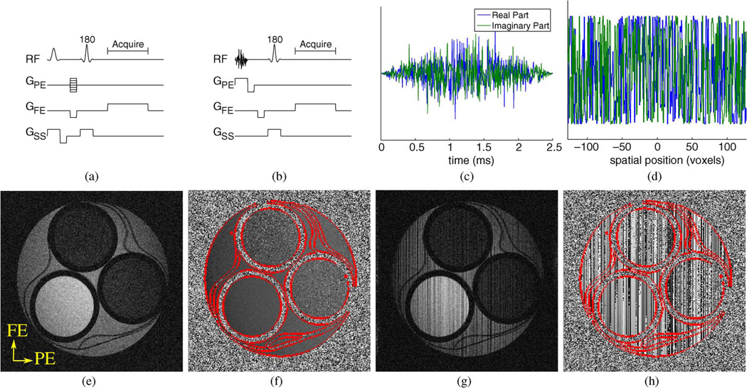
To make random encoding more practical, we consider a modification based on the conventional spin-warp imaging sequence shown in Fig. 1(a). In spin-warp imaging, each excitation is followed by phase encoding, and a full frequency-encoded line passing through the center of k-space is read out after the signal is refocused by a 180° pulse. In this manner, Cartesian coverage of k-space is obtained, with the total number of excitations given by the total number of phase encodings.

Fig. 1.

(a) The conventional Fourier-encoded spin-warp sequence, and (b) the proposed 1D random-encoding sequence. G_PE, G_FE, and G_SS represent the gradients along the phase encoding, frequency encoding, and slice select dimensions, respectively. Also shown are (c) a typical random-encoding RF pulse and (d) its corresponding excitation profile. The impact of random-encoding is depicted with real experimental data in (e)–(h). The (e) magnitude and (f) phase of a phantom acquired with standard excitation and full Fourier encoding, as compared to the (g) magnitude and (h) phase of the same phantom acquired with random-encoding excitation and full Fourier encoding. The frequency encoding (FE) and phase encoding (PE) directions for these images are labeled in (e).

Our proposed modification of conventional spin-warp imaging replaces phase encoding by random 1D spatially-selective excitation, and is shown in Fig. 1(b). In particular, assuming that x is the phase encoding dimension and y is the frequency encoding dimension, we use

$$w_m(x,y)={\displaystyle \sum _{q=-Q/2}^{Q/2-1}}{\gamma }_{\mathit{\text{qm}}}{\displaystyle \prod }(x-q)$$ (11)

where γ_qm are Gaussian distributed as before, and w_m(x, y) is the same for all samples from the same excitation.

The RF pulses used to achieve the 1D excitation profiles from (11) are designed using the small tip-angle approximation [48], such that the excitation RF pulse waveform can be generated by taking the Fourier transform of the desired 1D excitation profile. An example RF pulse and the corresponding excitation profile are shown in Fig. 1(c) and (d).

This form of random encoding requires the use of RF pulses for both spatial encoding and slice selection. Given the limitations of current multidimensional excitation technology, this necessitates the use of multiple pulses in practice. This limitation is common to other 2D non-Fourier encoding schemes that use spatially-selective excitation (e.g., [43], [46]), though can be overcome if the RF encoding is applied only along the third dimension of a 3D experiment (e.g., [8], [45]). In addition, the use of varying excitation angles can complicate steady-state behavior [49]. This issue is also present for other similar non-Fourier encoding techniques, and is generally overcome by using small flip angles and relatively long repetition times [50]. Use of random encoding outside of this regime can mean that data acquisition is nonlinear and no longer accurately modeled by (7). The use of nonlinear random encoding does not fall within the scope of conventional CS or this paper; however, preliminary empirical investigations of nonlinear random encoding can be found in [39], in which ℓ₁ regularization ℓ₁ is used in the context of a parametric nonlinear signal model.

III. Evaluation And Discussion

Experiments and simulations were performed to investigate the properties of random encoding for CS-MRI. In all cases, we compared three different data acquisition schemes with a fixed number M of data samples.

• Random Encoding. The proposed practical random encoding scheme with 1D spatially-selective RF excitations, as described in Section II-B.

• Fourier Encoding 1 (FE1). This scheme uses the standard spin-warp sequence from Fig. 1(a). The phase encoding locations are evenly-spaced at the Nyquist rate, and cover the low-frequency portion of k-space.

• Fourier Encoding 2 (FE2). Similar to FE1, FE2 makes use of the standard spin-warp sequence. However, the phase-encoding locations are chosen randomly from the Nyquist grid according to a discretized Gaussian distribution centered at low-frequency k-space. This type of variable-density random sampling scheme performs empirically better than sampling k-space uniformly at random, and is consistent with both the prior knowledge that the typical images seen in MRI have energy concentrated at low-frequencies and the existing CS-MRI literature [8], [51].

A. Experiments

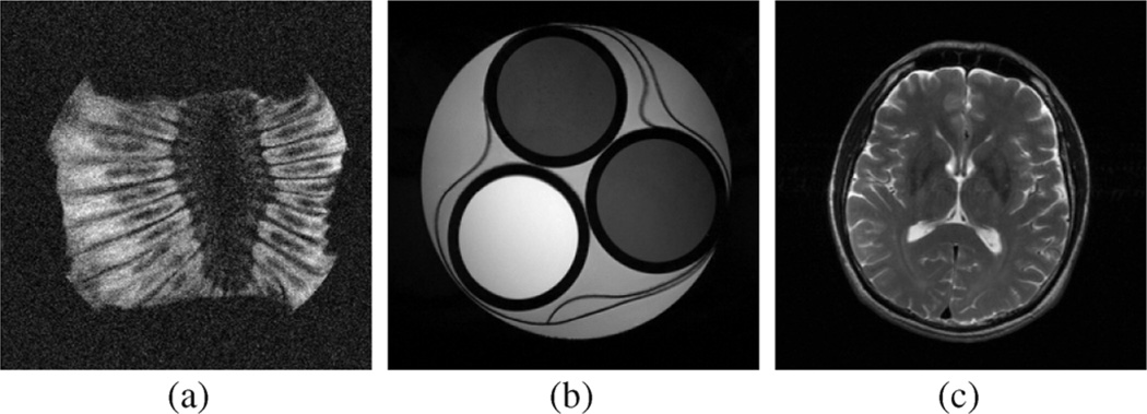
The three different encoding schemes were implemented on a 14.1 T magnet system (Oxford Instruments, Abingdon, U.K.) interfaced with a Unity console (Varian, Palo Alto, CA). The flip angle for FE1 and FE2 encoding and the root mean square flip angle for random encoding was 50°, with an RF pulse duration of 2.5 ms. The field of view was 3 cm × 3 cm, the slice thickness was 4 mm, the sequence timing parameters were TE/TR = 26/500 ms, and the bandwidth of the random encoding pulses was approximately 200 kHz. Data was collected for reconstruction on a 256 × 256 voxel grid using two different test objects: a compartmental phantom and a section of kiwi fruit. The estimated SNR³ for full 256 × 256 Fourier encoded data was approximately 4 for the compartmental phantom image [shown in Fig. 1(e)], and approximately 6 for the kiwi fruit image [shown in Fig. 2(a)].

Fig. 2.

Fully Fourier-encoded images of the section of kiwi fruit from a real experiment is shown in (a). High-SNR images of the compartmental phantom and the brain image used for simulations are shown in (b) and (c), respectively.

Due to nonideal experimental conditions (e.g., B₀ and B₁ inhomogeneity at this field strength), the experimentally achieved excitation profiles used for random encoding did not match exactly with the designed profiles. As such, the excitation profile of each pulse was calibrated using prescans. Specifically, a fully-Fourier encoded image ρ_cal(x, y) was acquired for each of the spatially-selective excitation pulses [one such image is shown in Fig. 1(g) and (h)]. From these images, the γ_qm parameters for each excitation profile [cf. (11)] were derived by solving the least squares problem

$${\widehat{\gamma }}_{\mathit{\text{qm}}}=\text{arg}\underset{{\gamma }_{\mathit{\text{qm}}}}{\text{min}}{\displaystyle \sum _{p=-P/2}^{P/2-1}}{|{\gamma }_{\mathit{\text{qm}}}{\rho }_{\text{ref}}(q,p)-{\rho }_{\text{cal}}(q,p)|}^2$$ (12)

where ρ_ref(x, y)is an image acquired using traditional excitation pulses. This calibration procedure is somewhat coarse, since we ignore any potential excitation inhomogeneity along the frequency-encoding direction, though this choice leads to improved noise robustness compared to voxel-by-voxel estimation. In addition, while acquiring data for this calibration procedure is time consuming, the procedure could be simplified through direct mapping of the B₁ transmit field and more accurate modeling of the excitation physics.

CS reconstructions were performed by solving

$$\text{minimizeTV}({\widehat{\mathrm{\rho }}}_{\text{CS}})\text{subject to}{\Vert \mathbf{E}{\widehat{\mathrm{\rho }}}_{\text{CS}}-\mathbf{d}\Vert }_{{\ell }_2}^2\le {\epsilon }^2$$ (13)

where ε was chosen according to an estimate of the expected data error due to noise (i.e.,ε² = Mσ², where σ² is the estimated noise variance and M is the number of measurements), and TV(ρ) is the total variation (TV) [52] cost functional that penalizes ℓ₁ the norm of the magnitude of the image gradient. Penalizing the image gradient is very common for CS reconstruction of MR images (e.g., [8], [10], [15], [16]), since medical images are often approximately piecewise smooth, though it should be noted that the magnitude of the image gradient is a nonlinear transformation of the image and cannot be represented by a matrix Ψ. Reconstructions were obtained using a version of Nesterov’s algorithm as described in [53], with minor modifications to handle complex images. The specific implementation of the algorithm described in [53] directly solves (13) for the special case when E is a submatrix of a unitary transform. While the encoding matrix has this property with Cartesian Fourier encoding, it does not have this property for random encoding. As a result, we use Nesterov’s algorithm to solve the Lagrangian form of (13) when reconstructing data acquired with random encoding [53]

$$\text{minimizeTV}({\widehat{\mathrm{\rho }}}_{\text{CS}})+\lambda \left({\Vert \mathbf{E}{\widehat{\mathrm{\rho }}}_{\text{CS}}-\mathbf{d}\Vert }_{{\ell }_2}^2-{\epsilon }^2\right)$$ (14)

where λ is a Lagrange multiplier that is adjusted to satisfy the Karush–Kuhn–Tucker conditions for (13). In most practical cases of interest (i.e., when ‖d‖_ℓ2 > ε), λ should be chosen such that ${\Vert \mathbf{E}{\widehat{\rho }}_{\text{CS}}-\mathbf{d}\Vert }_{{\ell }_2}^2={\epsilon }^2$, which will ensure that the solution to (14) is equivalent to the solution of (13) [53]. Selection of λ to satisfy this condition is straightforward, since the data-fidelity of the solution to (14) is monotonically decreasing with increasing λ. Note that the E matrix associated with random encoding has very similar structure to the encoding matrix used in SENSE parallel imaging reconstruction [47], except that RF excitation profiles are used in place of receiver coil sensitivity profiles. As a result, multiplication with E and its conjugate transpose can be performed efficiently using fast Fourier transforms [47], and these techniques were used to accelerate computations in the present context.

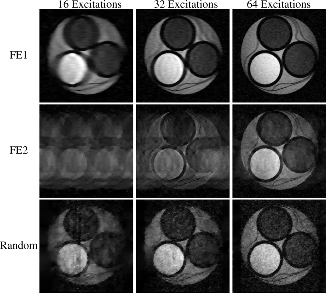
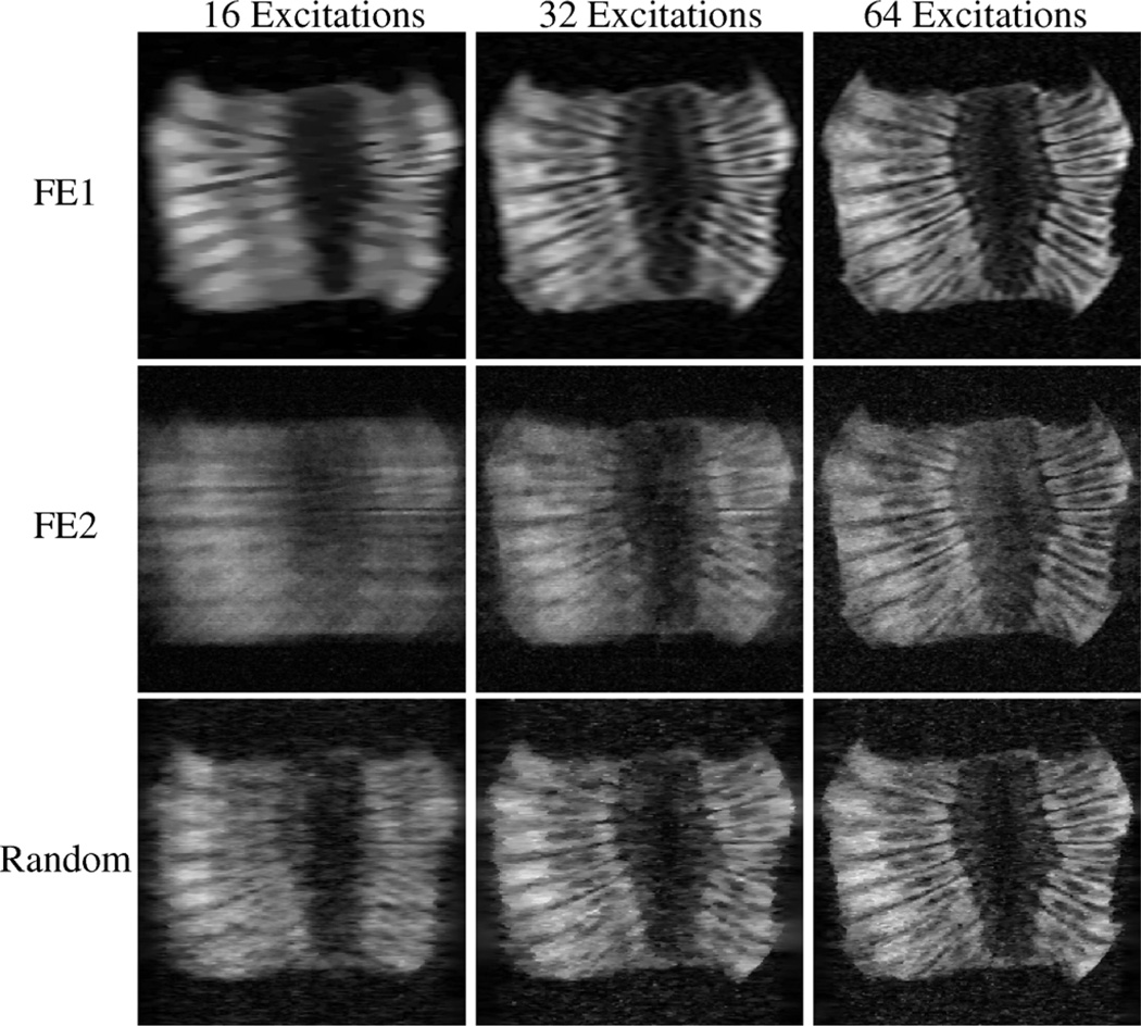
Reconstructions from the experiment with the low-SNR compartmental phantom and the higher-SNR kiwi fruit are shown in Figs. 3 and 4, respectively. With FE1, the CS reconstruction looks very similar to what would be obtained from conventional zero-padded reconstruction of low-frequency data, with accurate contrast information for low-resolution features, but also with significant blurring and distortion of the object geometry. With FE2, contrast is less accurate than with FE1, though the high-resolution image features are reconstructed better with FE2 than with FE1 with sufficient data. Results using random encoding indicate that it is possible to use this new scheme for CS-MRI, and that random encoding yields reconstructions with different characteristics than what are obtained with more traditional Fourier-based schemes. The figures suggest that random RF excitation can encode both high- and low-resolution image structures reasonably well, leading to a more-balanced trade-off between contrast and resolution. Notably, some of the high-resolution image geometry is visible using random encoding with only 16 excitations (e.g., the geometry of the circular compartments in Fig. 3 and some of the fine edge structures in Fig. 4), while these features are significantly distorted with the other two schemes.

Fig. 3.

CS-MRI reconstructions from real experimental data from the compartmental phantom. Each row represents a different encoding scheme, while each column represents a different amount of measured data. These reconstructions demonstrate that CS-MRI with random encoding is feasible, and has different characteristics than either FE1 (which samples low-frequency k-space) or FE2 (which uses randomized k-space phase-encoding locations).

Fig. 4.

CS-MRI reconstructions of real experimental data from the section of kiwi fruit. Each row represents a different encoding scheme, while each column represents a different amount of measured data. As before, random encoding enables visualization of both low- and high-resolution image features with very limited data.

Similar to FE1 and FE2, reconstructions with random encoding become more accurate with increasing data. However, different from reconstructions with highly-undersampled FE1 and FE2 acquisitions (which can demonstrate significant geometry and/or large-scale contrast errors), the artifacts resulting from very limited random encoding data are more similar to the artifacts that might be observed from image compression (i.e., the loss of contrast for smaller image features). In addition, we should note that random encoding reconstructions also contain some artifacts that are not found in FE1 or FE2 reconstructions, and which could be attributed to noise, non-Gaussian excitation profiles, and/or errors in the calibration of the excitation profiles.

B. High-SNR Simulations

1) Compartmental Phantom

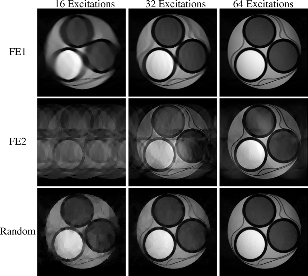
Simulations were also performed to illustrate performance when noise perturbations and calibration errors are minimal. The first set of simulations used a high-SNR image of the compartmental phantom as a gold standard, used nominal Gaussian excitation profiles, and incorporated simulated noise that was significantly weaker than that observed with the experimental data [the SNR was 80 with respect to the image from full 256 × 256 Fourier encoded data, which is shown in Fig. 2(b)]. Figs. 5 and 6 show representative results from these simulations. The improved SNR and nominal excitation profiles have led to improved reconstruction quality for all schemes, though random encoding now demonstrates a more distinct advantage relative to the others. The relative errors are shown in Table I, where relative error is defined as

$$\text{Relative Error}=\frac{{\Vert \mathrm{\rho }-{\widehat{\mathrm{\rho }}}_{\text{cs}}\Vert }_{{\ell }_2}}{{\Vert \mathrm{\rho }\Vert }_{{\ell }_2}}$$ (15)

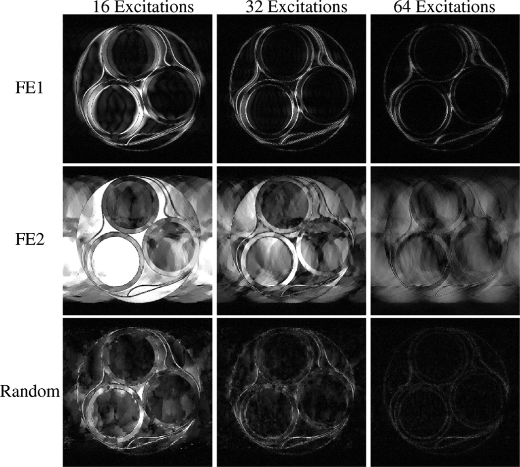
and serves as a measure of similarity between the reconstructed image ρ̂_cs and the gold-standard image ρ. For these simulations, random encoding outperformed both FE1 and FE2 in relative error at all investigated undersampling levels. As with the experimental results, it was observed that the distribution of errors with random encoding CS-MRI reconstructions was more evenly distributed between low- and high-resolution features than with FE1 or FE2.

Fig. 5.

CS-MRI reconstructions from high-SNR simulations of the compartmental phantom. Each row represents a different encoding scheme, while each column represents a different amount of measured data. Relative to the experimental data, the improved SNR leads to better reconstructions for all encoding schemes. Reasonably accurate reconstruction was obtained using random encoding with only 32 excitations, while the Fourier encoding schemes required more data to achieve the same accuracy.

Fig. 6.

Error images (i.e., the difference between the gold standard and the reconstruction) corresponding to the high-SNR simulation results shown in Fig. 5. Each row represents a different encoding scheme, while each column represents a different amount of measured data. The error images have been scaled up by a factor of 3 for improved visualization.

TABLE I.

Relative Reconstruction Errors for the High-SNR Simulations Using the Compartmental Phantom

	Relative Error
Encoding Scheme	16 Excitations	32 Excitations	64 Excitations
FE1	0.249	0.149	0.086
FE2	0.713	0.394	0.265
Random	0.245	0.121	0.053
Random (real profiles)	0.252	0.133	0.065
Random (2D profiles)	0.127	0.079	0.048

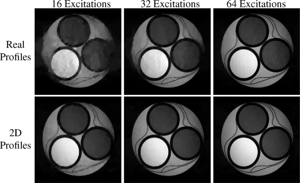
Fig. 7 shows results from additional random encoding simulations (relative errors for these are also shown in Table I), where the excitation profiles were chosen to either be the empirically measured excitation profiles from the real experiment (“real profiles”) or ideal 2D profiles (“2D profiles”) as in (10). As in the previous simulations, the SNR with respect to fully-encoded Fourier data was 80, and one frequency encoding line was acquired per excitation. The results with the real profiles are very similar to the results with the nominal profiles, and illustrate that it is not necessary to have perfectly white Gaussian γ_qm excitation profile parameters to have good reconstruction results. The results using 2D profiles in Fig. 7 demonstrate significantly improved performance relative to 1D random encoding, and indicate that even better results could be achieved if high-resolution multidimensional RF excitation techniques become more practical.

Fig. 7.

CS-MRI reconstructions from high-SNR random encoding simulations of the compartmental phantom. The top row shows results using the calibrated excitation profiles from a real experiment, while the bottom row shows results using random 2D excitation profiles.

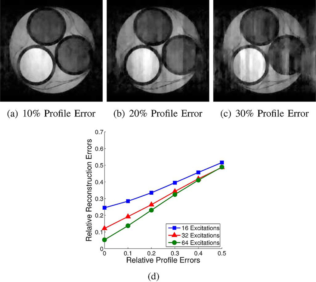
The quality of reconstructed images using random encoding can also be affected by errors in the encoding matrix E due to miscalibration of the RF excitation profiles. Theoretical analysis of (3) when E contains errors has been presented recently by Herman and Strohmer [54]. These results indicate that stable and accurate CS reconstructions can still be guaranteed with a noisy E, under the assumptions that the true measurement matrix satisfies an appropriate RIP condition and that the magnitude of the perturbation is not too large. In particular, the theoretical analysis and numerical simulations in [54] suggest that the stability of ρ̂_cs should scale linearly with the amount of perturbation to the system matrix. Simulation studies were performed to examine the effects of RF profile miscalibration. High-SNR data was simulated using standard 1D random encoding with nominal Gaussian RF profiles, and the RF profile parameters γ_qm used for reconstruction were perturbed by Gaussian noise. Results of these simulations are shown in Fig. 8. These results suggest a linear relationship between reconstruction error and calibration error, as might be expected based on the theoretical analysis [54].

Fig. 8.

Simulated random-encoding reconstruction results in the presence of miscalibration of the RF excitation profiles. (a)–(c) Representative reconstructions from 32 excitations in the presence of increasing levels of calibration error. (d) The total reconstruction error (shown averaged over five realizations) is observed to grow linearly with respect to the calibration error.

2) Brain Phantom

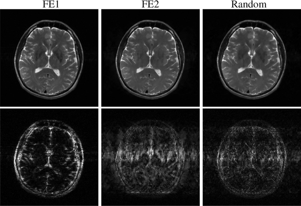
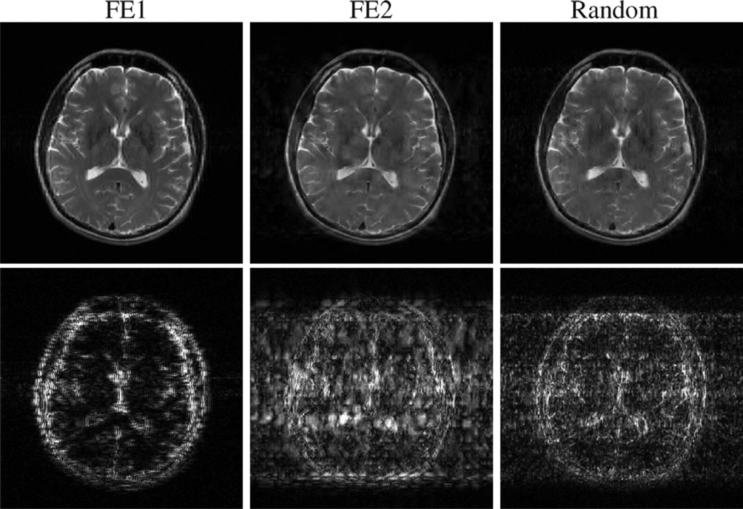
High-SNR simulations were also performed with the brain image shown in Fig. 2(c). The simulations in this case had the same noise level as the high-SNR compartmental phantom simulations. Representative reconstructions from 96 excitations and either TV or a wavelet (Daubechies-4) sparsifying transform are shown in Figs. 9 and 10. Representative relative reconstruction errors for a range of undersampling levels are listed in Table II.

Fig. 9.

Simulated CS-MRI reconstructions of the compressible brain image from 96 excitations, with a TV penalty. The top row shows the reconstructions themselves, while the bottom row shows the differences (scaled up by a factor of 6) between the reconstructions and the gold standard.

Fig. 10.

Simulated CS-MRI reconstructions of the compressible brain image from 96 excitations, with a Daubechies-4 wavelet penalty. The top row shows the reconstructions themselves, while the bottom row shows the differences (scaled up by a factor of 6) between the reconstructions and the gold standard.

TABLE II.

Relative Reconstruction Errors for the High-SNR Simulations Using the Brain Image

	Relative Error
Encoding Scheme (Sparsifying Transform)	64 Excitations	96 Excitations	128 Excitations
FE1 (TV)	0.179	0.119	0.076
FE2 (TV)	0.184	0.113	0.074
Random (TV)	0.154	0.090	0.055
FE1 (wavelet)	0.228	0.154	0.117
FE2 (wavelet)	0.330	0.191	0.133
Random (wavelet)	0.251	0.158	0.099

The brain image has lower compressibility than the compartmental phantom, and is thus more challenging for CS-MRI and required a larger amount of data for accurate reconstruction. In addition, the performance advantage (in terms of relative error) of random encoding relative to FE1 and FE2 was less substantial than it was with the compartmental phantom simulations. This was particularly true using the wavelet-based constraint, which was significantly less-effective than the TV constraint for all encoding schemes. However, the spatial distributions of error for both TV and wavelet sparsity are still consistent with what was observed previously. In particular, the errors for FE1 encoding are concentrated around the high-resolution features of the image, while there are significant contrast errors for low-resolution image features with FE2 encoding. The distribution of errors with random encoding is intermediate between the FE1 and FE2 cases, with the errors somewhat more uniformly distributed between low- and high-resolution image features. These characteristics have been observed consistently in both simulations and experiments, and are important to note when choosing an encoding scheme for a particular imaging scenario, since different features will have more or less importance depending on the application.

C. Monte Carlo Simulations

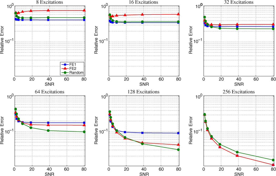
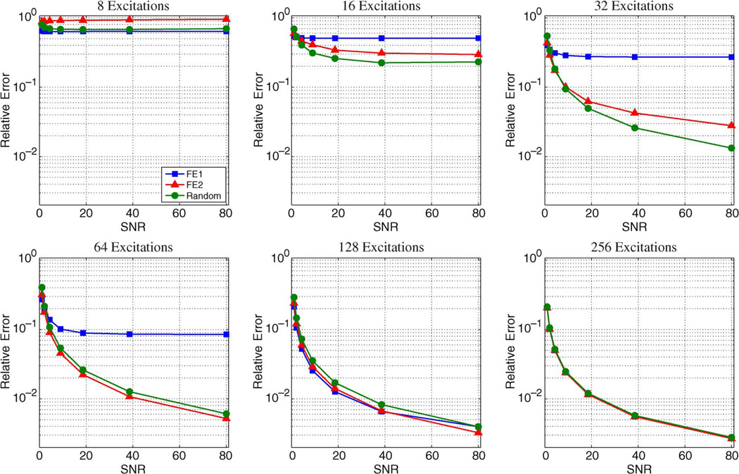
Monte Carlo simulations were also performed to study the reconstruction and noise properties of random encoding relative to FE1 and FE2. In these simulations, reconstructions were performed using an image with a sparse gradient (the Shepp–Logan phantom) and an image with a compressible gradient [the MR brain image shown in Fig. 2(c)]. Simulations were performed 50 times for each combination of six data undersampling levels (8, 16, 32, 64, 128, and 256 excitations), the three different encoding schemes (FE1, FE2, and random encoding), and seven different noise levels (SNRs ranging from 1 to 80 with respect to full 256 × 256 Fourier encoding). The random elements of the simulation (i.e., the sampling locations for FE2 encoding, the excitation profiles for random encoding, and the noise) were different for each trial. To improve the computational speed for these 12 600 reconstructions, each reconstruction made use of a simplified 1D TV penalty that only penalized the ℓ₁ norm of the difference between adjacent voxel values along the phase-encoding dimension. Since the frequency encoding dimension was fully sampled, this modified TV penalty means that the optimal two-dimensional 256 × 256 CS reconstruction could be performed using 256 independent smaller 1D CS reconstructions, one for each line of the image. This simplification allows reconstructions to be performed much more rapidly than if standard TV was used, and additionally means that the matrix E for each subproblem has the ideal “universal” distribution. To solve these 1D CS problems, we used the CVX software package by Grant, Boyd, and Ye (http://www.stanford.edu/~boyd/cvx/).

Results from the Monte Carlo simulations using the brain image and the sparse Shepp–Logan phantom are shown in Figs. 11 and 12, respectively. Images are generally more compressible using a 2D transform rather than a 1D transform, leading to slightly lower performance for these simulations compared to those in the previous subsection. However, the relative performance characteristics of the different encoding schemes with 1D sparsity constraints are consistent with the behavior observed with 2D constraints. For both images in the Monte Carlo simulations, the relative error decreases as the amount of acquired data increases, and FE1 encoding was generally superior to both FE2 and random encoding in cases with very limited data or with high levels of noise. FE2 encoding consistently outperforms FE1 encoding with high-SNR data when the number of measurements is large. Random encoding can outperform both FE1 and FE2 encoding, though this only occurs with high-SNR data, and the advantage of random encoding over the Fourier-based schemes disappears as the number of measurements M becomes comparable to the number of voxels N. One way of understanding this phenomenon is to consider the case of fully-sampled data (i.e., M = N) with standard reconstruction, where the reconstructed image is obtained by ρ̂ = E⁻¹d. In this case, the discrete Fourier transform (DFT) matrix is unitary, which means that the noise in the data will not be amplified by E⁻¹. In contrast, fully-sampled random encoding matrices will generally have worse condition numbers than the DFT matrix [55], resulting in more significant noise amplification.

Fig. 11.

Plots showing the median relative error as a function of SNR from the Monte Carlo simulations with a brain image. In all cases, the relative error decreases as the amount of acquired data increases. FE1 encoding was generally superior in cases with very limited data or with high levels of noise. However, for moderate noise and sufficient data acquisition, random encoding performed better than the other two schemes, and FE2 outperforms FE1. For fully-encoded data, the SNR efficiency of the Fourier schemes allows them to dominate the random encoding scheme.

Fig. 12.

Plots showing the median relative error as a function of SNR from the Monte Carlo simulations with the Shepp–Logan phantom. The trends are similar to those observed for the compressible brain image, though for the same number of measurements, smaller relative error is generally achieved with this sparse image. Notably, the regime for which random encoding outperforms the Fourier-based schemes is different than it was with the brain image.

Similar Monte Carlo simulations imposing a 1–D wavelet-based sparsity constraint showed similar characteristics to those observed with the 1D TV constraint, and are not shown due to space limitations. Notably, the regimes for which random encoding outperforms the Fourier-based schemes (in terms of relative error) are different for the Shepp–Logan phantom compared to the brain image, and are also different for different sparsifying transforms (i.e., the 1D TV and wavelet transforms and the 2D transforms considered in the previous subsection). This further suggests that the choice between the use of random encoding versus a Fourier encoding scheme should be made carefully based on the constraints of each application.

D. Performance Guarantees

The use of random encoding in this work was motivated by the desire to improve restricted isometry constants and improve the theoretical characterization of CS-MRI reconstruction. As mentioned in the introduction, it is generally computationally infeasible to compute the restricted isometry constants. However, it is relatively straightforward to calculate the δ₁ restricted isometry constant for a matrix Φ using (5) with

$${\alpha }_1=\underset{i}{\text{min}}{\Vert {\mathrm{\varphi }}_i\Vert }_{{\ell }_2}^2\text{and}{\beta }_1=\underset{i}{\text{max}}{\Vert {\mathrm{\varphi }}_i\Vert }_{{\ell }_2}^2$$ (16)

where the vectors ϕ_i are the columns of Φ.

Besides RIPs, there are also incoherence conditions on Φ that can guarantee good CS performance [23]–[25]. While these incoherence-based guarantees are generally weaker than RIP-based guarantees, they have been used previously in the design of CS-MRI encoding schemes [8] and in other contexts [56]. For example, Lustig et al. [8] suggested that the maximum of the transform point spread function (TPSF) be used to characterize the incoherence of a sampling scheme, with more incoherent sampling schemes characterized as better for CS reconstruction. The TPSF has the form

$$\text{TPSF}\{i;j\}=\frac{{\mathrm{\varphi }}_j^H{\mathrm{\varphi }}_i}{{\Vert {\mathrm{\varphi }}_i\Vert }_{{\ell }_2}{\Vert {\mathrm{\varphi }}_j\Vert }_{{\ell }_2}}$$ (17)

and is somewhat representative of the level of ambiguity between the ith and jth transform coefficients. Ideally, the TPSF should be small when i ≠ j. The maximum of the TPSF is equal to the mutual incoherence μ

$$\mu =\underset{i\ne j}{\text{max}}|\text{TPSF}\{i;j\}|$$ (18)

which can be used to generate another set of CS performance guarantees [23], [24], [57]. For example, if ‖c‖_ℓ0 < (1/4)(1/μ + 1) and if the columns of Φ are normalized to unit length, then the solution to (3) is guaranteed to satisfy (see [24, Th. 3.1])

$${\Vert {\widehat{\mathbf{c}}}_{\text{cs}}-\mathbf{c}\Vert }_{{\ell }_2}^2\le \frac{4{\epsilon }^2}{1-\mu (4{\Vert \mathbf{c}\Vert }_{{\ell }_0}-1)}$$ (19)

where ‖x‖ℓ₀ is defined as the number of nonzero entries of x

Table III shows representative values of δ₁ and μ for the three encoding schemes we have considered and using a Ψ matrix corresponding to a Daubechies-4 wavelet transform. Values are shown for reconstruction of both a 256 × 256 image and a 128 × 128 image. For the 256 × 256 case, both δ₁ and μ are smaller for random encoding than for FE1 and FE2. However, it is also important to note that δ₁ is never less than 0.307 for any encoding scheme, and only is only less than 0.4734 for random encoding with 64 frequency encoding lines. Since it is always true that when δ_t ≥ δ_s, t ≥ s this implies that the current RIP-based guarantees for CS performance cannot be applied to the other measurement matrices, even for signals that have only one nonzero entry. Similar to what was observed with δ₁, μ is also smallest for random encoding at this image resolution. However, the characterization given by (19) can only be applied for nonzero vectors c when μ < 1/3, so the observed μ values give no useful guarantees for any of the encoding schemes. Despite this, CS empirically works much better than what the theoretical bounds might suggest, and it is promising that random encoding yields the smallest δ₁ and μ values.

TABLE III.

Representative δ₁ Restricted Isometry Constants and Mutual Incoherence μ Values for Different Encoding Schemes, Different Amounts of Acquired Data, and Different Image Grid Sizes. Calculations Were Performed Using a Daubechies-4 Wavelet Basis

		δ1		μ
Grid Size	Encoding Scheme	32 Excitations	64 Excitations	32 Excitations	64 Excitations
256×256	FE1	0.9996	0.9876	0.9005	0.7833
	FE2	0.7636	0.7093	0.7147	0.6665
	Random	0.5070	0.3567	0.5594	0.4179
128×128	FE1	0.9874	0.7706	0.7840	0.7425
	FE2	0.2655	0.0847	0.6201	0.3612
	Random	0.4592	0.4129	0.5619	0.3635

It is also important to note that the good theoretical properties for “universal” encoding are somewhat dependent on the problem size, with a higher probability of good RIPs as M and N grow large [4]. We have observed that the superiority of the μ and δ₁ values for random encoding is also dependent on the problem size. For example, with a 128 × 128 image, we have observed that FE2 has consistently better δ₁ values relative to random encoding, which is opposite from the behavior observed with 256 × 256 images. However, it is observed that μ does not follow the same trend as for this 128 × 128 case, and that μ can still be smaller for random encoding than for FE2 (cf. Table III).

E. Non-Cartesian Acquisitions and Multidimensional Undersampling

For both Fourier and random encoding, we have focused on 2D Cartesian k-space sampling patterns with undersampling along a single dimension to keep the discussion as short and simple as possible. In practice, however, several CS-MRI studies have shown good results when using non-Cartesian Fourier sampling patterns and/or multidimensional undersampling schemes (e.g., [8]–[20]). We note that non-Cartesian and multidimensionally-undersampled forms of random encoding are also possible, though there are several ways of implementing such schemes. For example, a naive approach to non-Cartesian random encoding would be to maintain the same 1D spatially-selective excitation scheme as in Section II-B, but replace standard frequency-encoding with a non-Cartesian readout. A more complicated implementation could change the orientation of RF encoding for each excitation pulse in combination with a non-Cartesian readout. Preliminary simulations using both of these schemes with Fourier encoding along radial lines indicate further performance improvements [34], though a detailed investigation of these and other multidimensional encoding schemes is left for future work.

IV. Conclusions

This work introduces a random encoding scheme for CS-MRI, replacing traditional phase encoding with RF encoding using randomized excitation profiles. This random scheme is conceptually similar to the “universal” encoding schemes suggested by the CS literature, and simulations and experiments reveal that it has the potential to outperform Fourier-based schemes in certain high-SNR scenarios. However, our study also indicates that the random encoding scheme fails to satisfy the theoretical sufficient conditions for stable and accurate CS reconstruction in many scenarios of interest. Therefore, there is still no general theoretical performance guarantee for CS-MRI, with or without random encoding. As a result, the practical utility of CS methodology for MRI should be evaluated carefully for each application.

References

- 1.Candès EJ, Romberg J, Tao T. Robust uncertainty principles: Exact signal reconstruction from highly incomplete frequency information. IEEE Trans. Inf. Theory. 2006 Feb.vol. 52(no. 2):489–509. [Google Scholar]
- 2.Donoho DL. Compressed sensing. IEEE Trans. Inf. Theory. 2006 Apr.vol. 52(no. 4):1289–1306. [Google Scholar]
- 3.Candès E, Tao T. Near optimal signal recovery from random projections: Universal encoding strategies. IEEE Trans. Inf. Theory. 2006 Dec.vol. 52(no. 12):5406–5425. [Google Scholar]
- 4.Candès E, Tao T. Decoding by linear programming. IEEE Trans. Inf. Theory. 2005 Dec.vol. 51(no. 12):4203–4215. [Google Scholar]
- 5.Candès EJ, Romberg JK, Tao T. Stable signal recovery from incomplete and inaccurate measurements. Comm. Pure Appl. Math. 2006;vol. 59:1207–1223. [Google Scholar]
- 6.Feng P, Bresler Y. Spectrum-blind minimum-rate sampling and reconstruction of multiband signals; Proc. IEEE Int. Conf. Acoust., Speech, Signal Process; 1996. pp. 1688–1691. [Google Scholar]
- 7.Venkataramani R, Bresler Y. Further results on spectrum blind sampling of 2D signals; Proc. IEEE Int. Conf. Image Process; 1998. pp. 752–756. [Google Scholar]
- 8.Lustig M, Donoho D, Pauly JM. Sparse MRI: The application of compressed sensing for rapid MR imaging. Magn. Reson. Med. 2007;vol. 58:1182–1195. doi: 10.1002/mrm.21391. [DOI] [PubMed] [Google Scholar]
- 9.Lustig M, Santos JM, Donoho DL, Pauly JM. k-t SPARSE: High frame rate dynamic MRI exploiting spatio-temporal sparsity. Proc. Int. Soc. Magn. Reson. Med. 2006:2420. [Google Scholar]
- 10.Block KT, Uecker M, Frahm J. Undersampled radial MRI with multiple coils. iterative image reconstruction using a total variation constraint. Magn. Reson. Med. 2007;vol. 57:1086–1098. doi: 10.1002/mrm.21236. [DOI] [PubMed] [Google Scholar]
- 11.Jung H, Ye JC, Kim EY. Improved k − t BLAST and k − t SENSE using FOCUSS. Phys. Med. Biol. 2007;vol. 52:3201–3226. doi: 10.1088/0031-9155/52/11/018. [DOI] [PubMed] [Google Scholar]
- 12.Ye JC, Tak S, Han Y, Park HW. Projection reconstruction MR imaging using FOCUSS. Magn. Reson. Med. 2007;vol. 57:764–775. doi: 10.1002/mrm.21202. [DOI] [PubMed] [Google Scholar]
- 13.Gamper U, Boesiger P, Kozerke S. Compressed sensing in dynamic MRI. Magn. Reson. Med. 2008;vol. 59:365–373. doi: 10.1002/mrm.21477. [DOI] [PubMed] [Google Scholar]
- 14.Hu S, Lustig M, Chen AP, Crane J, Kerr A, Kelley DAC, Hurd R, Kurhanewicz J, Nelson SJ, Pauly JM, Vigneron DB. Compressed sensing for resolution enhancement of hyperpolarized 13C flyback 3D-MRSI. J. Magn. Reson. 2008;vol. 192:258–264. doi: 10.1016/j.jmr.2008.03.003. [DOI] [PMC free article] [PubMed] [Google Scholar]
- 15.Trzasko J, Manduca A. Highly undersampled magnetic resonance image reconstruction via homotopic ℓ0-minimization. IEEE Trans. Med. Imag. 2009 Jan.vol. 28(no. 1):106–121. doi: 10.1109/TMI.2008.927346. [DOI] [PubMed] [Google Scholar]
- 16.Kim Y-C, Narayanan SS, Nayak KS. Accelerated three-dimensional upper airway MRI using compressed sensing. Magn. Reson. Med. 2009;vol. 61:1434–1440. doi: 10.1002/mrm.21953. [DOI] [PMC free article] [PubMed] [Google Scholar]
- 17.Schirra CO, Weiss S, Krueger S, Pedersen SF, Razavi R, Schaeffter T, Kozerke S. Toward true 3D visualization of active catheters using compressed sensing. Magn. Reson. Med. 2009;vol. 62:341–347. doi: 10.1002/mrm.22001. [DOI] [PubMed] [Google Scholar]
- 18.Liang D, Liu B, Wang JJ, Ying L. Accelerating SENSE using compressed sensing. Magn. Reson. Med. 2009;vol. 62:1574–1584. doi: 10.1002/mrm.22161. [DOI] [PubMed] [Google Scholar]
- 19.Seeger M, Nickisch H, Pohmann R, Schölkopf B. Optimization of k-space trajectories for compressed sensing by Bayesian experimental design. Magn. Reson. Med. 2010;vol. 63:116–126. doi: 10.1002/mrm.22180. [DOI] [PubMed] [Google Scholar]
- 20.Ajraoui S, Lee KJ, Deppe MH, Parnell SR, Parra-Robles J, Wild JM. Compressed sensing in hyperpolarized 3He lung MRI. Magn. Reson. Med. 2010;vol. 63:1059–1069. doi: 10.1002/mrm.22302. [DOI] [PubMed] [Google Scholar]
- 21.Candès EJ. The restricted isometry property and its implications for compressed sensing. C. R. Acad. Sci. Paris, Ser. I. 2008;vol. 346:589–592. [Google Scholar]
- 22.Davies ME, Gribonval R. Restricted isometry constants where ℓp sparse recovery can fail for 0 < p ≤ 1. IEEE Trans. Inf. Theory. 2009;vol. 55:2203–2214. [Google Scholar]
- 23.Donoho DL, Elad M. Optimally sparse representation in general (nonorthogonal) dictionaries via ℓ1 minimization. Proc. Natl. Acad. Sci. USA. 2003;vol. 100:2197–2202. doi: 10.1073/pnas.0437847100. [DOI] [PMC free article] [PubMed] [Google Scholar]
- 24.Donoho DL, Elad M, Temlyakov VN. Stable recovery of sparse overcomplete representations in the presence of noise. IEEE Trans. Inf. Theory. 2006 Jan.vol. 52(no. 1):6–18. [Google Scholar]
- 25.Candès E, Romberg J. Sparsity and incoherence in compressive sampling. Inverse Probl. 2007;vol. 23:969–985. [Google Scholar]
- 26.Cohen A, Dahmen W, DeVore R. Compressed sensing and best k-term approximation. J. Am. Math. Soc. 2009;vol. 22:211–231. [Google Scholar]
- 27.Donoho DL, Huo X. Uncertainty principles and ideal atomic decomposition. IEEE Trans. Inf. Theory. 2001 Nov.vol. 47(no. 7):2845–2862. [Google Scholar]
- 28.Gribonval R, Nielsen M. Sparse representations in unions of bases. IEEE Trans. Inf. Theory. 2003 Dec.vol. 49(no. 12):3320–3325. [Google Scholar]
- 29.Foucart S. A note on guaranteed sparse recovery via ℓ1-minimization. Appl. Comput. Harmon. Anal. 2009;vol. 29:97–103. [Google Scholar]
- 30.Cai TT, Wang L, Xu G. New bounds for restricted isometry constants. IEEE Trans. Inf. Theory. 2010 Sep.vol. 56(no. 9):4388–4394. [Google Scholar]
- 31.Rudelson M, Vershynin R. On sparse reconstruction from Fourier and Gaussian measurements. Comm. Pure Appl. Math. 2008;vol. 61:1025–1045. [Google Scholar]
- 32.Donoho DL, Tanner J. Exponential bounds implying construction of compressed sensing matrices, error-correcting codes, and neighborly polytopes by random sampling. IEEE Trans. Inf. Theory. 2010;vol. 56:2002–2016. [Google Scholar]
- 33.Candès EJ, Eldar YC, Needell D. Compressed sensing with coherent and redundant dictionaries. 2010 [Online]. Available: http://arxiv.org/abs/1005.2613. [Google Scholar]
- 34.Haldar JP, Hernando D, Sutton BP, Liang Z-P. Data acquisition considerations for compressed sensing in MRI. Proc. Int. Soc. Magn. Reson. Med. 2007:829. [Google Scholar]
- 35.Sebert FM, Zou Y, Liu B, Ying L. Compressed sensing MRI with random B1 field. Proc. Int. Soc. Magn. Reson. Med. 2008:1318. [Google Scholar]
- 36.Liang D, Xu G, Wang H, King KF, Xu D, Ying L. Toeplitz random encoding MR imaging using compressed sensing; Proc. IEEE Int. Symp. Biomed. Imag; 2009. pp. 270–273. [Google Scholar]
- 37.Puy G, Wiaux Y, Gruetter R, Thiran J-P, de Ville DV, Vandergheynst P. Spread spectrum for interferometric and magnetic resonance imaging; Proc. IEEE Int. Conf. Acoust., Speech, Signal Process; 2010. pp. 2802–2805. [Google Scholar]
- 38.Wiaux Y, Puy G, Gruetter R, Thiran J-P, de Ville DV, Vandergheynst P. Spread spectrum for compressed sensing techniques in magnetic resonance imaging; Proc. IEEE Int. Symp. Biomed. Imag; 2010. pp. 756–759. [Google Scholar]
- 39.Wong EC. Efficient randomly encoded data acquisition for compressed sensing. Proc. Int. Soc. Magn. Reson. Med. 2010:4893. [Google Scholar]
- 40.Pan X, Sidky EY, Vannier M. Why do commercial CT scanners still employ traditional, filtered back-projection for image reconstruction? Inverse Probl. 2009;vol. 25:123009. doi: 10.1088/0266-5611/25/12/123009. [DOI] [PMC free article] [PubMed] [Google Scholar]
- 41.Duarte MF, Davenport MA, Takhar D, Laska JN, Sun T, Kelly KF, Baraniuk RG. Single-pixel imaging via compressive sensing. IEEE Signal Process. Mag. 2008;vol. 25:83–91. [Google Scholar]
- 42.Marcia RF, Harmany ZT, Willett RM. Compressive coded aperture imaging. Proc. SPIE. 2009;vol. 7246:72460G. [Google Scholar]
- 43.Panych LP, Zientara GP, Jolesz FA. MR image encoding by spatially selective RF excitation: An analysis using linear response models. Int. J. Imag. Syst. Tech. 1999;vol. 10:143–150. [Google Scholar]
- 44.Johnson G, Wu EX, Hilal SK. Optimized phase scrambling for RF phase encoding. J. Magn. Reson. B. 1994;vol. 103:59–63. doi: 10.1006/jmrb.1994.1007. [DOI] [PubMed] [Google Scholar]
- 45.Cunningham CH, Wright GA, Wood ML. High-order multi-band encoding in the heart. Magn. Reson. Med. 2002;vol. 48:689–698. doi: 10.1002/mrm.10277. [DOI] [PubMed] [Google Scholar]
- 46.Mitsouras D, Zientara GP, Edelman A, Rybicki FJ. Enhancing the acquisition efficiency of fast magnetic resonance imaging via broadband encoding of signal content. Magn. Reson. Imag. 2006;vol. 24:1209–1227. doi: 10.1016/j.mri.2006.07.003. [DOI] [PubMed] [Google Scholar]
- 47.Pruessmann KP, Weiger M, Börnert P, Boesiger P. Advances in sensitivity encoding with arbitrary k-space trajectories. Magn. Reson. Med. 2001;vol. 46:638–651. doi: 10.1002/mrm.1241. [DOI] [PubMed] [Google Scholar]
- 48.Pauly J, Nishimura D, Macovski A. A k-space analysis of small-tip-angle excitation. J. Magn. Reson. 1989;vol. 81:43–56. doi: 10.1016/j.jmr.2011.09.023. [DOI] [PubMed] [Google Scholar]
- 49.Wong STS, Roos MS, Newmark RD, Budinger TF. Discrete analysis of stochastic NMR. I. J. Magn. Reson. 1990;vol. 87:242–264. [Google Scholar]
- 50.Peters RD, Wood ML. Multilevel wavlet-transform encoding in MRI. J. Magn. Reson. Imag. 1996;vol. 6:529–540. doi: 10.1002/jmri.1880060317. [DOI] [PubMed] [Google Scholar]
- 51.Wang Z, Arce GR. Variable density compressed image sampling. IEEE Trans. Image Process. 2010 Jan.vol. 19(no. 1):264–270. doi: 10.1109/TIP.2009.2032889. [DOI] [PubMed] [Google Scholar]
- 52.Rudin LI, Osher S, Fatemi E. Nonlinear total variation based noise removal algorithms. Physica D. 1992;vol. 60:259–268. [Google Scholar]
- 53.Becker S, Bobin J, Candès EJ. NESTA: A fast and accurate first-order method for sparse recovery California. Inst. Technol., Tech. Rep. 2009 [Online]. Available: http://www.acm.caltech.edu/nesta/ [Google Scholar]
- 54.Herman MA, Strohmer T. General deviants: An analysis of perturbations in compressed sensing. IEEE J. Sel. Topics Signal Process. 2010;vol. 4:342–349. [Google Scholar]
- 55.Edelman A. Eigenvalues and condition numbers of random matrices. SIAM J. Matrix Anal. Appl. 1988;vol. 9:543–560. [Google Scholar]
- 56.Elad M. Optimized projections for compressed sensing. IEEE Trans. Signal Process. 2007 Dec.vol. 55(no. 12):5695–5702. [Google Scholar]
- 57.Cai TT, Wang L, Xu G. Stable recovery of sparse signals and an oracle inequality. IEEE Trans. Inf. Theory. 2010 Jul.vol. 56(no. 7):3516–3522. [Google Scholar]