Alphabetic letter identification: Effects of perceivability, similarity, and bias

Abstract

The legibility of the letters in the Latin alphabet has been measured numerous times since the beginning of experimental psychology. To identify the theoretical mechanisms attributed to letter identification, we report a comprehensive review of literature, spanning more than a century. This review revealed that identification accuracy has frequently been attributed to a subset of three common sources: perceivability, bias, and similarity. However, simultaneous estimates of these values have rarely (if ever) been performed. We present the results of two new experiments which allow for the simultaneous estimation of these factors, and examine how the shape of a visual mask impacts each of them, as inferred through a new statistical model. Results showed that the shape and identity of the mask impacted the inferred perceivability, bias, and similarity space of a letter set, but that there were aspects of similarity that were robust to the choice of mask. The results illustrate how the psychological concepts of perceivability, bias, and similarity can be estimated simultaneously, and how each make powerful contributions to visual letter identification.

1. Introduction

One of the landmark artifacts of western culture is a common writing system based on the Latin alphabet. The importance of the Latin alphabet has inspired researchers since the early days of modern psychology and visual science to investigate how letters are identified, and to characterize the similarity structure of the alphabet (Cattell, 1886; Javal, 1881). Over the past 130 years numerous researchers have studied the alphabet, and have attributed performance in letter identification and rating tasks to factors such as letter perceivability, letter similarity, and response biases. However, it is often challenging to distinguish the effects of these factors, and thus difficult to establish the psychological validity and independence of each individual factor. For example, a letter may be identified poorly because it is inherently difficult to perceive, or because it is highly similar to other letters in the alphabet, or because observers are reluctant to give the correct response. Thus, the relationship between these factors, and indeed whether they are all even independent theoretical concepts, remains an open question.

The purpose of this article is to look at the factors that historically have been used to account for letter identification accuracy, and to propose a model by which these factors can be estimated. Specifically, we will examine past research on the identification and confusion of the alphabet, in order to (1) identify the contexts in which the alphabet has been studied in the past, (2) establish the psychological meanings of perceivability, similarity, and response bias, and (3) identify a method and model for estimating the three factors simultaneously from two experiments we will also report. We will begin by discussing a comprehensive review of this research on the alphabet.

1.1. Overview of prior research motivations and theoretical constructs

Most previous behavioral research on the alphabet has focused on describing the perceivability, confusability, or similarity space of the letters. By and large, studies can be characterized by three primary motivations: (1) applied attempts to make written text more comprehensible or allow learners to acquire reading skills more easily; (2) empirical research aimed at understanding the visual system; and (3) theoretical research attempting to characterize or model how letters are represented by the visual or cognitive system.

Many early researchers were concerned with identifying typefaces, fonts, and letters that were more or less legible, with the aim of improving printing and typesetting. For example, Javal (1881), Helmholtz's students Cattell (1886) and Sanford (1888), Roethlein (1912), and Tinker (1928) all attempted to rank letters in their order of legibility, and also identified letter pairs that were especially confusable in order to allow faster reading and less error-prone communication. Cattell (1886), Javal (1881), and Sanford (1888) each made suggestions about how to modify some letters to be more distinguishable and readable. One of the most substantial efforts aimed at improving the legibility of typeset text was made by Ovink (1938), who published a book describing in detail the errors and confusions produced for letters and numbers of eleven different fonts, including detailed recommendations for how each letter should be formed to improve its legibility. Other early applied research was concerned with ophthalmological tests (including Javal, 1881, as well as Hartridge & Owen, 1922 and Banister, 1927). Similar applied research has continued in more recent years: Bell (1967), Gupta, Geyer, and Maalouf (1983) and van Nes (1983) each have dealt with practical modern applications of font face and letter confusions.

Not surprisingly, because much of this research attempted to identify font faces that were more or less easy to read, the primary psychological construct adopted by these researchers was akin to perceivability (although researchers often used the term legibility). In addition, many of these researchers also noted when letters were especially confusable because of visual similarity. For example, Roethlein (1912) reported the rank order of letter legibility, implying that perceivability is an inherent aspect of the form of the letter, but also reported common confusions, implying similarity was an additional factor.

Despite the obvious practical applications for this type of research, by far the most common motivation for collecting letter similarity matrices has been to understand aspects of the perceptual system. Early researchers performed detailed psychophysical studies into the limits of letter perceivability with respect to numerous secondary variables (e.g., presentation time: Sanford, 1888; distance and size: Korte, 1923, Sanford, 1888; peripheral eccentricity: Dockeray & Pillsbury, 1910), adopting techniques that continue to be used today. Later researchers have attempted to use similarity and confusion matrices to understand other aspects of visual perception, such as representation and configurality (e.g., McGraw, Rehling, & Goldstone, 1994). The interest in studying the alphabet has even generalized beyond investigations of visual perception to include studies of tactile perception (Craig, 1979; Loomis, 1974), learning (Popp, 1964), choice behavior (Townsend, 1971a,b) and other relevant psychological phenomena.

Such studies have often attempted to verify or test models of perceptual decision making. These models frequently included a description of the visual features used to represent letters, which in turn have produced similarity matrices of their own. Occasionally, these theoretic similarity matrices have been published, albeit sometimes in the form of a representational feature set that can be used to represent all letters (Geyer & DeWald, 1973, Gibson, 1969). These models also began to introduce response bias as a quantifiable measure (e.g., Townsend, 1971b). But typically, response bias was coupled only with letter-pair similarity to account for data patterns, abandoning the notion of perceivability. The almost universal presence of similarity-based confusions typically make a perceivability-bias model untenable prima facie, and because (for many models and experimental methods) perceivability is completely constrained once the entire similarity structure has been defined, perceivability has been viewed as redundant. In this view, perceivability is equated with a letter's mean similarity to the rest of the alphabet.

Other theoretical measures of letter similarity have been developed that were not directly based on theories or models of the visual system, but rather examined the physical images representing the letters. For example, some researchers have used simple methods of letter congruency or overlap (e.g., Dunn-Rankin, Leton, & Shelton, 1968; Gibson, 1969) to measure letter similarity, whereas others have developed more elaborate techniques relying on Fourier decomposition (Blommaert, 1988; Coffin, 1978; Gervais, Harvey, & Roberts, 1984). These methods rarely make any commitments about biases or perceivability, and focus on producing objective measures of letter similarity. They offer the potential for validating novel alternative theories of visual letter perception, as they produce fundamentally different similarity spaces for letters. For example, overlap measures are perhaps most consistent with the hypothesis of Bouma (1971), who advocated the importance of letter and word shape (formal implementations of which have more recently been explored by Latecki, Lakaemper, & Wolter, 2005). Overlap methods, as well as Fourier methods, are consistent with global-to-local encoding hypotheses (e.g., Dawson & Harshman, 1986; Navon, 1977), and both of these strategies differ from the more dominent bottom-up feature-coding approach.

In addition to objective similarity measures, recent work by Pelli, Burns, Farell, and Moore-Page (2006) and others (e.g., Majaj, Pelli, Kurshan, & Palomares, 2002) has reintroduced complexity measures that can be applied to individual letters, and thus may provide similar objective measures of perceivability. To our knowledge, such metrics have not been reported for entire alphabets, although Pelli reported summary measures across font faces.

1.2. Overview of methodologies

The most commonly used procedure to evaluate an alphabet involves presenting characters and requiring an observer to name the identity of the presented character. In this paradigm, a confusion matrix can be constructed by computing the number of times each letter was given as a response for each presented letter. Typically, these letter naming procedures have produced confusion matrices with most trials being correct (along the diagonal), with most other cells empty or having just a few errors, and a few specific confusions (usually between visually similar letters) capturing most of the errors. Because letter pairs are not compared directly, these naming methods are indirect measures of letter similarity, in that errors presumably index the similarity between the presented stimulus and participants' memories for each alternative response.

The informativeness of an experiment can be enhanced when more errors are committed, and so a number of techniques have been used to induce more detection and naming errors. As reviewed above, experiments have commonly used standard psychophysical techniques (such as brief, small, peripheral, noisy, or low contrast presentations) to reduce naming accuracy and develop better estimates of letter similarity. Furthermore, some researchers have studied haptic identification of letters (Craig, 1979; Kikuchi, Yamashita, Sagawa, & Wake, 1979; and Loomis, 1974, 1982), which tends to be more error-prone than visual identification, and others have tested subjects who naturally make errors in letter identification, even when the stimuli are presented clearly, such as children (Courrieu & de Falco, 1989; Gibson, Osser, Schiff, & Smith, 1963; Popp, 1964), pigeons (Blough, 1985), or patients with motor output difficulties (Miozzo & De Bastiani, 2002). Because these subjects are often unable to name letter stimuli, these researchers sometimes measured performance by presenting a small set of alternatives (often just two) from which a response could be chosen. In contrast to the letter naming procedures described earlier, these are more direct measures for assessing similarity, because comparisons between the alternative letters can be made explicitly between presented stimuli, rather than requiring comparison of a stimulus to well-learned internal representations.

Other direct methods for measuring letter similarity have been used as well. For example, some researchers have measured similarity by asking participants to rate how similar each pair of letters is (e.g., Boles & Clifford, 1989; Kuennapas & Janson, 1969; Podgorny & Garner, 1979) or have otherwise elicited subjective similarity estimates (Dunn-Rankin, 1968). In addition, saccade times and accuracies (Jacobs, Nazir, & Heller, 1989), and response times from a same-different task (Podgorny & Garner, 1979) might be considered direct measures, because they elicit responses to direct comparison of two percepts.

Across these past experiments, a wide variety of methods have been used to measure letter similarity. We have conducted an extensive review of the literature in which we have found more than 70 cases where letter similarity for the entire alphabet was measured and reported. These are summarized in Table 1.

Table 1.

Summary of experiments reporting letter similarity matrices.

Reference	Method	Case	Typeface
Cattell (1886)	Naming errors	B	Latin serif
	Naming errors	B	Fraktur
Sanford (1888)	Naming errors of distant stimuli	L	Snellen
	Naming errors of brief stimuli	L	Snellen
	Naming errors of brief stimuli	L	Old-style Snellen
Dockeray and Pillsbury (1910)	Naming errors of stimuli in periphery	L	10-pt. Roman old-style
Roethlein (1912)	Confusable letter sets	B	16 different fonts
Hartridge and Owen (1922)	Naming of distant stimuli	U	Green's Letter Set
Korte (1923)	Naming of distant stimuli	B	Antiqua
	Naming of distant stimuli	B	Fraktur
Banister (1927)	Naming of distant brief stimuli	U	Green's Letter Set
	Naming of distant brief stimuli	U	Green's Letter Set
	Naming of distant stimuli	U	Green's Letter Set
Tinker (1928)	Naming of brief stimuli	B	Bold serif font
Ovink (1938)	Naming of distant stimuli	B	11 different fonts
Hodge (1962)	Letter reading errors	B	Uniform-stroke alphabet
Gibson et al. (1963)	Children's matching of target to set of random choices	U	Sign-typewriter
	Children's matching of target to set of similar or dissimilar letters	U	Sign-typewriter
Popp (1964)	Forced choice confusions of children	L	Century-style
Bell (1967)	Naming errors of brief stimuli	U	Long Gothic
	Naming errors of brief stimuli	L	Murray
Dunn-Rankin (1968)	Similarity preference of letter pairs	L	Century Schoolbook
Dunn-Rankin et al. (1968)	*Shape congruency	L	Century Schoolbook
Kuennapas and Janson (1969)	Subjective similarity ratings	L	Sans serif Swedish alphabet
Uttal (1969)	Naming errors of brief masked stimuli	U	5×7 dot matrix
Laughery (1969)	*Feature Analysis	U	Roman block letters
Gibson (1969)	*Feature Analysis	U	Roman block letters
Fisher et al. (1969)	Naming errors of 200-ms stimuli	U	Futura medium
	Naming errors of 400-ms stimuli	U	Futura medium
	Naming errors of brief stimuli1	U	Leroy lettering set
Townsend (1971a)	Naming errors of brief unmasked stimuli	U	Typewriter font
	Naming errors of brief masked stimuli	U	Typewriter font
Townsend (1971b)	Naming errors of brief unmasked stimuli	U	Typewriter font
Bouma (1971)	Naming errors of distant stimuli	L	Courier
	Naming errors of stimuli in periphery	L	Courier
Geyer and DeWald (1973)	*Feature analysis	U	Roman block letters
Engel et al. (1973)	Naming errors of brief stimuli	L	Century Schoolbook
Loomis (1974)	Tactile letter identification	U	18×13 matrix
Briggs and Hocevar (1975)	*Feature analysis	U	Roman block letters
Mayzner (1975)	Naming errors of brief stimuli	U	5×7 dot matrix
Thorson (1976)	*Overlap values based on feature analysis	U	Roman block letters
Geyer (1977)	Naming errors of brief dim stimuli	L	Tactype Futura demi 5452
Coffin (1978)	*Fourier spectra similarity	U	128 × 128-pixel block letters
Podgorny and Garner (1979)	Same-different choice RT	U	5×7 Dot matrix chars.
	Subjective similarity ratings	U	5×7 Dot matrix chars.
Gilmore et al. (1979)	Naming errors of brief stimuli	U	5×7 Dot matrix chars.
Kikuchi et al. (1979)	Tactile letter identification	U	17×17 Dot matrix chars.
Craig (1979)	Tactile letter identification	U	6×18 Dot matrix chars.
Keren and Baggen (1981)	*Feature analysis	U	5×7 Dot matrix chars.
Johnson and Phillips (1981)	Tactile letter identification	U	Sans serif embossed letters
Loomis (1982)	Visual identification	U	Blurred Helvetica
	Tactual identification	U	Helvetica
Paap et al. (1982)	Naming errors	U	Terak
Gupta et al. (1983)	Naming errors of brief dim stimuli	U	5×7 Dot matrix chars.
	Naming errors of brief dim stimuli	U	Keepsake
Phillips et al. (1983)	Naming errors of small visual stimuli	U	Helvetica
	Tactile identification	U	Sans serif
Gervais et al. (1984)	Naming errors of brief stimuli	U	Helvetica
	*Similarity of spatial frequency spectra	U	Helvetica
van Nes (1983)	Naming errors of brief peripheral stimuli	L	12×10 pixel matrix-least confusable (IPO-Normal)
	Naming errors of brief peripheral stimuli	L	12×10 pixel matrix-most confusable
van der Heijden et al. (1984)	Naming errors of brief stimuli	U	Sans serif roman
Blough (1985)	Pigeon's 2-alternative letter matching	U	5×7 dot matrix
Blommaert (1988)	*Fourier spectra similarity	L	16×32 pixel matrix courier
Heiser (1988)	*Choice model analysis of confusions	U	Sans serif roman
Jacobs et al. (1989)	Saccade times to matching target	L	9×10 pixel matrix
	Saccade errors to distractor	L	9×10 pixel matrix
Boles and Clifford (1989)	Subjective similarity ratings	B	Apple-Psych letters
Courrieu and de Falco (1989)	Children identifying targets that matched uppercase reference	L	Printed script
Watson and Fitzhugh (1989)	Naming errors of low-contrast stimuli	U	5×9 pixel font (gacha.r.7)
McGraw et al. (1994)	Letter identification with keyboard	L	“Gridfont” chars.
Reich and Bedell (2000)	Naming of tiny or peripheral letters	U	Sloan Letters
Liu and Arditi (2001)	Naming of tiny crowded or spaced letter strings	U	Sloan Letters
Miozzo and De Bastiani (2002)	Writing errors of impaired patient	B	handwriting
Experiment 1	Forced choice identification of letter with distractor: @-mask	U	Courier
	Forced choice response latencies: @-mask	U	Courier
Experiment 2	Forced choice identification of letter with distractor: #-mask	U	Courier
	Forced choice response latencies: #-mask	U	Courier

Note. In the Case column, “L” indicates lowercase, “U” indicates uppercase, and “B” indicates both cases were studied. Methods denoted with an * were measures developed by analyzing the visual form of letters, and not directly based on data from observers.

¹Fisher et al. (1969) reported previously unpublished data collected by R. W. Pew and G. T. Gardner.

To be included in Table 1, we required that an experiment included most or all of the 26 characters in the Latin alphabet typically used in English spelling. A substantial number of research reports have shown similarity effects of a small subset of letters, often incidental to the original goals of the research, and we did not include these.¹ Several papers we reviewed and included in Table 1 did not contain complete similarity matrices, but instead reported sets of confusable letters (e.g., Roethlein, 1912), or listed only the most confusable letters. We felt that these were sufficiently useful to merit inclusion. Finally, some theoretical techniques we included in Table 1 did not produce actual similarity matrices, but did report feature-based representations for letters. Because these representations can easily be used to derive theoretical similarity matrices, we have included this research as well. As a final note, we came across numerous experiments and research reports that collected, constructed, or mentioned otherwise unpublished letter similarity matrices, but did not report the actual matrices. We did not include these reports in Table 1, as these data sets are probably lost forever. Table 1 briefly describes the measurement methods, letter cases, and font faces used in the experiments.

1.3. Synthesis of theoretical conclusions

The behavioral studies summarized in Table 1 typically attributed accuracy to one or more of three distinct factors: visual perceivability, visual similarity, and response bias. Many early researchers who studied letter identification were primarily interested in the relative perceivability or legibility of different characters. We view perceivability as a theoretical construct affecting the probability the observer forms a veridical percept from the stimulus, independent of response factors. Perceivability might be attributed to manipulations or features that facilitate the extraction of identifying information from the presentation of a stimulus, such as changes in presentation duration (e.g., Banister, 1927), size (e.g., Korte, 1923), or eccentricity in visual periphery (e.g., Dockeray & Pillsbury, 1910). The notion of perceivability has continued to be relevant in modern theories such as signal detection theory (corresponding roughly to sensitivity parameters), and was used directly in the all-or-none activation model proposed by Townsend (1971a).

In contrast, we will consider similarity to be related to factors that affect the distinctiveness of a stimulus within a set of other stimuli. It can be challenging to disambiguate similarity from the absolute perceivability of a letter, and perhaps because of this, similarity has eclipsed perceivability as the primary factor of interest in the study of alphabets. Although these constructs are hypothetically distinct, there are both practical and theoretical concerns over whether they can be separately estimated from data. In naming tasks (used in about 50 of the experiments we reviewed), errors stemming from perceivability often cannot be distinguished from errors stemming from similarity, because erroneous identification responses always tend to favor the most similar alternative, and because perceivability can usually be defined as a letter's mean similarity to the rest of the alphabet. Even when using other tasks, however, researchers often attempted to use similarity alone to account for their data (e.g., Podgorny & Garner, 1979), assuming a confusion matrix is a direct measure of letter similarity.

In many cases, data have suggested the presence of response biases in addition to effects of perceivability and/or similarity (e.g., Gilmore, Hersh, Caramazza, & Griffin, 1979; Townsend, 1971a,b). We view response biases as a factor that impacts the probability of making a response, independent of the stimulus. Response biases are present in classical theories of detection such as high-threshold theory (cf. Macmillan & Creelman, 1990, 2005), and for letter identification such biases were noted as early as 1922 (Hartridge & Owen, 1922). However, response biases gained wider use in the analysis of letter confusion data with the development of axiomatic theories of detection, such as the so-called Bradley– Terry–Luce Choice theory (Bradley & Terry, 1952; Luce, 1959, 1963) and signal detection theory (SDT, Green & Swets, 1966). A common practice, followed by several experiments in Table 1, is to account for letter identification accuracies based on similarity and bias together (e.g., Gilmore et al., 1979; Townsend, 1971a,b). According to these theories, people may have biases for or against giving certain responses, which together with the similarity of the target to a foil, determine the probability of making a correct response. These may be pure guessing biases invoked only when a participant is uncertain (as in high-threshold theory), or they may be biases in evidence decision criteria (as assumed by SDT or choice theory).

These three factors (perceivability, similarity, and bias), although hypothetically distinct, have rarely, if ever, been combined into a single model to account for alphabetic confusion data. This stems, in part, from the methodological difficulty in separately identifying contributions of perceivability and similarity in most of the studies reviewed above. However, it may also be conceptual: it could be viewed as more parsimonious to conceptualize perceivability as global similarity of a given stimulus to all the stimuli in the stimulus set. Applications of choice theory typically take this perspective, dividing accuracy into similarity and bias, whereas signal detection theory frames the corresponding division as sensitivity (perceivability) and bias. However, neither approach considers all three simultaneously and independently. Consequently, given that perceivability, similarity, and bias have each been used in previous research to account for letter identification data, in the remainder of the paper, we will report on a research effort that attempts to do so, through empirical study and mathematical modeling.

In order to measure the joint impact of these three factors, we used an empirical method that was not used to measure the similarity space of the complete Latin alphabet in any of the experiments we reviewed in Table 1: two-alternative forced-choice perceptual identification (2-AFC, e.g. Ratcliff & McKoon, 1997; Ratcliff, McKoon, & Verwoerd, 1989; Huber, Shiffrin, Lyle, & Ruys, 2001;Weidemann, Huber, & Shiffrin, 2005, 2008). Variations on the 2-AFC task have been in common use since at least the 1960s in memory and perceptual experiments, and the task was used prominently in experiments testing threshold theories of perception against strength-based accounts (such as SDT and choice theory, cf. Macmillan & Creelman, 2005). In the 2-AFC task, a participant is presented with a brief target stimulus, often preceded and/or followed by a mask. After the masked character is presented, the participant is shown two choices: the target, and an incorrect alternative (i.e., the foil). The participant then indicates which of the two options was presented.

Several previous experiments reviewed in Table 1 have used general forced-choice procedures, but all have differed substantially from the 2-AFC task we will report next. For example, the children in Popp's (1964) experiment were shown a target, and then given the choice of two letters (the target and a foil). However, errors occurred because the children had not learned letter discrimination perfectly, and probably not because of any perceptual deficiencies. Dunn-Rankin (1968) also showed participants a letter followed by two comparison letters, but in that experiment the two choices did not always include the target, and participants were instructed to select the most visually similar option. Blough (1985) conducted an experiment similar to Popp (1964), but used pigeons instead of children. Finally, Jacobs et al. (1989) used a choice task to measure saccade accuracies and latency: participants were shown an uppercase target and then presented with two lowercase letters in the periphery; and were instructed to move their eyes to the lowercase version of the target.

The 2-AFC procedure has some potential advantages over letter naming techniques. Two of these advantages were mentioned explicitly by Macmillan and Creelman (2005): it tends to reduce bias, and to produce high levels of performance. Consequently, the procedure may mitigate some of the effects of guessing and response biases that can be introduced in naming procedures. It also provides a more direct measure of similarity, because every pairing of letters is measured explicitly, rather than using the low-probability naming confusions as an index of similarity. Thus, it has the potential to measure differences in similarity between letter pairs that are only rarely confused. Importantly, although it is unclear whether 2-AFC will eliminate biases altogether, it will isolate the bias to just the particular pairs in which the biased letter is a target or a foil. This will in turn enable detection of a small bias in situations where another bias would otherwise dominate. Similarly, because each letter pair is explicitly compared, asymmetries between target-foil and foil-target roles of a letter pair can provide leverage to distinguish similarity and perceivability effects. Because of these advantages, a 2-AFC task may enable better estimation of bias, perceivability, and similarity. Of course, the 2-AFC procedure also has some potential drawbacks: it requires an arbitrary manual response, and it does not require a priori knowledge of the stimuli, which makes it somewhat unlike tasks such as reading, letter naming, and typing which people do outside the lab setting.

Our studies used a character mask to reduce accuracy and make changes in duration more effective. Despite the claim that the specific choice of a mask can limit generalizability (cf. Eriksen, 1980) and occasional evidence for such effects (cf. Townsend, 1971a,b), the effect of specific masks across the entire alphabet needs to be better understood. We chose a single static mask to match the conditions of fullword 2-AFC experiments not reported here, but it should be recognized that the use of a single non-changing mask throughout an experiment might produce habituation effects that impact the study results in systematic but unforeseen ways. A number of alternative masking methods exist that, if used, could potentially increase the generalizability of the present studies, including pixel noise masks, dynamic masks that change on each trial (to prevent habituation to a single mask), masks that are conglomerates of multiple letter parts, or the avoidance of masks altogether by reducing contrast. Yet the alternatives have their own limitations: pixel noise or reduced contrast may simply tend to impact the discrimination of high-frequency features (rather than lower-frequency features with a character mask), and dynamic masks that change on each trial may introduce nonsystematic influences into the decision process that a static mask holds constant. As we will show, systematic effects related to these masks illustrate some of the specific ways masks impact letter detection.

2. Experiment 1

To collect letter similarity data, we conducted an experiment involving a 2-AFC perceptual letter identification task. In this task, letters were presented briefly and flanked by a pre- and post-mask allowing us to also investigate how similarities between the targets and masks impact these factors.

2.1. Method

2.1.1. Participants

One hundred and eighteen undergraduate students at Indiana University participated, in exchange for introductory psychology course credit.

2.1.2. Materials, equipment and display

All 26 upper-case letters of the Latin alphabet served as stimuli. Letters were presented in 16-point Courier New Bold. All letters except “Q” were 12 pixels high and all letters were between 8 and 13 pixels wide. An “@” was adjusted in font and size (“Arial Narrow Bold”, 14 pt.) to cover the display area of the letters. A depiction of the stimuli and mask, enlarged to show the anti-aliasing and pixelation present on the display terminal, appears in Fig. 1. The “#” character depicted in Fig. 1 was not used in the current experiment.

Fig. 1.

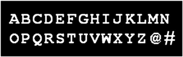
Depiction of the stimuli and mask used in the forced-choice experiments. The “M” fills a 13-wide by 12-high pixel grid.

All stimuli were displayed on 17″-diagonal PC monitors with a vertical refresh rate of 120 Hz. The display was synchronized to the vertical refresh using the ExpLib programming library Cohen and Sautner (2001). This provided a minimum display increment of 8.33 ms, but due to the occasional unintentional use of different software driver settings, the display increments for a few participants were as high as 10 ms.

The stimuli were presented in white against a black background. Each subject sat in an enclosed booth with dim lighting. The distance to the monitor (controlled by chin rests positioned approximately 60 cm from the screen) and font size were chosen such that the height of the to-be-identified letter encompassed approximately .54° of visual angle.

Responses for the 2-AFC test were collected through a standard computer keyboard. Participants were asked to press the “z”-key and the “/”-key to choose the left and right alternative respectively.

2.1.3. Procedure

Each trial began with the presentation of an “@”-sign pre-mask (300 ms) immediately followed by the target letter (for an individually adjusted duration as described below). Immediately after the offset of the target letter an “@”-sign post-mask was presented and remained until 600 ms after the first pre-mask was presented (regardless of how long the stimuli was presented). The post-mask was immediately followed by two choices presented to the right and left, with the position of the correct choice randomly determined on each trial.

The first block of 96 trials of the experiment was used to adjust the display time of the target presentation such that performance was roughly 75%. Adopting a staircase procedure, performance was evaluated every 12 trials and duration of the target presentation was adjusted at these points based on the performance in the previous 12 trials (with larger changes initially and smaller changes towards the end of the calibration period). Target letters and foils for these calibration trials were randomly chosen (with replacement) from the alphabet. After this calibration block, the display duration was not adjusted again.

Across participants, the mean presentation time obtained by using this procedure was 54 ms, but as is typical for studies using a 2-AFC perceptual identification paradigm (e.g. Huber et al., 2001 e.g. Huber et al., 2002a, b; Weidemann et al., 2005, 2008), there were large individual differences: The minimum, 25th-percentile, median, 75th-percentile, and maximum target presentation times were 10, 39, 50, 64, and 150 ms, respectively.

Following the block of 96 calibration trials, there were five blocks with 130 experimental trials each. Each block was preceded by three additional practice trials which were discarded (targets and foils for these practice trials were randomly chosen, with replacement, from the alphabet). Target and foil letters were assigned to test trials randomly with the restriction that all 650 possible combinations of targets and foils needed to be presented exactly once in the test trials of the experiment.

Feedback was given after every trial. A check-mark and the word “correct” appeared in green when the answer was correct and a cross-mark (“X”) and the word “incorrect” were presented in red when the answer was incorrect. The feedback stayed on the screen for 700 ms and was immediately followed by the presentation of the pre-mask for the next trial (unless the current trial was the last trial in a block).

After each block, participants received feedback providing the percentage of correct trials in the last block and the mean response time (this was the only time when feedback about response time was given, and the instructions emphasized accuracy rather than response speed). Between blocks, participants were encouraged to take short breaks and only resume the experiment when they were ready to continue. The entire experiment took about 45 min.

2.2. Results

Our experiment provides two measures by which letter identification performance can be assessed: accuracy and response latencies. Although accuracy is the primary dependent variable of interest, response latencies might also be of interest, even though participants were not explicitly encouraged to respond quickly. Both of these types of data are shown in Table 2, with accuracy in the top half of the table and mean response time in the bottom half of the table. For the response latencies, we eliminated the 89 trials (out of 76,700) on which the response took longer than 5 s. Otherwise, both correct and incorrect trials were included.

Table 2.

Accuracy and response time matrix for Experiment 1.

Target letter	Foil letter
	A	B	C	D	E	F	G	H	I	J	K	L	M	N	O	P	Q	R	S	T	U	V	W	X	Y	Z
A		.636	.610	.627	.729	.661	.678	.653	.814	.661	.627	.695	.695	.712	.602	.568	.568	.661	.686	.771	.619	.712	.729	.669	.644	.703
B	.814		.814	.805	.847	.839	.712	.822	.873	.856	.856	.890	.788	.864	.864	.831	.771	.814	.831	.831	.788	.847	.822	.822	.814	.873
C	.695	.729		.593	.814	.814	.661	.754	.780	.788	.729	.797	.797	.737	.508	.703	.585	.797	.720	.788	.602	.695	.763	.788	.788	.771
D	.737	.729	.686		.822	.831	.627	.780	.805	.780	.763	.788	.780	.805	.585	.797	.542	.763	.805	.890	.644	.771	.797	.847	.831	.847
E	.797	.686	.695	.695		.729	.797	.780	.890	.763	.797	.839	.746	.831	.746	.746	.729	.831	.754	.890	.703	.839	.814	.788	.763	.805
F	.814	.678	.737	.771	.593		.771	.788	.847	.814	.763	.780	.788	.720	.737	.763	.780	.695	.720	.822	.839	.831	.788	.763	.822	.771
G	.729	.686	.636	.559	.822	.831		.729	.839	.873	.763	.771	.763	.814	.669	.746	.695	.754	.771	.831	.653	.797	.771	.805	.822	.805
H	.788	.788	.788	.763	.797	.814	.746		.856	.805	.686	.831	.780	.763	.763	.729	.831	.771	.771	.780	.771	.720	.720	.754	.788	.780
I	.653	.737	.729	.729	.814	.771	.746	.754		.720	.703	.636	.771	.754	.712	.720	.746	.695	.737	.695	.746	.686	.763	.797	.695	.814
J	.746	.695	.695	.669	.703	.729	.636	.737	.712		.746	.797	.780	.788	.661	.686	.737	.712	.763	.788	.636	.788	.636	.805	.703	.703
K	.814	.822	.797	.797	.763	.746	.754	.771	.881	.839		.822	.720	.864	.788	.831	.737	.780	.763	.822	.729	.788	.805	.754	.805	.780
L	.669	.712	.746	.729	.797	.737	.805	.788	.754	.720	.695		.754	.771	.720	.746	.746	.763	.737	.695	.788	.771	.763	.780	.746	.805
M	.822	.788	.847	.847	.797	.822	.797	.771	.822	.797	.805	.864		.746	.822	.864	.831	.788	.814	.847	.797	.780	.788	.831	.831	.881
N	.780	.814	.788	.720	.856	.814	.788	.644	.873	.822	.712	.814	.780		.729	.754	.797	.712	.822	.763	.763	.754	.746	.788	.754	.797
O	.686	.729	.720	.746	.763	.839	.780	.754	.771	.805	.788	.754	.822	.771		.831	.627	.754	.788	.780	.695	.771	.746	.814	.771	.780
P	.746	.644	.686	.703	.805	.797	.695	.864	.822	.822	.814	.805	.856	.873	.729		.754	.703	.746	.822	.729	.797	.814	.814	.805	.831
Q	.695	.712	.720	.678	.788	.729	.661	.788	.797	.805	.712	.788	.746	.839	.347	.703		.720	.831	.831	.593	.754	.763	.788	.661	.763
R	.881	.771	.703	.898	.822	.839	.771	.797	.856	.763	.771	.847	.780	.873	.780	.788	.814		.754	.881	.822	.898	.771	.814	.890	.839
S	.831	.729	.780	.805	.814	.864	.746	.831	.831	.847	.805	.864	.873	.831	.805	.831	.780	.788		.814	.822	.881	.890	.873	.839	.822
T	.746	.839	.771	.780	.771	.746	.780	.805	.780	.797	.771	.797	.763	.814	.847	.822	.763	.780	.831		.847	.746	.797	.703	.797	.763
U	.771	.678	.746	.686	.814	.729	.686	.822	.788	.788	.805	.805	.788	.797	.678	.746	.619	.695	.822	.822		.712	.822	.669	.763	.805
V	.839	.856	.847	.788	.822	.873	.805	.847	.873	.839	.898	.924	.881	.907	.814	.814	.847	.839	.822	.839	.856		.814	.864	.831	.814
W	.754	.771	.754	.822	.780	.737	.805	.814	.805	.814	.754	.805	.644	.686	.805	.720	.805	.822	.754	.780	.771	.788		.780	.763	.797
X	.780	.678	.763	.678	.771	.678	.729	.754	.822	.712	.644	.797	.661	.788	.746	.771	.720	.746	.729	.805	.686	.712	.669		.686	.746
Y	.797	.839	.881	.695	.847	.771	.814	.831	.873	.856	.822	.788	.805	.771	.822	.839	.864	.873	.881	.797	.822	.695	.847	.771		.805
Z	.831	.873	.703	.788	.712	.788	.814	.754	.856	.729	.754	.729	.805	.797	.805	.712	.805	.712	.754	.814	.788	.771	.856	.746	.788
A		618	586	599	641	577	567	671	643	605	571	612	637	626	604	596	626	592	652	602	588	605	587	654	669	613
B	561		551	612	520	501	575	546	511	505	502	535	510	504	551	544	540	577	605	538	530	564	539	531	514	532
C	597	632		623	589	589	650	573	552	570	595	585	569	552	534	647	684	631	657	557	627	556	577	580	552	614
D	586	609	619		587	576	567	595	573	602	569	566	560	601	573	571	651	639	572	575	623	537	576	581	569	553
E	550	573	525	527		581	507	541	507	566	534	569	549	518	496	560	638	559	568	525	507	521	557	545	538	585
F	520	560	567	535	629		557	568	530	588	580	529	584	534	492	542	564	547	560	546	540	562	556	573	546	602
G	630	615	709	631	603	596		608	537	658	653	572	588	616	587	569	628	574	613	611	687	601	617	632	585	603
H	543	495	502	569	551	574	541		472	538	557	552	606	612	495	526	536	576	549	511	574	594	585	528	526	546
I	516	495	512	558	545	577	522	521		553	570	578	521	518	483	518	456	494	477	583	563	526	546	518	578	530
J	525	582	559	538	586	553	560	597	607		591	598	569	568	530	538	572	584	571	604	543	538	583	610	599	585
K	515	503	541	548	572	538	504	560	468	528		532	622	585	557	491	543	524	537	528	547	487	588	569	532	599
L	546	517	512	518	532	611	489	530	562	591	535		535	491	500	530	560	576	507	556	508	510	592	514	560	529
M	498	515	497	506	493	604	483	617	500	483	504	524		567	506	497	496	524	581	514	528	534	603	517	506	465
N	536	506	523	554	579	520	557	586	483	534	576	551	585		537	500	506	535	493	491	497	572	615	596	559	549
O	586	677	646	622	597	572	555	602	621	622	643	598	640	600		595	598	598	574	530	667	611	565	599	593	609
P	507	552	555	567	546	553	541	556	504	512	544	521	517	556	531		548	572	612	548	511	471	564	528	507	552
Q	647	603	670	619	628	572	784	640	587	566	642	597	641	624	672	637		599	609	661	697	662	654	632	641	621
R	550	564	574	543	555	535	533	546	500	507	556	511	574	523	542	558	539		552	575	512	531	567	489	493	570
S	533	591	546	519	600	547	506	486	507	505	518	498	529	518	584	557	530	554		555	479	490	552	537	504	538
T	491	462	452	458	567	509	491	526	540	559	499	540	491	526	518	487	530	534	476		487	560	570	567	523	558
U	541	624	582	685	544	545	620	549	604	635	561	595	592	552	525	612	633	655	581	523		610	551	573	572	608
V	457	478	464	494	495	515	480	544	494	476	520	537	525	531	501	462	535	483	505	506	558		501	495	536	510
W	554	525	515	507	542	556	543	575	499	511	609	593	635	631	493	533	504	495	572	548	542	560		593	551	545
X	615	556	519	533	574	575	516	551	587	541	570	542	567	614	494	533	531	557	596	587	581	634	617		589	581
Y	534	494	467	491	571	488	456	586	531	497	508	570	451	495	496	494	509	493	484	556	516	579	583	544		518
Z	567	542	566	562	563	566	553	609	580	602	611	590	576	607	493	547	532	573	490	571	568	545	527	518	570

Note. Values in top half of table indicates the proportion of participants who responded correctly for each target-foil combination. Values in the bottom half indicate the mean response time (in ms) for correct and incorrect responses.

Correct responses were made on average 110 ms faster than incorrect responses (542 ms vs. 652 ms), which was highly reliable (t(117)=9.05, p<.01). Across the 650 cells in Table 2, this manifested as a Pearson's correlation of −.49, which was statistically reliably negative (p<.001). This correlation is not unexpected, but because of this relationship between speed and accuracy, and because the task was designed to measure response accuracy, we performed all subsequent analyses using only the accuracy values found in Table 2.

The data shown in Table 2 are perhaps too complex to easily make sense of. We have therefore plotted mean accuracies from Table 2 in Fig. 2, with respect to the target (top panel) and foil (bottom panel).

Fig. 2.

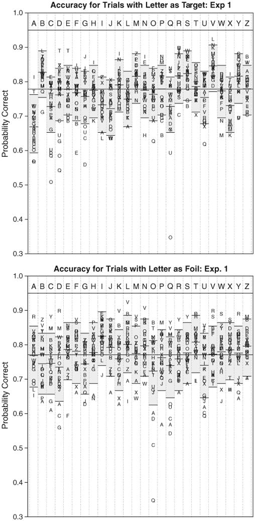
Accuracy for letter combinations in Experiment 1, for letter pairs sorted by target (top panel) or by foil (bottom panel). The gray boxes in each column depicts the 96% confidence range for each target-foil combination, using a bootstrapping process to incorporate between-participant variability in mean accuracy. Observations well outside these bounds correspond to conditions where (top) bias and similarity are strong, or (bottom) perceivability and similarity are strong. Exact values are listed in Table 2.

For each target letter, the mean accuracies across the 25 foils would be expected to have a binomial distribution, if there were no impact of bias or similarity and if all participants were identical. For a binomial distribution with mean .77 and 118 observations (as in our experiment), the standard error of the estimate is $\sqrt{\frac{.75\times 25}{118}}=.0387$. Our data violate this binomial model, such that 103 out of 118 participants had mean accuracies that fell outside the 95% confidence range of .743 to .798. Consequently, we simulated ranges for each letter via a bootstrapping technique, as follows. First, a single log-odds factor was estimated for each participant that determined how much better or worse his or her mean accuracy was (across the entire experiment) than average. These deviations were then used to create a hypothesized distribution of binomial parameters for each target character, and a 95% confidence interval was created empirically by first sampling a participant, adjusting the accuracy in log-odds space by the factor assumed for each participant, and using this adjusted factor to run a binomial trial and determine whether the comparison was correct or incorrect. For each column, 5000 experiments of a size equal to Experiment 1 were simulated in this fashion, and the gray rectangle represents the 95% confidence region around the mean accuracy for that target.

Fig. 2 illustrates a number of qualitative phenomena that suggest each of the three factors of perceivability, bias, and similarity are at play in our experiment. For example, a hallmark of high or low perceivability is that a target's accuracy should rise or fall regardless of the foil, (not just because of a few foils). This type of effect occurred for a number of target letters (for example, “A”, “J”, “Q”, and “X” tend to show below-average accuracy, and “B”, “M”, “R”, “S”, and “V” exhibit above-average accuracy across most foils). These effects are not isolated to just the mean accuracy, but impact the target accuracy for almost all foils. Furthermore, a hallmark of high or low bias is that a foil's accuracy should rise or fall regardless of the target. Although bias will impact a target as well, perceivability should not depend on the foil, and so bias effects should typically impact accuracy regardless of the target (for example, this is seen for the foils “I”, “L”, and “Z”, which tend to produce higher than average accuracy, and the foils “D”, “O”, “U”, which are associated with lower than average accuracy across many targets). Finally, a signature of a similarity effect is that a letter pair deviates from the impact that would be seen from the bias and perceivability alone. A number of individual letter pairs match this pattern (such as combinations of “O”, “Q”, and “D”).

This qualitative analysis also suggests several phenomena related to the post-stimulus mask. First, the target that was least accurate was the “A”. This may have occurred because the “@” mask, which contains a lowercase “a”, somehow interfered with correct identification of the “A”. Another provocative result revealed by Fig. 2 is that when a round letter (i.e., “O”, “D”, “Q”, “U”, “G”, or “C”) appeared as a foil, accuracy suffered. These letters are visually similar to the “@” mask, and this similarity may lead people to choose the foil more often when it was round, resembling the mask. Finally, accuracy for these round letters was not especially improved when they appeared as targets, indicating that the visually similar mask interfered with perceptual identification, despite participants' increased tendency to choose them. Several foil letters led to above-average accuracy (i.e., “I”, “T”, and “L”). These letters stand out as being very dissimilar to both the mask and to other letters, indicating that people may have been more easily able to eliminate this option and select the target correctly.

These initial results of Experiment 1 indicate that the shape and identity of the mask may affect letter identification accuracy in important ways. To better investigate this influence, we carried out a second (otherwise identical) experiment using a different commonly-used mask.

3. Experiment 2

3.1. Method

3.1.1. Participants

Ninety-six undergraduate students at Indiana University participated in exchange for introductory psychology course credit.

3.2. Materials, equipment, and display, and procedure

The procedure used in Experiment 2 was identical to Experiment 1 in every way, except for the use of the “#” symbol instead of the “@” symbol as a post-stimulus mask. The mask was adjusted in font and size (“Arial Bold”, 17 pt.) to cover the display area of the letters. A depiction of this mask is shown in Fig. 1.

3.3. Results

As with Experiment 1, letter identification performance can be assessed by examining both the accuracy and response latencies of trials in which one stimulus was a target and the other was the foil. These data are shown in Table 3, with accuracy in the top half and mean response time in the bottom half of the table. For the response latencies, we eliminated the 262 trials (out of 62,400) on which the responses took longer than 5 s. Otherwise, both correct and incorrect trials were included.

Table 3.

Accuracy and response time matrix for Experiment 2.

Target Letter	Foil Letter
	A	B	C	D	E	F	G	H	I	J	K	L	M	N	O	P	Q	R	S	T	U	V	W	X	Y	Z
A		.810	.845	.724	.741	.759	.707	.724	.879	.845	.707	.828	.759	.810	.793	.828	.914	.741	.793	.862	.862	.707	.707	.810	.741	.810
B	.724		.776	.638	.724	.724	.672	.690	.862	.776	.828	.828	.793	.776	.672	.672	.672	.724	.879	.793	.759	.741	.862	.690	.810	.759
C	.845	.845		.759	.845	.862	.672	.845	.828	.793	.845	.776	.862	.879	.741	.828	.759	.862	.845	.845	.724	.862	.862	.897	.759	.862
D	.862	.862	.862		.810	.776	.845	.828	.828	.914	.897	.897	.828	.862	.828	.810	.793	.879	.828	.828	.759	.810	.845	.793	.879	.897
E	.810	.638	.776	.707		.603	.759	.638	.862	.759	.690	.621	.724	.690	.759	.603	.810	.655	.638	.810	.741	.810	.741	.741	.810	.707
F	.707	.759	.793	.759	.603		.741	.776	.776	.810	.793	.862	.741	.879	.724	.724	.776	.707	.793	.621	.759	.724	.741	.741	.776	.655
G	.793	.724	.603	.759	.793	.828		.845	.845	.828	.707	.810	.810	.828	.776	.776	.690	.741	.879	.845	.793	.828	.776	.897	.776	.845
H	.552	.724	.707	.621	.638	.569	.741		.655	.603	.655	.724	.586	.586	.690	.517	.741	.534	.776	.690	.638	.655	.603	.655	.603	.569
I	.517	.431	.448	.586	.448	.414	.655	.569		.448	.431	.414	.466	.552	.638	.500	.586	.466	.466	.534	.638	.379	.466	.466	.466	.414
J	.741	.569	.690	.638	.776	.672	.690	.759	.879		.759	.724	.638	.724	.672	.690	.586	.724	.707	.759	.672	.690	.638	.707	.707	.707
K	.655	.759	.810	.793	.672	.776	.741	.741	.810	.828		.793	.690	.759	.810	.776	.776	.621	.776	.724	.828	.759	.621	.707	.828	.707
L	.707	.655	.638	.724	.672	.603	.810	.655	.741	.655	.655		.552	.707	.655	.707	.793	.603	.690	.621	.603	.586	.621	.586	.655	.707
M	.776	.724	.793	.845	.828	.741	.793	.707	.897	.862	.707	.828		.724	.862	.810	.741	.707	.828	.931	.845	.759	.621	.741	.845	.690
N	.793	.724	.862	.690	.690	.759	.845	.707	.776	.810	.759	.690	.672		.741	.810	.759	.707	.759	.810	.776	.655	.741	.690	.724	.776
O	.776	.879	.845	.810	.879	.828	.897	.776	.914	.828	.810	.879	.948	.862		.793	.741	.793	.931	.897	.862	.897	.810	.828	.810	.845
P	.793	.672	.793	.672	.810	.793	.845	.672	.759	.690	.759	.862	.793	.776	.862		.776	.793	.828	.828	.741	.776	.672	.707	.828	.793
Q	.828	.707	.724	.621	.828	.759	.810	.828	.776	.793	.793	.862	.879	.793	.483	.828		.776	.741	.810	.690	.845	.845	.724	.828	.793
R	.810	.793	.724	.759	.776	.879	.759	.810	.828	.793	.793	.828	.724	.793	.810	.793	.879		.724	.828	.810	.741	.793	.759	.776	.810
S	.793	.638	.724	.707	.741	.690	.724	.810	.759	.741	.879	.759	.793	.776	.776	.724	.741	.672		.759	.793	.741	.845	.845	.793	.828
T	.638	.638	.741	.638	.672	.483	.690	.621	.741	.638	.552	.741	.638	.638	.638	.655	.672	.621	.672		.621	.707	.707	.552	.707	.638
U	.828	.776	.793	.707	.741	.828	.707	.776	.810	.828	.759	.759	.793	.741	.672	.776	.672	.776	.828	.862		.793	.759	.828	.810	.828
V	.586	.845	.810	.724	.845	.776	.828	.845	.828	.793	.776	.810	.759	.741	.759	.724	.690	.810	.793	.810	.828		.741	.776	.828	.845
W	.759	.828	.724	.690	.586	.690	.655	.603	.776	.810	.759	.741	.638	.707	.845	.776	.828	.690	.810	.793	.655	.741		.724	.690	.690
X	.638	.603	.655	.655	.586	.569	.741	.621	.707	.655	.466	.690	.603	.621	.724	.621	.655	.707	.707	.655	.776	.621	.621		.552	.690
Y	.672	.552	.638	.776	.690	.655	.672	.638	.776	.810	.586	.569	.603	.741	.707	.672	.672	.621	.707	.741	.655	.586	.603	.655		.655
Z	.672	.741	.793	.810	.759	.759	.810	.793	.776	.690	.690	.845	.845	.845	.810	.793	.810	.793	.655	.776	.724	.655	.707	.586	.897
A		509	570	644	510	581	550	590	558	528	572	582	528	522	511	474	594	594	571	508	531	573	547	561	524	533
B	597		547	594	607	553	638	582	559	586	623	569	526	562	578	569	618	597	551	536	633	519	614	584	591	585
C	508	539		521	521	560	646	518	521	487	490	493	528	509	587	557	590	469	527	505	579	524	529	538	566	568
D	524	553	540		532	521	556	474	499	555	499	499	535	524	589	520	597	505	517	550	564	560	492	495	504	545
E	610	617	613	557		590	617	580	618	555	552	594	596	525	606	575	560	631	632	631	645	506	595	604	567	716
F	596	584	541	565	634		527	585	613	665	632	564	585	598	532	602	522	585	588	577	542	604	625	608	584	590
G	544	581	755	583	555	570		546	541	517	534	509	517	521	576	551	693	534	539	567	589	604	518	584	541	562
H	655	651	694	692	707	714	623		584	602	685	644	726	711	638	653	647	710	610	673	679	638	658	715	593	619
I	664	621	571	624	730	721	678	690		625	589	711	724	633	626	629	630	698	660	630	672	647	660	721	647	688
J	586	586	534	666	601	578	623	668	560		638	565	617	561	529	598	626	662	581	620	576	594	637	604	607	582
K	628	531	516	604	672	587	557	615	572	584		599	537	608	523	555	607	572	564	593	649	637	674	634	593	630
L	573	576	516	589	589	582	626	519	622	615	570		552	542	592	545	533	563	571	581	531	553	558	657	609	608
M	635	601	571	627	645	585	582	729	586	527	568	567		611	552	589	560	627	541	577	567	596	778	621	614	617
N	594	557	542	561	611	644	546	669	540	571	610	536	713		632	615	563	593	611	622	549	660	680	663	589	599
O	457	506	547	477	479	466	483	447	464	476	488	511	506	506		504	605	492	495	449	505	472	479	497	554	534
P	536	596	619	487	571	543	551	548	484	532	592	503	564	564	508		525	605	577	499	537	474	480	555	484	501
Q	558	576	612	688	567	569	682	556	587	504	552	545	510	562	654	599		577	559	616	601	558	616	598	604	620
R	571	547	515	533	596	509	540	547	523	624	551	528	551	548	512	581	583		572	506	515	573	561	501	536	545
S	598	612	579	546	535	540	570	544	559	640	559	571	564	559	523	608	642	631		619	571	550	584	637	567	615
T	607	609	557	621	617	603	573	656	650	612	680	642	626	600	606	650	581	596	635		633	655	634	646	671	578
U	619	572	552	583	537	587	623	540	606	573	508	570	523	581	611	541	627	615	629	543		552	560	570	548	560
V	595	540	525	569	544	551	548	553	595	617	587	546	574	596	601	510	575	576	547	591	614		603	591	614	573
W	593	674	582	618	554	606	538	675	627	611	717	614	688	620	589	601	589	595	591	688	617	723		629	662	617
X	616	709	649	628	667	655	630	647	644	774	670	634	725	728	575	692	633	611	660	671	573	672	623		749	691
Y	639	621	615	624	687	613	592	727	661	698	607	736	670	599	576	598	577	573	588	641	637	671	651	662		718
Z	582	510	563	552	582	575	526	548	474	560	557	549	558	522	570	565	565	595	524	587	581	620	538	601	594

Note. Values in top half of table indicates the proportion of participants (out of 96) who responded correctly for each target-foil combination. Values in the bottom half indicate the mean response times for correct and incorrect responses.

In Experiment 2, correct responses were made on average 93 ms faster than incorrect responses (581 ms vs. 674 ms), which was highly reliable (t(95)=7.4, p<.01). Across the 650 cells in Table 3, this manifested as a Pearson's correlation of −.38, which was reliably negative (p<.001). As with Experiment1, we performed all subsequent analyses on the accuracy data only.

Fig. 3 depicts the accuracies for each letter combination, sorted by target and foil. As we found in Experiment 1 (cf. Fig. 2), there were consistent deviations in accuracy when letters appeared as targets, and also when letters appeared as foils. The 96% confidence range for each target is shown as a shaded region in each column, and the confidence range for the means are also shown by the horizontal lines. Again, as with Experiment 1, these confidence ranges are simulated via a bootstrapping procedure that incorporates between-subject variability in mean performance (the expected binomial 95% range for participant means was .726 to .781, and 82/96 participants fell outside that range).

Fig. 3.

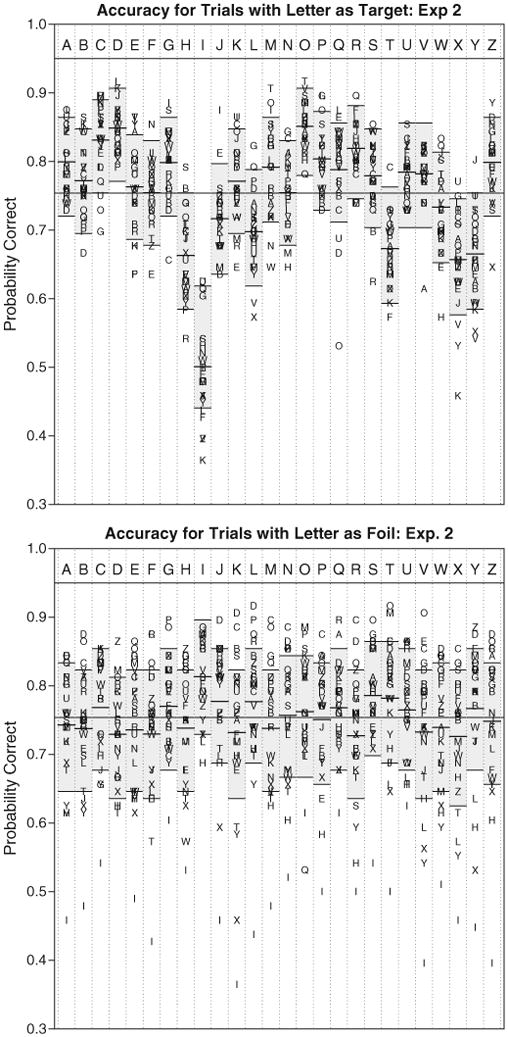
Accuracy for letter combinations in Experiment 2. Top panel shows accuracy for letter pairs sorted by target (top panel) or by foil (bottom panel). The gray boxes in each column depicts the 96% confidence range for each target-foil combination, using a bootstrapping process to incorporate between-participant variability in mean accuracy. Observations well outside these bounds correspond to conditions where (top) bias and similarity are strong, or (bottom) perceivability and similarity are strong. Exact values are listed in Table 3.

One surprising result, shown in Fig. 3, is that participants were extremely poor at identifying the target letters “I” and “T”. Accuracy was above average on trials when either was presented as a foil, indicating a bias against making these responses. Overall, many letters containing vertical and horizontal features (“I”, “T”, “H”, perhaps including “X”) were identified less accurately when they were targets, whereas letters with round shapes (“O”, “D”, “C”, “G”, “R”) did not produce below-average accuracy as in Experiment 1. Unlike Experiment 1, the letter “A” was identified with above average accuracy.

These qualitative descriptions of the data are difficult to evaluate on their own, because in many cases the identification accuracy appears to depend on the letter presented, the foil, and the mask. Next, we will present a model that attempts to quantitatively estimate the simultaneous contributions of perceivability, similarity, and bias to these patterns of results.

4. Modeling the sources of letter detection accuracy

Our review of the literature suggests that conceptually, letter detection accuracy may be influenced by perceivability, bias, and similarity. Yet few (if any) quantitative attempts have been made to estimate these three factors simultaneously for the alphabet. Most previous attempts have decomposed accuracy into two fundamental factors, typically using a version of the “similarity” or “biased” choice model (Luce, 1963; Shepard, 1957). This theory constitutes an axiomatic model of how biases, similarities, and the number of choice alternatives impact detection accuracy. Other alternatives have been discussed previously, (cf. Smith, 1992; Townsend, 1971a), which typically involve different mathematical forms for combining influences of similarity and bias. We will adopt a fairly theory-agnostic statistical model of the joint impacts of perceivability, response bias, and similarity which (as we show in the Appendix) permits interpretation in terms of the biased choice model.

4.1. A statistical model of letter detection

We developed the statistical model presented here specifically to illustrate how the data from our two experiments can be used to simultaneously estimate perceivability, bias, and similarity. For our 2-AFC procedure, each cell of the confusion matrix is assumed to be measured independently. Each of the N(N − 1) = 650 cells produced an accuracy value, which we will represent as p_i,j, where i represents the target letter and j represents the foil. No observations are made for cell i = j, which differs from naming studies, in which the diagonal i = j indicates correct responses, and typically represents the bulk of the data. Thus, there are at most N(N − 1) degrees of freedom for each experiment. The model attempts to estimate log-odds accuracy $\left(ln\left(\frac{p_{i,j}}{1-p_{i,j}}\right)\right)$ based on a linear combination of other factors.

In our model, we assume that a percept is produced that may differ somewhat from the target stimulus, and this difference affects the accuracy for the target in general, regardless of the foil. We estimate the extent to which this difference affects accuracy with paramet.er λ_i, which describes the perceivability of stimulus s_i in log-odds units. If the value of λ_i were 0, (with no other contributors), this would produce a log-odds accuracy value of 0 (or 50% accuracy) for that stimulus. As λ_i increases, baseline accuracy for that stimulus increases. For convenience, we estimate a baseline intercept (μ) which represents the overall perceivability within an experiment, and estimate individual values of λ relative to this intercept. Consequently, positive values indicate greater than average perceivability, and negative values indicate smaller than average perceivability, and a full estimate of perceivability for a letter i can be computed as μ+ λ_i. In the baseline model where a perceivability parameter is estimated for each letter, Σ_iλ_i = 0, which is logically necessary to allow the intercept to be estimated.

Several psychological processes could influence λ_i. For example, perceivability may have its impact during early perceptual stages, affecting the probability that an accurate image is perceived, perhaps distorted through internal or external noise sources. Our model does not distinguish between these sources, although one could if proper experimental procedures were employed (cf. Mueller and Weidemann, 2008). Alternately, λ_i may be influenced by some aspect of the comparison process, assessing the similarity between a percept and the displayed response option. If a mask consistently introduced or erased features from the percept of a particular character, this would likely result in a lower value for λ_i; if it consistently erased features across all stimulus characters, the baseline intercept might be reduced instead.

Next, we assume that response biases exist for each of the two response alternatives. We denote bias with the symbol γ_i for response alternative i, and assume that it also impacts log-odds accuracy linearly. If γ_i is 0, the observer has no bias for a specific alternative. Positive values of γ_i indicate bias toward a response, so a positive bias for a target and/or a negative bias for a foil improves accuracy. In the baseline model where a bias parameter is estimated for each letter, the bias values are also constrained to sum to 0.

Finally, we assume that the similarity between the percept of the stimulus and that of the foil impacts log-odds response accuracy linearly. In the model, we define a parameter corresponding to the dissimilarity between stimulus i and response j on log-odds accuracy called δ_i,j. For δ, a value near 0 indicates that the accuracy can be well explained by the estimated perceivability and bias main effects alone. Positive δ values indicate greater dissimilarity, such that the letter pair is particularly easy to distinguish. Conversely, negative δ values indicate greater confusability, and produce lower accuracy than would be expected from bias and perceivability alone. Note that there might also be a number of distinct psychological interpretation of δ_i,j. Many approaches are often interested in the (dis)similarity between canonical representations of letter forms, but for our experiment (in which the foil response is not known before the stimulus flash), δ really estimates the dissimilarity between a noisy target percept and the percept of the response alternative following stimulus presentation. Under this interpretation, perceivability is really just another type of dissimilarity: the distinctiveness between the noisy target percept and the correct response option (as opposed to the incorrect response option). As we show in the Appendix, perceivability thus corresponds to δ_i,i.

A simple model might attempt to account for log-odds accuracy based on an intercept μ, N perceivability parameters λ (with at most N − 1 degrees of freedom), N bias parameters (again with at most N − 1 degrees of freedom), and N² − N similarity parameters. Obviously, there are more predictors than data in such a model, so we will always constrain similarity to be a symmetric (δ_i,j = δ_j,i), which contributes only N*(N − 1)/2 parameters to the predictive model. This model, too, is non-identifiable, and so one can also introduce other constraints, such as Σ_i,jδ_i,j = 0 or Σ_iλ_i = 0. However, we avoid making these assumptions by adopting a parameter selection method that uses only parameters that are relatively powerful at accounting for data. Parameter selection has been used frequently in linear regression models to help identify parsimonious and descriptive models with relatively few parameters (e.g. Hoeting et al., 1996; Mitchell and Beauchamp, 1988; O'Gorman, 2008; Yamashita et al., 2007). These methods are especially useful in cases such as ours, where the number of possible predictors is in fact greater than the degrees of freedom in the data. Using this method, we retain the constraint that δ_i,j = δ_j,i, but no other row or column sum constraints are needed–when a parameter is removed from the model, it frees up a degree of freedom to be used to estimate the intercept or higher-order main effects.

One theoretical benefit of using a parameter selection method (in contrast to traditional factorial approaches) is clear if one considers two target characters in a hypothetical experiment with five foil characters. Suppose the targets each have a mean accuracy of 0.75; one because its accuracy is .75 for each foil it was compared to, and the second because for four of the foils, its accuracy is .8125, but for the remaining foil, its accuracy is 0.5 (0.8×0.8125 + 0.2×0.5 = 0.75). A complete factorial model would estimate a mean accuracy of .75 for each target, estimating five similarity scores of 0 for the first target, and four slightly positive and one large negative similarity score for the second target. But if one allows non-critical parameters to be removed from the model, the first target's mean accuracy would again be .75, with the five similarity parameters removed from the model. In contrast, the second target's mean accuracy would rise to .8125, with a single additional similarity parameter to account for the below-average foil. Thus, variable selection can provide a relatively parsimonious coding that matches an intuitive explanation of data: we argue it is simpler and more intuitive to describe the accuracy for the second target as .8125 (with one exception), instead of saying it is .75, and then describing the deviation for each individual foil.

Overall, the model falls into a family described by Eq. (1):

$$ln\left(\frac{p_{i,j}}{1-p_{i,j}}\right)\propto \mu +{\lambda }_i+{\gamma }_i-{\gamma }_j+{\delta }_{i,j}$$ (1)

To apply the model to both experiments, we extend Eq. (1) as follows:

$$ln\left(\frac{p_{i,j}^{\left[x\right]}}{1-p_{i,j}^{\left[x\right]}}\right)\propto \mu +{\lambda }_i^{\left[x\right]}+{\gamma }_i^{\left[x\right]}+{\gamma }_j^{\left[x\right]}+{\delta }_{i,j}+{\delta }_{i,j}^{\left[x\right]}+{\delta }_{i,j}^{\left[2-1\right]}$$ (2)

where the δ_i,j parameter allows an overall pairwise similarity estimate to be made, and the ${\lambda }_i^{\left[x\right]}$, ${\gamma }_j^{\left[x\right]}$, and ${\delta }_{i,j}^{\left[x\right]}$ parameters allow an experiment-specific value to be estimated. The parameter ${\delta }_{i,j}^{\left[2-1\right]}$ is used to indicate a contrast coding between experiments, enabling a differential similarity parameter to be estimated. When present, the value is added to the relevant pairs in Experiment 1 and subtracted from the same pairs in Experiment 2.

Model parameters were estimated by fitting a linear regression to account for log-odds accuracy with the appropriate combination of intercept, perceivability, bias, and dissimilarity parameters, as specified in Eq. (2). To identify a minimal set of parameters that reliably accounted for the data, we used a stepwise regression procedure available in the stepAIC function of the MASS package (Venables & Ripley, 2002) of the R statistical computing environment (R Development Core Team, 2008), using the Bayesian Information Criterion (BIC; Schwarz, 1978) to determine which parameters should be included in the model. Bayesian model selection schemes have been increasingly used to select between models in psychology, and especially between models of perception such as choice theory (cf. Myung, 2000; Myung & Pitt, 1997; Pitt et al., 2002, 2003). The BIC statistic combines maximum likelihood goodness of fit with a penalty factor for model complexity (k log ₂(N) for k parameters and N data points), so that a parameter is only retained in the model if its goodness of fit improves more than the complexity penalty term. In general, Bayesian model selection methods attempt to counteract the tendency to create over-parameterized models that fit the data but are unable to generalize. In our case, it also helps us to select a parsimonious model from among a family of inconsistent possibilities, to allow the most appropriate model for the data to be selected.

This approach begins with an appropriate minimal model (e.g., the intercept only model), and then fits all models with one additional parameter that are subsets of the complete model, on each step choosing the model that has the smallest BIC score. This procedure continues, on each following iteration fitting all models that differ from the current model by one parameter (either by including a new parameter or excluding parameter that had previously been used). This stepwise procedure is generally more robust than pure parameter-adding or parameter-trimming selection methods that only search in one direction, at the cost of slower search.

We also fit a number of benchmark and sub-models to serve as comparisons. The outcomes of several of the most interesting models are shown in Table 4. Two models form the extremes of the model selection search: at one end, the fully-specified Model 1 incorporating similarity, bias, and perceivability parameters for both experiments (with proper constraints); and at the other end, the intercept-only Model 8.

Table 4.

Summary of models predicting log-odds accuracy based on various predictor sets.

	Model name	BIC	R2	Adjusted R2	RSE	F Statistic
1.	Full model	4162	.9823	.9616	.253	F(699,600) = 47.5
2.	Intercept + BIC-selected bias, similarity, and general perceivability	592	.666	.648	.259	F(66,1234) = 37.8
3.*	Intercept + BIC-selected bias, similarity, general & specific perceivability	572	.692	.672	.2498	F(77,1222) = 35.7
4.	Full bias + similarity (Biased choice rule)	4162	.845	.665	.253	F(699,600) = 4.68
5.	Bias + Similarity (BIC-Selected)	1000	.65	.617	.269	F(114,1185) = 19.43
6.	Bias + Perceivability (BIC-selected)	734	.577	.562	.289	F(42,1257) = 40.8
7.	Similarity + Perceivability (BIC-selected)	715	.597	.581	.283	F(48,1251) = 40.8
8.	Intercept-only model	1549	n/a	n/a	.4367	t(1299) = 100

Note: RSE = residual standard error (error sum of squares divided by the residual degrees of freedom). General similarity refers to a single set of similarity parameters fit across experiments. Specific similarity refers to using similarity parameters that can account for each experiment individually. Model 3, indicated with a *, indicates our preferred best model.

The variable selection method serves to search through sub-models of this baseline Model 1, including only parameters that increase the predictability considerably. The only parameter required in all models was the intercept parameter, and we used a single common intercept across experiments, which produced reasonable model fits. Because accuracy was around 75%, which corresponds to an odds ratio of 3:1, we expect the fitted μ parameters to have a value around ln(3/1) = 1.1 (the actual fitted value of or final Model 3 was 1.3).

In all of the models, we allowed each experiment to have individual perceivability and bias parameters, because other versions which constrained perceivability and bias parameters to be identical across experiments produced unsatisfactory model fits. We next fit a Model 2, in which we used a single set of similarity values across both experiments. This model performed relatively well, with a relatively low BIC statistic. We compared this to Model 3, in which we selected from the full set of similarity parameters in Eq. (2). In this model, for any letter pair, four different candidate similarity parameters were available: one for each experiment, one for both experiments, and one for the difference between Experiment 1 and Experiment 2. These parameters are redundant and so only two of the four could ever be selected for a given letter pair. The resulting Model 3 provided the best overall BIC score, and we will examine the obtained parameter values in greater detail below.

The fitted parameter values for Model 3 are found in Table 4. Only parameters that were reliably different from 0 were chosen, so blank entries can be interpreted as having a default value of 0. The right columns of the table show similarity effects: either global parameters that applied to both experiments, experiment-specific parameters that indicate how the mask impacts dissimilarity, and “differential dissimilarity”: situations where in one experiment the pair was less similar than the default, and in the other experiment the pair was more similar than default.

After selecting parameters using the BIC criterion, 20/52 perceivability parameters and 16/52 bias parameters remained. Experiment 2 required more of both bias and perceivability parameters. The sign of the perceivability parameters seems somewhat related to the shape of the mask: In Experiment 1, negative parameters were estimated for A, C, J, and X, and for Experiment 2, for F, H, I, J, L, T, W, X, and Y. There was essentially no relationship between these two sets of parameters, indicating that the mask has idiosyncratic impacts on the perceivability of individual letters. In general, negative parameters were found for letters with global shape similarity to the mask, and positive parameters tended to have global shape dissimilarity. However, it is not true that letters with strong similarity to the mask had universally poor perceivability. For example, most of the round letters in Experiment 1 did not have a low perceivability value (D, G, O, Q, U)–their poor performance can mostly be attributed to confusions amongst them, rather than an overall decrease in perceivability.

A few additional models were fit for comparison, which help illustrate the relative contributions of the different parameters. Model 4 represents the biased choice model, allowing only bias and similarity parameters. Its BIC score is much higher, but it is somewhat unfair to compare that model to our preferred Model 3, in which full parameter selection techniques were allowed. Consequently, we fit Model 5, which was a biased choice model that used parameter selection in an identical way to Model 3 (selecting among four similarity parameters per letter pair, and selecting only the bias parameters that were deemed reliable). This model produce BIC scores that were much worse, and used slightly more bias parameters (24 versus 16) and substantial more similarity parameters (115 versus 78) in comparison to Model 3. These additional similarity parameters included large sets that seem to account for similarity between a single letter and many other letters. For example, consider “H” and “I”, whose accuracies were overall fairly low in Experiment 2. Model 5 estimated negative bias for these letters, but nine similarity parameters for H and 13 parameters for I. So, to account for the lower accuracy, the biased choice model must assume that H and I become more similar to nearly half the letters of the alphabet. In contrast, by using two perceivability parameters related to H and I, Model 3 reduces the similarity parameters to just four: one differential similarity value involving I, and one similarity value for H specific to Experiment 2. In other words, although the overall decrease in accuracy for H and I in Experiment 2 could logically be attributed to a change in the similarity space, a simpler account is that their perceivability was reduced: an account much more in line with the hypothesized impact of the visually-similar # mask. This illustrates how perceivability parameters are important for accounting for the data, and thus should be taken seriously as a theoretical construct.

Finally, Models 6 and 7 couple perceivability with either bias or similarity (but not both). Model 6 used the stepwise BIC procedure to select bias and perceivability parameters. This model is substantially worse than those that also incorporated similarity parameters (e.g., Models 2 and 3), while selecting roughly the same number of bias and perceivability parameters (16 and 24, respectively) as Model 3 (which selected 16 bias and 20 perceivability parameters). This indicates that the remaining similarity parameters are critical for accounting for the data. Interestingly, Model 6 performs better than the bias + similarity models (Models 4 and 5), even though it could not use any of the 325 similarity parameters, showing the power of perceivability parameters. In contrast, Model 7 uses the stepwise BIC-selected parameters to select perceivability and similarity parameters (with no bias). Here, we used one set of similarity parameter per experiment(rather than the full complement of four), but the results are similar. The model selected 23 perceivability parameters (compared to 20 in Model 3), and 25 similarity parameters (compared to 17 global similarity parameters+26 experiment-specific values in Model 3). The model is slightly better than the biased choice model, but still much worse than Model 3. Together, these models illustrate the incremental validity of each factor, and demonstrate how together, they provide the most parsimonious account of the data.

The fitted parameters in Table 5 can be used to compute predicted accuracies for any condition in the experiments. For example, to determine the predicted accuracy for “A” with the “B” foil in Experiment 1, one adds together the intercept (1.306), the perceivability for “A” (−0.57), the bias for “A” (0.0), the dissimilarity between “A” and “B” (0), and subtracts the bias for “B” (.227). This estimates the log-odds accuracy for that condition to be 1.306−.57−.227=0.509, which corresponds to a probability of .624 (the actual accuracy for this condition was .636). Fig. 4 shows the predicted accuracies for Experiments 1 and 2, based on the parameters in Table 5. It should be evident that the parameter selection techniques tend to place most points at the intercept, because there is little evidence to suggest they differ from the default accuracy. Variability in the mean accuracy across targets (columns) stems from differences in the perceivability parameters; variability within a column tends to stem from bias parameters (when a foil is high or low relative to most targets), or from individual pairwise similarity values.

Table 5.

Reliable parameters from Model 3 using the BIC model selection technique. Smaller and more negative values indicate that a letter was less perceivable, biased against, or that a letter combination was discriminated less well than was expected by the perceivability and bias alone. Baseline log-odds accuracy was 1.306 which is equivalent to a percent accuracy of 78.7, which was restricted to be the same across both experiments.

Letter	Experiment 1 (“@”)		Experiment 2 (“#”)		Global Dissimilarity (δ)			Experiment-specific Dissimilarity (δ)
	Perceivability (λ)	Bias (γ)	Perceivability (λ)	Bias (γ)
Intercept	1.306		1.306
A	−0.571				B	G	−0.388	Experiment 1
B		0.227			C	G	−0.737	B	Z	0.621
C	−0.174		0.602	−0.206	C	O	−0.686	C	D	−0.638
D			0.208	0.155	C	Q	−0.540	D	G	−0.927
E					C	U	−0.364	D	O	−0.597
F			−0.153		D	Z	0.349	D	Q	−0.849
G				−0.230	E	F	−0.648	D	U	−0.618
H			−0.612		H	N	−0.457	E	I	0.475
I		−0.273	−0.948	−0.346	I	L	−0.335	G	Q	−0.560
J	−0.338		−0.242	−0.146	K	M	−0.345	G	U	−0.599
K					K	X	−0.355	O	U	−0.522
L		−0.164	−0.573	−0.191	M	N	−0.424	R	Y	−0.600
M	0.246				M	W	−0.468
N				−0.118	N	W	−0.408	Experiment 2
O			0.672	−0.161	O	Q	−1.152	A	V	−0.551
P					Q	U	−0.646	D	L	0.653
Q					X	Y	−0.342	E	K	−0.635
R		0.171		0.148				F	T	−0.497
S	0.258			−0.126				G	L	0.482
T			−0.382	−0.199				G	X	0.473
U					Differential Dissimilarity			H	W	−0.494
V	0.422				A	Q	−0.472	L	P	0.663
W			−0.251		E	N	0.360	L	Q	0.621
X	−0.25		−0.851	0.161	G	P	−0.413	Q	R	0.470
Y	0.204		−0.626		I	Z	0.379
Z					U	X	−0.415

Fig. 4.

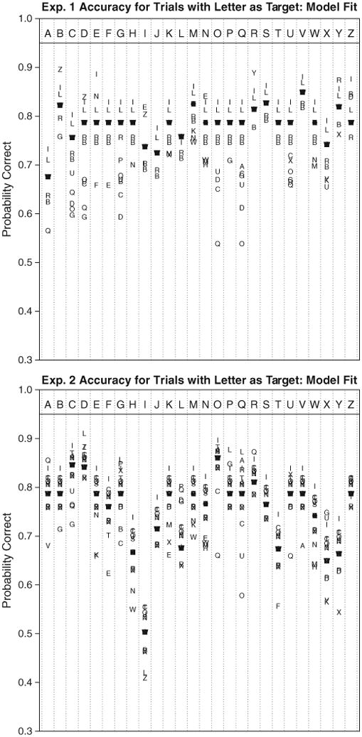
Predicted accuracy values for Experiment 1 (top panel) and Experiment 2 (bottom panel) based on the parameters of Model 3, found in Table 5.

4.2. Detailed examination of Model 3 parameters

Our comparison of models shows clear support for a similarity-free notion of perceivability, which also appears related to the similarity between the mask and the target character. Notably, perceivability for J and X were negative for both experiments: this suggests that these characters are overall difficult to identify when masked by either @ or #. The A and C were the only other characters with negative perceivability in Experiment 1, but the F, H, I, L, T, W, and Y in Experiment 2 were also reliably negative. Several characters had reliably high perceivability: M, S, V, and Y in Exp. 1, and C, D, and O in Experiment 2. Curiously, the round @ mask seemed to have little negative perceivability impact on round characters (aside from the C), whose mean recognition accuracy tended to be lower than average, but largely because of specific similarity effects between target-foil pairs.

Similarly, bias impacted performance on trials for particular targets and foils. For example, both I and L had negative bias across both experiments, coupled with negative perceivability in only Experiment 2. The overall negative bias indicated that participants were unwilling to give the letter as a response. This may stem from a miscalibrated understanding of what the perceptual evidence for these letters should have been.

Finally, the parameter search method allows variability to be explained either by experiment-specific or general target-foil similarity. Interestingly, although a large core of similar letters were identified across experiments, there were idiosyncratic similarity effects (both positive and negative) for each mask. Round characters were generally found to be similar across experiments, but the @ mask in Experiment 1 appeared to increase the similarity between D and other round letters (C, G, O, Q, U), as well as the similarity between G and Q, D, and U. Perhaps the # mask left D and G particularly easy to identify, whereas they were obscured with the @ mask. In Experiment 2, the # mask appeared to increase the similarity of A and V, F and T, H and W, and E and K. Again, the mask may have obscured or interrupted feature binding that helps discriminate between these letter pairs.

Several individual characters and character combinations stand out in this study. These include the “A” and “I” in Experiment 1, and the “X”, “H”, and “I” in Experiment 2. By examining the model parameters, we can identify psychological explanations for why these letters were identified poorly. For example, the “I” has universally negative bias across both experiments, but only has a negative perceivability in Experiment 2, where it was highly similar to features in the mask character. In other words, the # made the “I” difficult to see, but people were generally reluctant to respond with an “I”, possibly because they were miscalibrated in how difficult it actually was. While it is not surprising that the perceivabilities of the “I”, “X”, and “H” were impacted by the “#” mask, it is perhaps surprising how poor performance actually became.

The results for “A” in Experiment 1 show a similar pattern. However, this result is quite unexpected, because “A” does not seem to share low-level perceptual features with the “@”-mask. Yet the “A” still does have a strong similarity to the mask, in that the “@” mask embeds a lowercase “a” within it. This suggests that just as physical similarity between the mask and stimulus can reduce perceivability, so can more abstract similarity. This result is reminiscent to the robust finding of evidence discounting in short term priming tasks which seem to not be affected by changes in low-level visual features as long as letter identity is kept constant (Huber et al., 2001; Weidemann et al., 2005, 2008). The ubiquitous presence of the “A” letter code in the mask may have reduced the diagnosticity of evidence favoring the presence of an “A” target. This leads to a interesting question: Did the negative perceivability of “C” in Experiment 1 stem from physical interruption of features, or because of abstract letter identities? Our experiment cannot distinguish these two accounts.

The model finds that some aspects of similarity are robust for different masks, but in contrast, bias and perceivability are highly dependent on the mask. Furthermore, a number of similarity effects are sensitive to the mask as well. This suggests that the perceivability of a letter can be systematically altered via masking, but also that response biases can as well, as can the similarity of a pair of letters. We interpret these results as showing (1) the mask interferes systematically with the stimulus information, possibly both creating a partial percept and introducing additional features into the percept that must be discounted; (2) that this percept will change in similarity to both the target and the foil, producing corresponding changes in perceivability and similarity; and (3) the participant (or at least their perceptual decision system) is sensitive to these changes, and can adjust response biases in light of these perceptual changes.

4.3. Relation of our results to previous studies

It is also important to establish whether our results are broadly compatible with the numerous previous studies we identified. To make this comparison, we created a composite similarity score across eleven of the studies reported in Table 1. These included studies with uppercase letters using a variety of methods to assess confusability or similarity, including matrices reported by Banister (1927), Hodge (1962), Gibson et al. (1963), Fisher et al. (1969), Gilmore et al. (1979), Podgorny and Garner (1979; both ratings and response time data), Boles and Clifford (1989) and Gupta et al. (1983).

For each study, a composite similarity matrix was formed across the different conditions reported, so that two matrices from Townsend (1971a) were combined, two from Fisher et al. (1969) were combined, and three from Banister (1927) were combined. The exception to this practice was the rating and response time procedures of Podgorny and Garner (1979), which we dealt with separately. This formed eleven composite similarity matrices, which we then transformed into symmetric matrices by averaging each matrix with its transpose. Finally, we rank-ordered the upper-diagonal elements, with 1 indicating the most similar and 325 indicating the least similar pair, regardless of the specific measure of similarity. Bias and perceivability were not explicitly factored out using this procedure.

The eleven studies were moderately similar: inter-correlations of the cell ranks ranged between .26 and .81, with an average of .42. We then created an average matrix, which found the mean of the ranks across the eleven studies. Correlations of each individual study to the average ranged from .58 to .86, with a mean correlation of .68. The distribution of these mean ranks is plotted in Fig. 5, in order from most similar to least similar. Note that for roughly the first 100 targets, the slope is greater than 1, so that the mean rank similarity of the 100th most similar target was around 140. This is simply regression to the mean, but the fact that the mean rank similarity of the most similar pairs is fairly close their actual rank similarity (especially in contrast to the least similar pairs) indicates substantial agreement among the constituent data sets.

Fig. 5.

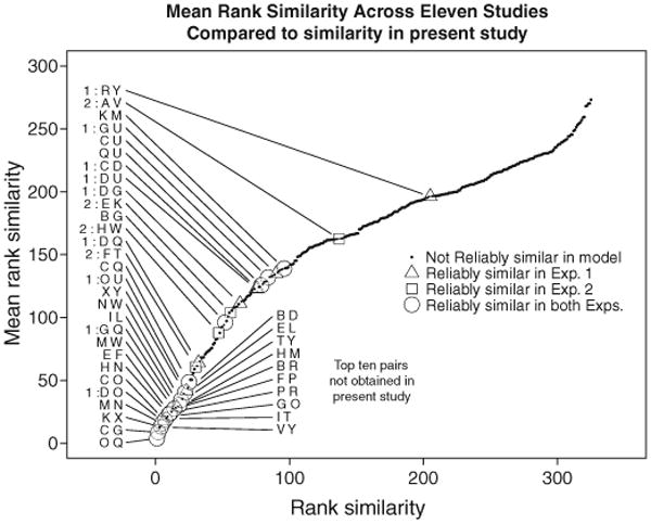
Distribution of mean of eleven rank similarities for 325 pairs of uppercase letters, along with reliable similarity parameters identified in our study. Our model tended to identify as reliably similar pairs found by these past studies to be highly similar.

Fig. 5 also shows how the reliable parameters identified by our model compare to these past studies. All but two (A–V and R–Y) of the 29 reliable similarity parameters were within the top 100 letter pairs. In addition, the figure identifies the ten most highly similar pairs (according to previous studies) that our study did not identify. These differences appear not to represent a lack of sensitivity of the model; rather, they appear to be pairs that simply were not confused disproportionately in our experiments. These differences from the past studies are most likely a consequence of the font faces and methods used to assess similarity, and possibly contamination by perceivability and bias, which were not factored out.

Our assessed similarity values (treating non-reliable values as 0) were related to the mean rank similarity values with a Pearson's ρ of .42 (t(323)=7.95; p<.001), and when adjusted so that reliable parameters tied to only one of our experiments were divided in half, the correlation rose to .46. These correlations are in the same range as the intercorrelations of the component studies that actually made up the composite score. Its lower than average correlation to the composite score stems from the fact that the other studies partly composed the composite, because bias and perceivability were not factored out of the composite scores, and because of the variety of methods and font faces were used to compute the scores. Nevertheless, this analysis shows that the parameter selection method we used was able to identify similarity parameters that are broadly in line with the similarity values identified across past studies.

4.4. Relation of our model to previous models

Our model explicitly estimates parameters associated with perceivability, bias, and similarity. Past models have typically avoided estimating all three simultaneously, but the concept does have precedent in a number of previous approaches. For example, Shepard (1957) described a model akin to choice theory that essentially went through a biased decision process twice: once for perception, and once for response. The stimulus-related weights in this model are proportional to the probability that a stimulus S is perceived if stimulus S was presented, which might be interpreted as perceivability. Interestingly, his approach was also similar to our own in that he assumed that the similarity space should be represented by a small number of parameters (identified via factor analysis instead of variable selection) which captured the major aspects of similarity.

Other subsequent research has also incorporated methods to estimate perceivability. Townsend and Landon (1983) reviewed a wide variety of models that have been used to account for confusion matrix data, and a number of those models incorporated factors that could be interpreted in terms of perceivability (especially generalized guessing models). For example, Lappin (1978) described parameters associated with both the stimulus and response space, which correspond roughly to perceivability and bias. Later, (closely following Shepard's approach) Nosofsky (1991) proposed stimulus and response biases, as well as both stimulus and response similarities, to explain confusion data. More recently, Rouder (2004) framed the variable similarity choice model (vSCM), which accounts for variability in the strength of perceivability across experimental manipulations by modulating a letter pair's similarity. Also, Massaro's 1998 Fuzzy Logical Model of Perception (FLMP) allows information from multiple distinct information channels to be combined, and if one considers similarity and perceivability as two distinct channels,² the FLMP could be viewed as enabling both similarity and perceivability to be incorporated.

Despite the numerous models that allow for concepts of perceivability, the analyses of the confusion matrices we reviewed in Table 1 frequently decomposed accuracy into just similarity and response bias, typically using the biased choice model. This approach has become popular for a number of reasons. One primary reason is because the simultaneous impact of similarity, perceivability, and bias cannot be estimated with typically approaches, and so constraints are made such that perceivability is simply equated with mean similarity. This has a primarily practical motivation, but there is theoretical sense in which this approach can be thought of as more parsimonious, because it does not require an additional theoretical concept of perceivability.

According to typical applications of the choice model to naming data (in which every letter is a potential choice alternative), the probability of making response j for a given stimulus i is:

$$p\left(j|i\right)=\frac{{\beta }_j{\eta }_{i,j}}{{\sum }_k{\beta }_k{\eta }_{i,k}},$$ (3)

where β is bias and η is similarity. The probability of correctly identifying target i with alternative j in a two-alternative forced-choice task is:

$$p_{i,j}=\frac{{\beta }_i{\eta }_{i,i}}{{\beta }_i{\eta }_{i,i}+{\beta }_j{\eta }_{i,j}},$$ (4)

In the Appendix, we show that the parameters estimated with our statistical model (λ, δ, and γ) are equivalent with transformation to corresponding parameters in choice theory. Yet in contrast to our statistical model, the choice model makes several theoretical assumptions about the nature of these factors outside our model. For example, according to choice theory, accuracy depends on the number of options being considered, and although it assumes that the relative proportion of any two responses is unaffected by the introduction of additional alternatives, the probability of making any particular response will usually be reduced by adding alternatives. Despite the fact that the choice model performs surprisingly well (Nosofsky, 1991; Smith, 1992), these assumptions have also sometimes failed to be supported by appropriate empirical tests (e.g., Ashby & Perrin, 1988; Rouder, 2001, 2004). Even though our parameter estimates can be interpreted in terms of choice theory, they do not rely on the same psychological assumptions embodied by choice theory.

Rouder's (2004) vSCM augmented choice theory by assuming the existence of an additional parameter that can be interpreted in terms of our definition of perceivability, although Rouder (2004) likely intended it as a parameter that would be applied to secondary experimental manipulations such as presentation time, and not estimated for each target stimulus. The similarities and differences between our model and the vSCM can be seen by examining a generalized version of choice theory that incorporates both our model and the vSCM (ignoring response bias for the moment), with ν corresponding to our notion of perceivability (η_i,i), s corresponding to target-foil similarity, and α corresponding to the vSCM model's notion of perceivability:

$$p\left(\nu ,s,\alpha \right)=\frac{\nu }{\nu +s^{\alpha }}$$ (5)

In the vSCM, ν = 1, whereas in our model, α = 1. The difference between the two models is that we assume perceivability impacts ν, whereas the vSCM assumes it impacts α. Because α serves to modulate s (if s is 0, α has no impact), it really serves as a modulator of similarity.

How do these assumptions fundamentally differ? Both assume that an additional parameter controls the overall chance of a stimulus being identified. In terms of our experiment (and likely most experiments we reviewed), there would probably be little difference in the resultant goodness of fit, because s would simply trade off for ν or α. However, the models do make differing predictions that may be testable. We can examine the differences by plotting how a constant change in perceivability will impact accuracy across different levels of similarity. This is illustrated in Fig. 6.

Fig. 6.

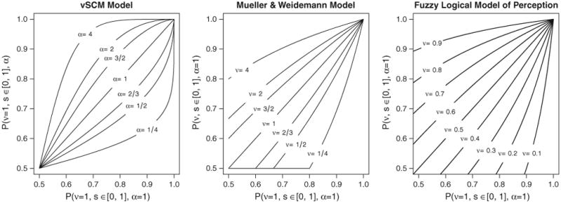
Comparison between the assumptions of our model and those of Rouder's (2004) vSCM, and Massaro's (1998) FLMP. In each panel, each line represents the accuracy obtained when perceivability is increased or decreased by a constant amount from 1.0, across a range of accuracies produced by manipulating similarity.

In Fig. 6, we began by computing a ‘baseline’ model: the range of probabilities that would be expected when both perceivability parameter was set to their default values of 1.0, and similarity was varied to produce a range of accuracies between .5 and 1.0. Then, each line represents the impact on accuracy of adjusting the perceivability parameter (α or ν) up or down from 1.0, to levels that range between 1/4 and 4. (Although equivalent values of α and ν produce value contours in similar ranges, the two parameters are not identical indices of perceivability). The models differ in several ways. First, the contours in Fig. 6 show how parametrically varying similarity should impact constant values of perceivability, and vice versa. In our model, highly-similar letters have the most to gain by increasing perceivability; in the vSCM, highly-similar letters will gain less than moderately-similar letters. Experiments testing this prediction may be possible to execute, perhaps by manipulating the choice set (and thus similarity) for a small set of characters that presumably have a constant level of perceivability across conditions. We know of no experiments that have done this, but such an experiment could provide a critical test of two distinct formalizations of perceivability in choice theory.

Another useful comparison to consider is Massaro's 1998 Fuzzy Logical Model of Perception (FLMP). Although the FLMP is designed to combine information from two distinct sources or channels (e.g., audio and visual), one might consider dissimilarity and perceivability as two distinct channels, and ask how they would interact according to the FLMP. Eq. (6) shows the basic formulation of FLMP, where a and b are probabilistic values indicating evidence from each of the two channels.

$$P_{\mathit{\text{FLMP}}}\left(a,b\right)=\frac{a\ast b}{a\ast b+\left(1-a\right)\ast \left(1-b\right)}$$ (6)

The rightmost panel of Fig. 6 shows the equivalent predictions of the FLMP. Although the input parameters are on different scales, the isosensitivity curves have a form that is quite similar to the model we propose. It could be challenging to identify an empirical test between how our model incorporates perceivability, and how the FLMP might, but both of these differ from the vSCM account.

These issues hint at some unresolved questions in the study of perception and choice. Our notion of perceivability is really quite primitive; in reality, there may be a number of factors associated with perceivability that operate differently. For example, extrinsic experimental manipulations that impact perceivability (noise, contrast, angular eccentricity, size, stimulus duration, etc.) may operate in fundamentally different ways from other more intrinsic factors that might also impact perceivability (familiarity, letter identity, letter form, font face, letter complexity, etc.). Perhaps different types of models are needed to distinguish these types of perceivabilities, such that one type of factor may map onto the vSCM approach, while the type maps onto our approach. Testing between these particular models should be possible, even though such models have been found to be very flexible and able mimic one another in many situations (cf. Pitt et al., 2003).

4.5. Relation of our results to other factors

In the past, researchers have sometimes found secondary factors that correlated with confusions or other aspects of similarity matrices. For example, one might expect response biases to favor more common letters (as would be optimal in naturalistic letter detection), and researchers have suggested that perceivability may be influenced by size or complexity of the stimuli (Attneave & Arnoult, 1956).

We examined some of these issues using the different parameters from our model. For example, we compared our estimated perceivability and bias scores to mean letter frequency (as described by Pratt, 1939). We found no reliable correlation. We also computed perimetric letter complexity via the method described by Pelli et al. (2006). This method computes a ratio between the squared perimeter of a letter and the number of black pixels in the letter, and has been shown to predict perceivability. We found no reliable correlation between these measures and our obtained perceivability scores either. These results are not too surprising, given the low correlation of these values across our two experiments–it would be difficult to be highly correlated with both sets of perceivability parameters, when they are not correlated with one another. Given that the mask has such large impacts on perceivability, there may be ways to measure complexity based on differences and similarities betweeen the mask and target, which could provide new insight into masking.

This lack of correlation can also be accounted for by the fact that Pelli et al. (2006) primarily demonstrated that mean perimetric complexity of a fontface (across the alphabet) was correlated with reduced detection efficiency and accuracy; they did not report whether differences in perimetric complexity within the characters of a font were predictive of accuracy. Their results may simply show that letters from ornate and complex font faces (which deviate from simple fonts like Helvetica) are harder to discriminate from one another (i.e., they are more similar to one another), possibly because the ornaments and serifs are specifically designed to make letters more similar to one another (see Hofstadter & McGraw, 1995).

5. Summary and conclusions

In this paper, we identified more than 70 previously published studies of alphabetic letter similarity, dating back to research conducted by Helmholtz's proteges in the 19th century. Many of these studies were perceptual detection tasks, and across experiments three primary factors have been used to account for performance: perceivability, bias, and similarity. Yet recent approaches have rarely considered all three concepts together. We conducted two experiments and developed a model that enabled us to estimate these three factors simultaneously. By doing so, we found that these three factors appear to account fairly well for our data, and in fact do so better than two-factor models incorporating only bias and similarity, with an overall more parsimonious model.

Although some early formal models incorporated factors related to perceivability, the modeling community quickly recognized the sense in which perceivability and similarity were related and could trade off, leading to the prominence of biased-choice models. One reason for this is the implicit use of balanced factorial designs to estimate parameters: there are not enough degrees of freedom to independently estimate mean values (i.e., the perceivability and bias) and the individual cells relative to that mean (i.e., the similarity effects). Thus, the notion of perceivability has essentially been abandoned in formal models of perceptual choice. This methodological limitation became an assumption of convenience and has begun to masquerade as an axiom of perception, rather than being viewed as a theory that can be tested. One of the primary conclusions of our work is that perceivability should be considered independent from mean similarity, and models should attempt to explicitly evaluate the contribution that perceivability can make.

Our model demonstrates the benefit of assuming distinct effects on bias, perceivability, and similarity. Curiously, although this approach is somewhat at odds with biased-choice theory, is actually quite consistent with the approach taken by many of the early studies we reviewed in Table 1. Studies from the 19th and early 20th centuries often focused on ranking letters with respect to “legibility”, while calling out a small number of highly-confusable letter pairs. Likewise many past studies obtained confusion matrices in which most off-diagonal cells were empty or had just a few confusions, whereas the observed confusions were concentrated in just a few pairs. Just as in this earlier research, our models identify perceivability (and bias) parameters, and a handful of similarity parameters that account for deviations from this model. Despite the current dominance of similarity and bias, we therefore believe that the study of perceptual identification in general, and that of alphabetic similarity and confusion in particular, requires careful consideration of letter perceivability.

Appendix A

Correspondence of logistic model to Luce's (1963) choice theory

For the correspondence between choice theory and our statistical model to make sense, we must make several assumptions about the meaning of different parameters which are often confounded in the application of choice theory. First, we must distinguish between a number of corresponding stimulus classes: the originally-presented distal stimuli (s_i), the perceived target (s_i), long-term perceptual memory for each letter (ŝ_i), and the perceived response alternative with little noise and strong bottom-up support (s_i). Although applications of choice theory have typically not distinguished between these, they are all in principle distinct. Whereas one might interpret the similarity parameter of choice theory as indexing a pure similarity between two abstract characters, an experiment that produced the data from which these estimates are made may actually be measuring the similarity between two different specific classes; for example, a perceived target and a long-term memory representation of that and other letters.

If λ estimates the similarity between the perceived stimulus and the correct response option (s_i and s_i), this corresponds (with appropriate transformation) to the usual interpretation of η_i,i, which is typically assumed to be 1.0. Note that this interpretation of our theory places the role of perceivability at the comparison process between the percept of the target and that of the response standard. Our bias parameters match fairly directly (with proper transformation) to their corresponding notions in choice theory, and our dissimilarity parameters are interpreted as the degree to which the percept and the response alternative match, and have a 1:1 correspondence (with transformation) to η_i,j.

As noted by others (e.g., Townsend & Landon, 1982), the more general descriptions of choice theory (e.g., Luce, 1959) express the overall probability of selecting option i from a set A based on basic logic of irrelevant alternatives: that the probability that i is chosen from A is equal to the probability that the selection option is chosen from a subset L times the probability that i would be chosen from L alone:

$$P\left(i;A\right)=P\left(L;A\right)P\left(i;L\right),$$ (A.1)

which can be expressed as:

$$P\left(i;A\right)=\frac{V\left(i\right)}{{\sum }_{j\in A}V\left(j\right)}.$$ (A.2)

Where V is the value of alternative i. Luce (1963) proposed a variation often referred to as the “biased choice model” that is suitable for N-alternative confusion matrices:

$$P_{j|i}=\frac{{\beta }_j{\eta }_{i,j}}{{\sum }_k{\beta }_k{\eta }_{i,k}},$$ (A.3)

which can be further restricted to deal with just two-alternative forced-choice accuracy:

$$P_{i,j}=\frac{{\beta }_i{\eta }_{i,i}}{{\beta }_i{\eta }_{i,i}+{\beta }_j{\eta }_{i,j}}$$ (A.4)

where η is a measure of similarity between two stimuli, and β as a response bias.

The theory (cf. Luce, 1963) makes three primary assumptions:

• Assumption 1. For all i, j ∈ S, η_{i, j} = η_{j, i}.

• Assumption 2. For all i ∈ S, η_{i, i} = 1.

• Assumption 3. For all i, j, and k ∈ S, η_{i, k} ≥ η_{i, j}η_{j, k}.

For an indirect measurement procedure such as naming, one compares the noisy percept to the perceptual memory for all letter options, and so one technically estimates η_i′,ĵ, where i′ represents the noisy percept, and ĵ represents the memory for a letter. Researchers have often assumed that η_i′,î = 1 (e.g., Townsend, 1971a, b), which is not the same as Assumption 2 of choice theory, which assumes that η_x,x = 1 for whatever x represents. In other words, Assumption 2 states that the similarity between two identical things should be 1.0, but if one is comparing a noisy memory of a letter to a clear percept of the same letter, these are not guaranteed to be identical and so it the value may be less than 1.0. Setting η_i′,ĵ = 1.0 essentially assumes the stimulus is perceived perfectly and remembered equally well.

Our statistical model is applied to a 2-AFC task, where the noisy percept (i′) is compared to two stimuli with strong perceptual support (i̅ and j). We suppose that the log-odds of a correct response p_i,j is proportional to the influence of three factors:

$$log\left(\frac{p_{i,j}}{1-p_{i,j}}\right)\propto {\lambda }_i+{\gamma }_i-{\gamma }_j+{\delta }_{i,j},$$ (A.5)

where γ is an measure of bias, λ is a measure of perceivability, and δ is a measure of dissimilarity.

By making the following substitutions into Eq. (A.5):

$${\gamma }_i=log\left({\beta }_i\right)$$

$${\lambda }_i=log\left({\eta }_{i^{\prime },\overline{i}}\right)$$

$${\delta }_{i,j}=-log\left({\eta }_{i^{\prime },\overline{j}}\right)$$

one obtains the equation

$$log\left(\frac{p_{i,j}}{1-p_{i,j}}\right)=log\left({\eta }_{i^{\prime },\overline{i}}\right)+log\left({\beta }_i\right)-log\left({\beta }_j\right)-log\left({\eta }_{i^{\prime },\overline{j}}\right).$$ (A.6)

Eq. (A.6) can be solved for p_i,j with the following intermediate steps:

$$\frac{p_{i,j}}{1-p_{i,j}}=\frac{{\beta }_i{\eta }_{i\text{'},\overline{i}}}{{\beta }_j{\eta }_{i\text{'},\overline{j}}},\frac{1-p_{i,j}}{p_{i,j}}=\frac{{\beta }_j{\eta }_{i\text{'},\overline{j}}}{{\beta }_i{\eta }_{i\text{'},\overline{i}}},\frac{1}{p_{i,j}}-1=\frac{{\beta }_j{\eta }_{i\text{'},\overline{j}}}{{\beta }_i{\eta }_{i\text{'},\overline{i}}},\frac{1}{p_{i,j}}=1+\frac{{\beta }_j{\eta }_{i\text{'},\overline{j}}}{{\beta }_i{\eta }_{i\text{'},\overline{i}}},\frac{1}{p_{i,j}}=\frac{{\beta }_i{\eta }_{i\text{'},i}+{\beta }_j{\eta }_{i\text{'},j}}{{\beta }_i{\eta }_{i\text{'},i}},p_{i,j}=\frac{{\beta }_i{\eta }_{i\text{'},i}}{{\beta }_i{\eta }_{i\text{'},i}+{\beta }_j{\eta }_{i\text{'},j}}$$ (A.7)

After applying these algebraic steps, Eq. (A.7) is identical to Eq. (A.4). Furthermore, the assumptions 1 through 3 also apply to our model. For example, we assume that similarity is symmetric (Assumption 1) and that the triangle inequality holds (Assumption 3). We also assume that the self-similarity Assumption 2 holds, but in our model perceivability is equated with a related quantity: η_i′,i̅, which is not fixed to 1.0. This quantity represents the similarity between the percept of the (masked) target and that of the correct response option. Typically, researchers have implicitly assumed that η_i′,î = 1, but this is only a technical assumption and not one based on theoretical assumptions of choice theory per se. In our model, one may still assume that η_i,i = 1, and so it does not violate Assumption 2 of choice theory.

Interpretation of our obtained parameters in terms of choice theory is straight-forward, although there is one point of caution. The obtained value δ corresponds roughly to traditional distance measures used in choice theory (cf. Luce, 1963), but our obtained measures are mostly negative, indicating high confusability. This corresponds to values of η that are greater than 1.0, but η is often constrained to be between 0 and 1, with 1.0 corresponding to “identical”. This creates a problem because if response biases are ignored, one could produce situations where response tendencies still place accuracy below 0.5 for a forced-choice task. To avoid this situation, η_i,j must be smaller than η_i,i for all i and j, which corresponds to −δ_i,j<min(λ_i,λ_j). Violations of this would indicate that choice theory provides an inadequate account of our data. This was never the case for the values of similarity and perceivability estimated in our experiments.

References

- Ashby FG, Perrin NA. Toward a unified theory of similarity and recognition. Psychological Review. 1988;95:124–150. [Google Scholar]
- Attneave F, Arnoult MD. The quantitative study of shape and pattern perception. Psychological Bulletin. 1956;53:452–471. doi: 10.1037/h0044049. [DOI] [PubMed] [Google Scholar]
- Banister H. Block capital letters as tests of visual acuity. British Journal of Ophthalmology. 1927;11:49–61. doi: 10.1136/bjo.11.2.49. [DOI] [PMC free article] [PubMed] [Google Scholar]
- Bell GL. Effects of symbol frequency in legibility testing. Human Factors. 1967;9(5):471–478. doi: 10.1177/001872086700900511. [DOI] [PubMed] [Google Scholar]
- Blommaert FJ. Early-visual factors in letter confusions. Spatial Vision. 1988;3(3):199–224. doi: 10.1163/156856888x00131. [DOI] [PubMed] [Google Scholar]
- Blough DS. Discrimination of letters and random dot patterns by pigeons and humans. Journal of Experimental Psychology: Animal Behavior Processes. 1985;11(2):261–280. doi: 10.1037//0097-7403.11.2.261. [DOI] [PubMed] [Google Scholar]
- Boles DB, Clifford JE. An upper- and lowercase alphabetic similarity matrix, with derived generation similarity values. Behavior Research Methods, Instruments, & Computers. 1989;21:579–586. [Google Scholar]
- Bouma H. Visual recognition of isolated lower-case letters. Vision Research. 1971;11:459–474. doi: 10.1016/0042-6989(71)90087-3. [DOI] [PubMed] [Google Scholar]
- Bradley RA, Terry ME. Rank analysis of incomplete block designs: I. the method of paired comparison. Biometrika. 1952;39:324–345. [Google Scholar]
- Briggs R, Hocevar DJ. A new distinctive feature theory for upper case letters. Journal of General Psychology. 1975;93(1):87–93. [Google Scholar]
- Cattell JM. Über die Trägheit der Netzhaut und des Sehcentrums. Philoso-phische Studien. 1886;3:94–127. [Google Scholar]
- Coffin S. Spatial frequency analysis of block letters does not predict experimental confusions. Perception & Psychophysics. 1978;23:69–74. doi: 10.3758/bf03214297. [DOI] [PubMed] [Google Scholar]
- Cohen AL, Sautner M. ExpLib (version 1.0.1 [beta]) 2001. [Google Scholar]
- Courrieu P, de Falco S. Segmental vs. dynamic analysis of letter shape by preschool children. Cahiers de Psychologie Cognitive/Current Psychology of Cognition. 1989;9(2):189–198. [Google Scholar]
- Craig JC. A confusion matrix for tactually presented letters. Perception & Psychophysics. 1979;26(5):409–411. [Google Scholar]
- Dawson MR, Harshman RA. The multidimensional analysis of asymmetries in alphabetic confusion matrices: evidence for global-to-local and local-to-global processing. Perception & Psychophysics. 1986;40(6):370–383. doi: 10.3758/bf03208196. [DOI] [PubMed] [Google Scholar]
- Dockeray FC, Pillsbury WB. The span of vision in reading and the legibility of letters. Journal of Educational Psychology. 1910;1:123–131. [Google Scholar]
- Dunn-Rankin P. The similarity of lowercase letters of the English alphabet. Journal of Verbal Learning and Verbal Behavior. 1968;7(6):990–995. [Google Scholar]
- Dunn-Rankin P, Leton DA, Shelton VF. Congruency factors related to visual confusion of English letters. Perceptual & Motor Skills. 1968;26:659–666. doi: 10.2466/pms.1968.26.2.659. [DOI] [PubMed] [Google Scholar]
- Engel GR, Dougherty WC, Jones GB. Correlation and letter recognition. Canadian Journal of Psychology. 1973;27(3):317–326. doi: 10.1037/h0082482. [DOI] [PubMed] [Google Scholar]
- Eriksen CW. The use of a visual mask may seriously confound your experiment. Perception & Psychophysics. 1980;28(1):89–92. doi: 10.3758/bf03204322. [DOI] [PubMed] [Google Scholar]
- Fisher DF, Monty RA, Glucksberg S. Visual confusion matrices: fact or artifact? The Journal of Psychology. 1969;71:111–125. doi: 10.1080/00223980.1969.10543077. [DOI] [PubMed] [Google Scholar]
- Gervais MJ, Harvey LO, Roberts JO. Identification confusions among letters of the alphabet. Perception & Psychophysics. 1984;10:655–666. doi: 10.1037//0096-1523.10.5.655. [DOI] [PubMed] [Google Scholar]
- Geyer LH. Recognition and confusion of the lowercase alphabet. Perception & Psychophysics. 1977;22:487–490. doi: 10.3758/bf03199550. [DOI] [PubMed] [Google Scholar]
- Geyer LH, DeWald CG. Feature lists and confusion matrices. Perception & Psychophysics. 1973;14:471–482. [Google Scholar]
- Gibson EJ. Principles of learning and development. New York: Meredith; 1969. [Google Scholar]
- Gibson EJ, Osser H, Schiff W, Smith J. A Basic Research Program on Reading: Cooperative Research Project No 639. Ithaca, NY: Cornell University; 1963. An analysis of critical features of letters tested by a confusions matrix; pp. 1–22. [Google Scholar]
- Gilmore GC, Hersh H, Caramazza A, Griffin J. Multidimensional letter similarity derived from recognition errors. Perception & Psychophysics. 1979;25:425–431. doi: 10.3758/bf03199852. [DOI] [PubMed] [Google Scholar]
- Green DM, Swets JA. Signal detection theory and psychophysics. New York: John Wiley and Sons, Inc; 1966. [Google Scholar]
- Gupta SM, Geyer LH, Maalouf JA. Effect of font and medium on recognition/confusion. Proceedings of the SIGCHI conference on Human Factors in Computing Systems. 1983:144–149. [Google Scholar]
- Hartridge H, Owen HB. Test types. British Journal of Ophthalmology. 1922;6:543–549. doi: 10.1136/bjo.6.12.543. [DOI] [PMC free article] [PubMed] [Google Scholar]
- Heiser WJ. Selecting a stimulus set with prescribed structure from empirical confusion frequencies. British Journal of Mathematical & Statistical Psychology. 1988;41(1):37–51. [Google Scholar]
- Hodge DC. Legibility of a uniform-strokewidth alphabet: I. Relative legibility of upper and lower case letters. Journal of Engineering Psychology. 1962;1:23–46. [Google Scholar]
- Hoeting J, Raftery AE, Madigan D. A method for simultaneous variable selection and outlier identification in linear regression. Computational Statistics & Data Analysis. 1996;22:251–270. [Google Scholar]
- Hofstadter D, McGraw G. Letter spirit: esthetic perception and creative play in the rich microcosm of the Roman alphabet. Ch. 10 New York, NY, USA: Basic Books, Inc; 1995. [Google Scholar]
- Huber DE, Shiffrin RM, Lyle KB, Quach R. Mechanisms of source confusion and discounting in short-term priming 2: Effects of prime similarity and target duration. Journal of Experimental Psychology: Learning, Memory, and Cognition. 2002;28:1120–1136. [PubMed] [Google Scholar]
- Huber DE, Shiffrin RM, Lyle KB, Ruys KI. Perception and preference in short-term word priming. Psychological Review. 2001;108:149–182. doi: 10.1037/0033-295x.108.1.149. [DOI] [PubMed] [Google Scholar]
- Huber DE, Shiffrin RM, Quach R, Lyle KB. Mechanisms of source confusion and discounting in short-term priming: 1. Effects of prime duration and prime recognition. Memory & Cognition. 2002;30:745–757. doi: 10.3758/bf03196430. [DOI] [PubMed] [Google Scholar]
- Jacobs AM, Nazir TA, Heller O. Perception of lowercase letters in peripheral vision: a discrimination matrix based on saccade latencies. Behavioral and Brain Sciences. 1989;46(1):95–102. doi: 10.3758/bf03208079. [DOI] [PubMed] [Google Scholar]
- Javal M. L'évolution de la typographie considérée dans ses rapports avec l'hygiène de la vue. Revue Scientifique, XXVII. 1881:802–813. [Google Scholar]
- Johnson JR, Phillips KO. Tactile spatial resolution.i.Two-point discrimination, gap detection, grating resolution, and letter recognition. Journal of Neurophysiology. 1981;46:1177–1192. doi: 10.1152/jn.1981.46.6.1177. [DOI] [PubMed] [Google Scholar]
- Keren G, Baggen S. Recognition models of alphanumeric characters. Perception & Psychophysics. 1981;29:234–246. doi: 10.3758/bf03207290. [DOI] [PubMed] [Google Scholar]
- Kikuchi T, Yamashita Y, Sagawa K, Wake T. An analysis of tactile letter confusions. Perception & Psychophysics. 1979;26(4):295–301. [Google Scholar]
- Korte W. Über die Gestaltauffassung im indirekten Sehen. Zeitschrift für Psychologie. 1923;93:17–82. [Google Scholar]
- Kuennapas T, Janson A. Multidimensional similarity of letters. Perceptual & Motor Skills. 1969;28:3–12. doi: 10.2466/pms.1969.28.1.3. [DOI] [PubMed] [Google Scholar]
- Lappin JS. The relativity of choice behavior and the effect of prior knowledge on the speed and accuracy of recognition. In: Castellan NJ, Restle F, editors. Cognitive Theory. Vol. 3. Hillsdale, NJ: LEA; 1978. [Google Scholar]
- Latecki LJ, Lakaemper R, Wolter D. Optimal partial shape similarity. Image and Vision Computing. 2005;23(2):227–236. [Google Scholar]
- Laughery KR. Computer simulation of short-term memory: a component-decay model. In: Spence JT, B GH, editors. The psychology of learning & motivation: advances in resarch and theory. Vol. 3. New York: Academic Press; 1969. pp. 135–200. [Google Scholar]
- Liu L, Arditi A. How crowding affects letter confusion. Optometry and Vision Science. 2001;78:50–55. doi: 10.1097/00006324-200101010-00014. [DOI] [PubMed] [Google Scholar]
- Loomis JM. Tactile letter recognition under different modes of stimulus presentation. Perception & Psychophysics. 1974;16:401–408. [Google Scholar]
- Loomis JM. Analysis of tactile and visual confusion matrices. Perception & Psychophysics. 1982;31:41–52. doi: 10.3758/bf03206199. [DOI] [PubMed] [Google Scholar]
- Luce RD. Individual choice behavior: a theoretical analysis. New York: Wiley; 1959. [Google Scholar]
- Luce RD. Detection and recognition. In: Luce RD, Bush RR, Galanter E, editors. Handbook of mathematical psychology. Vol. 1. New York: Wiley; 1963. [Google Scholar]
- Macmillan NA, Creelman CD. Response bias: characteristics of detection theory, threshold theory, and “nonparametric” measures. Psychological Bulletin. 1990;107:401–413. [Google Scholar]
- Macmillan NA, Creelman CD. Detection theory: a user's guide. 2nd. New York: Lawrence Erlbaum Associates; 2005. [Google Scholar]
- Majaj NJ, Pelli DG, Kurshan P, Palomares M. Role of spatial frequency channels in letter identification, the. Vision Research. 2002;42(9):1165–1184. doi: 10.1016/s0042-6989(02)00045-7. [DOI] [PubMed] [Google Scholar]
- Massaro DW. Perceiving talking faces: from speech perception to a behavioral principle. Cambridge, MA: The MIT Press; 1998. [Google Scholar]
- Mayzner MS. Studies of visual information processing in man. In: Solso TL, editor. Information Processing and Cognition: The Loyola Symposium. Hillsdale, New Jersey: L. Erlbaum Associates; 1975. [Google Scholar]
- McGraw G, Rehling J, Goldstone R, editors. Letter perception: toward a conceptual approach. Proceedings of the Sixteenth Annual Conference of the Cognitive Science Society; Atlanta, GA: The Cognitive Science Society; 1994. pp. 613–618. URL. http://citeseer.nj.nec.com/26978.html. [Google Scholar]
- Miozzo M, De Bastiani P. The organization of letter-form representations in written spelling: evidence from acquired dysgraphia. Brain and Language. 2002;80:366–392. doi: 10.1006/brln.2001.2598. [DOI] [PubMed] [Google Scholar]
- Mitchell TJ, Beauchamp JJ. Bayesian variable selection in linear regression. Journal of the American Statistical Association. 1988;83(404):1023–1032. [Google Scholar]
- Mueller ST, Weidemann CT. Decision noise: an explanation for observed violations of signal detection theory. Psychonomic Bulletin and Review. 2008;15:465–494. doi: 10.3758/pbr.15.3.465. [DOI] [PubMed] [Google Scholar]
- Myung IJ. Importance of complexity in model selection. The Journal of Mathematical Psychology. 2000;44:190–204. doi: 10.1006/jmps.1999.1283. Special Issue On Model Selection. [DOI] [PubMed] [Google Scholar]
- Myung IJ, Pitt MA. Applying occam's razor in modeling cognition: a Bayesian approach. Psychonomic Bulletin and Review. 1997;4:79–95. [Google Scholar]
- Navon D. Forest before trees: the precedence of global features in visual perception. Cognitive Psychology. 1977;9(3):353–383. [Google Scholar]
- Nosofsky RM. Stimulus bias, asymmetric similarity, and classification. Cognitive Psychology. 1991;23:94–140. [Google Scholar]
- O'Gorman TW. An adaptive method of variable selection in regression. Communications in Statistics–Simulation and Computation. 2008;37(6):1129–1142. [Google Scholar]
- Ovink GW. Legibility, atmosphere-value, and forms of printing types. Leiden, Holland: A.W. Sijthoffs Uitgeversmij N.V.; 1938. [Google Scholar]
- Paap KR, Newsome SL, McDonald JE, Schvaneveldt RW. An activation-verification model for letter and word recognition: the word-superiority effect. Psychological Review. 1982;89:573–594. [PubMed] [Google Scholar]
- Pelli DG, Burns CW, Farell B, Moore-Page DC. Feature detection and letter identification. Vision Research. 2006 Dec;46(28):4646–4674. doi: 10.1016/j.visres.2006.04.023. [DOI] [PubMed] [Google Scholar]
- Phillips JR, Johnson KO, Browne HM. A comparison of visual and two modes of tactual letter resolution. Perception & Psychophysics. 1983;34(3):243–249. doi: 10.3758/bf03202952. [DOI] [PubMed] [Google Scholar]
- Pitt MA, Kim W, Myung IJ. Flexibility versus generalizability in model selection. Psychonomic Bulletin &Review. 2003;10(1):29. doi: 10.3758/bf03196467. [DOI] [PubMed] [Google Scholar]
- Pitt MA, Myung IJ, Zhang S. Toward a method of selecting among computational models of cognition. Psychological Review. 2002;109:472–491. doi: 10.1037/0033-295x.109.3.472. [DOI] [PubMed] [Google Scholar]
- Podgorny P, Garner W. Reaction time as a measure of inter- and intraobject visual similarity: letters of the alphabet. Perception & Psychophysics. 1979;26:37–52. [Google Scholar]
- Popp HM. Visual discrimination of alphabet letters. The Reading Teacher. 1964;17:221–226. [Google Scholar]
- Pratt F. Secret and urgent: the story of codes and ciphers. Indianapolis: Bobbs-Merrill Co; 1939. [Google Scholar]
- R Development Core Team. R Foundation for Statistical Computing. Vienna, Austria: 2008. R: a language and environment for statistical computing. URL. http://www.R-project.org. [Google Scholar]
- Ratcliff R, McKoon G. A counter model for implicit priming in perceptual word identification. Psychological Review. 1997;104:319–343. doi: 10.1037/0033-295x.104.2.319. [DOI] [PubMed] [Google Scholar]
- Ratcliff R, McKoon G, Verwoerd M. A bias interpretation of facilitation in perceptual identification. Journal of Experimental Psychology: Learning, Memory, and Cognition. 1989;15:378–387. doi: 10.1037//0278-7393.15.3.378. [DOI] [PubMed] [Google Scholar]
- Reich LN, Bedell HE. Relative legibility and confusions of letter acuity in the peripheral and central retina. Optometry and Vision Science. 2000;77(5):270–275. doi: 10.1097/00006324-200005000-00014. [DOI] [PubMed] [Google Scholar]
- Roethlein BE. The relative legibility of different faces of printing types. American Journal of Psychology. 1912;23:1–36. [Google Scholar]
- Rouder JN. Absolute identification with simple and complex stimuli. Psychological Science. 2001;12:318–322. doi: 10.1111/1467-9280.00358. [DOI] [PubMed] [Google Scholar]
- Rouder JN. Modeling the effects of choice-set size on the processing of letters and words. Psychological Review. 2004;111:80–93. doi: 10.1037/0033-295X.111.1.80. [DOI] [PubMed] [Google Scholar]
- Sanford EC. The relative legibility of the small letters. American Journal of Psychology. 1888;1:402–435. [Google Scholar]
- Schwarz G. Estimating the dimension of a model. Annals of Statistics. 1978;6:461–464. [Google Scholar]
- Shepard RN. Stimulus and response generalization: a stochastic model relating generalization to distance in psychological space. Psychometrika. 1957;22:325–345. doi: 10.1037/h0042354. [DOI] [PubMed] [Google Scholar]
- Smith JEK. Alternative biased choice models. Mathematial Social Sciences. 1992;23:199–219. [Google Scholar]
- Thorson G. An alternative for judging confusability of visual letters. Perceptual & Motor Skills. 1976;42(1):116–118. doi: 10.2466/pms.1976.42.1.116. [DOI] [PubMed] [Google Scholar]
- Tinker MA. The relative legibility of the letters, the digits, and of certain mathematical signs. Journal of General Psychology. 1928;1:472–496. [Google Scholar]
- Townsend JT. Theoretical analyses of an alphabetic confusion matrix. Perception & Psychophysics. 1971;9:40–50. [Google Scholar]
- Townsend JT. Alphabetic confusion: a test of models for individuals. Perception & Psychophysics. 1971;9:449–454. [Google Scholar]
- Townsend JT, Landon DE. An experimental and theoretical investigation of the constant-ratio rule and other models of visual letter confusion. Journal of Mathematical Psychology. 1982;25(2):119–162. [Google Scholar]
- Townsend JT, Landon DE. Mathematical models of recognition and confusion in psychology. International Journal of Mathematical Social Sciences. 1983;4:25–71. [Google Scholar]
- Uttal WR. Masking of alphabetic character recognition by dynamic visual noise (DVN) Perception & Psychophysics. 1969;6:121–128. [Google Scholar]
- van der Heijden AHC, Malhas MS, van den Roovart BP. An empirical interletter confusion matrix for continuous-line capitals. Perception & Psychophysics. 1984;35:85–88. doi: 10.3758/bf03205927. [DOI] [PubMed] [Google Scholar]
- van Nes FL. New characters for Teletext with improved legibility. IPO Annual Progress Report. 1983;18:108–113. [Google Scholar]
- Venables WN, Ripley BD. Modern applied statistics with S. 4th. New York: Springer; 2002. [Google Scholar]
- Watson AB, Fitzhugh AE. Modelling character legibility. Society for Information Display Digest of Technical Papers. 1989;20:360–363. [Google Scholar]
- Weidemann CT, Huber DE, Shiffrin RM. Confusion and compensation in visual perception: effects of spatiotemporal proximity and selective attention. Journal of Experimental Psychology: Human Perception and Performance. 2005;31:40–61. doi: 10.1037/0096-1523.31.1.40. [DOI] [PubMed] [Google Scholar]
- Weidemann CT, Huber DE, Shiffrin RM. Prime diagnosticity in short-term repetition priming: is primed evidence discounted, even when it reliably indicates the correct answer? Journal of Experimental Psychology: Learning, Memory, and Cognition. 2008;34:257–281. doi: 10.1037/0278-7393.34.2.257. [DOI] [PubMed] [Google Scholar]
- Yamashita T, Yamashita K, Kamimura R. A stepwise AIC method for variable selection in linear regression. Communications in Statistics–Theory and Methods. 2007;36:2395–2403. [Google Scholar]