A quantum–quantum Metropolis algorithm

Abstract

The classical Metropolis sampling method is a cornerstone of many statistical modeling applications that range from physics, chemistry, and biology to economics. This method is particularly suitable for sampling the thermal distributions of classical systems. The challenge of extending this method to the simulation of arbitrary quantum systems is that, in general, eigenstates of quantum Hamiltonians cannot be obtained efficiently with a classical computer. However, this challenge can be overcome by quantum computers. Here, we present a quantum algorithm which fully generalizes the classical Metropolis algorithm to the quantum domain. The meaning of quantum generalization is twofold: The proposed algorithm is not only applicable to both classical and quantum systems, but also offers a quantum speedup relative to the classical counterpart. Furthermore, unlike the classical method of quantum Monte Carlo, this quantum algorithm does not suffer from the negative-sign problem associated with fermionic systems. Applications of this algorithm include the study of low-temperature properties of quantum systems, such as the Hubbard model, and preparing the thermal states of sizable molecules to simulate, for example, chemical reactions at an arbitrary temperature.

Interacting many-body problems cover a wide range of applications in many areas in science and technology. These are best exemplified by the Ising spin model, which was originally developed for explaining ferromagnetism and its associated phase transitions (1). The Ising model was later found to be related to many practical applications, for example, error-correcting codes, image restoration, associative memory, and optimization problems (see, e.g., ref. 2). However, there is no efficient method for finding solutions to many-body problems in general. For example, the problem of finding the ground state of the Ising model with arbitrary couplings is known to be a nondeterministic polynomial (NP)-complete problem, meaning that, if an efficient algorithm for solving the Ising model exists, then all of the problems in the class of NP, for example the graph isomorphism problem and some variants of the traveling salesman problem, can be solved efficiently as well (see, e.g., ref. 3).

The most fundamental challenge for solving many-body problems is that they generally require an exponentially large amount of spatial and temporal computing resources to find the solutions as the system size increases (4). Although no universal method for solving general many-body problems has been found, powerful classical methods such as Markov-chain Monte Carlo (MCMC) or quantum Monte Carlo (QMC) have been invented and proven to be successful in many applications (see, e.g., ref. 5). These methods, however, have certain limitations. For example, the running time of MCMC scales as O(1/δ) (6), where δ is the gap of the transition matrix. For problems such as spin glasses (7) where δ is vanishingly small as a function of system size, MCMC becomes computationally inefficient. QMC methods, on the other hand, suffer from the negative-sign problem (8), making them inefficient for problems involving fermions, e.g., electronic problems. Despite the many efforts toward improvement that have been made (9), this limitation is still one of the biggest challenges in QMC (10).

Background of Quantum Simulation

One of the most important goals in the field of quantum computation, as proposed by Feynman (11), is to look for methods or algorithms that can solve these many-body problems more efficiently. A promising solution is quantum simulation, which aims at employing a controllable quantum system to simulate the behaviors of the target quantum system. Quantum simulation can solve the problem of the spatial requirement for solving many-body problems. Quantum simulation can be implemented either by dedicated (or analog) quantum simulators (12) or with universal (or digital) quantum computers (13). For analog quantum simulation, high-precision experimental techniques are required for faithful simulation, and therefore involves many engineering challenges. An example is the use of neutral atoms trapped in optical lattices (14) to simulate the low-temperature properties of the Hubbard or Bose–Hubbard model.

Digital Quantum Simulation.

To look for algorithms based on the special properties of the laws of quantum mechanics, top-down approaches aim to improve the existing classical algorithms by combining them with elementary quantum algorithms. For the bottom-up approach, in the context of quantum simulation, the only known example that quantum algorithms can achieve exponential gain over classical methods is the simulation of time dynamics (15, 16). It was also discovered (17) that such an approach is particularly suitable for simulating single or many-particle systems where the Hamiltonians consist of two terms, namely kinetic energy and potential energy, for example, atomic or molecular systems (18). On the other hand, however, attempt to create quantum algorithms to solve the ground-state (19, 20) or thermal-state (21–23) problems of unstructured Hamiltonians failed to show an exponential gain over classical approaches. However, this lack of an exponential advantage does not mean that quantum computers fail to show advantages over classical computers in quantum simulation.

Variational Methods.

In fact, many problems in physics and chemistry do exhibit certain symmetries or structures. These features allow us to take the top-down approach to generalize methods that are proven to be successful in classic computing to design quantum algorithms. For example, the variational wavefunctions, such as the Bardeen–Cooper–Schrieffer wavefunction in superconductivity and the Hartree–Fock solutions in the electronic problems of atomic and molecular systems, are good approximations to the exact ground states of the corresponding Hamiltonians to some extent. With the quantum phase estimation algorithm (24, 25), it is possible to project the exact ground states from the approximate solutions with high probabilities. Further theoretical investigations on the efficiency of this method on molecular systems have been made (26–28), and a related experimental implementation has been realized (29).

Markov-Chain-Based Methods.

For problems where clever approximating solutions are unavailable, one may still be able to solve them efficiently by using Markov-chain-based Monte Carlo methods. In the context of quantum computation, Szegedy described a method to quantize classical Markov chains (30). The key result is that a quadratic speedup in the gap δ of the transition matrix is possible. This idea was later adapted to other algorithms (31, 32) for preparing thermal states of classical Hamiltonians, based on the idea of quantum simulated annealing (QSA) (31).

In fact, Markov chains that correspond to classical Hamiltonians are relatively easy to construct, as all the eigenstates of classical Hamiltonians are in the computational basis . However, preparation of the thermal states of quantum Hamiltonians (20, 21, 33, 34), where the eigenvectors are in nontrivial superposition of the computational basis vectors, is a much more challenging problem for classical computation. Classically, one would need to solve for the full eigenvalue problem (i.e., look for all eigenvalues and eigenvectors) for the quantum Hamiltonian first, which often requires more computational resources than directly computing the corresponding partition functions. Quantum mechanically, any attempt for a straightforward generalization of the classical method by Szegedy would encounter the problem due to the inability to clone quantum states (35).

Quantum Metropolis Methods.

The key strategy that has been employed so far to overcome the difficulty of obtaining information about eigenvectors of quantum Hamiltonians with a quantum computer is the use of the quantum phase estimation algorithm (24); the eigenvalues of a quantum Hamiltonian can be recorded without explicitly knowing the detailed structure of the eigenvectors. Based on this idea, Terhal and DiVincenzo (33) made an attempt to extend the Metropolis algorithm (5) to the quantum domain in order to avoid the negative-sign problem in QMC. However, one limitation of their result is that the key step involves too many energy nonlocal transitions, making it inefficient for solving practical problems. Recently, Temme et al. (34) addressed this problem by introducing a measurement-based rejection method, which makes the algorithm more realistic for simulating many-body problems. This result shows that quantum computers can solve many-body problems beyond the limits of classical computers. However, the underlying Markov chains of this algorithm are still classical in nature, which means that the scaling of the running time is still O(1/δ).

Motivation, Results, and Outline of the Quantum–Quantum Metropolis Algorithm (Q²MA)

To summarize, before this work, the existing quantum algorithms were capable of either (i) preparing thermal states of classical systems with quantum speedup (31, 32), or (ii) preparing thermal states of quantum systems without quantum speedup (33, 34); this suggests that the potential of quantum computers may not have been fully exploited. This problem motivates us to further explore the power of quantum computation by providing a quantum algorithm that allows us to prepare thermal states of quantum systems with quantum speedup.

Instead of following the path developed in the work of Temme et al. (34), we took the following strategy: First of all, a natural question to ask is whether Szegedy’s quantum speedup is restricted to employing classical Hamiltonians, where the eigenstates simply coincide with the computational basis, making cloning of the classical information possible. In this manuscript, we extend the Szegedy approach to be able to deal with quantum Hamiltonians; we introduce a quantum version of the method of Markov-chain quantization which is combined with the QSA procedure (31). Formally, we propose a quantum Metropolis algorithm that exhibits a quadratic quantum speedup as a function of the eigenvalue gap δ of the corresponding Metropolis Markov matrix M for any quantum Hamiltonian H. Note that, because classical Hamiltonians belong to a subclass of quantum Hamiltonians, our algorithm is also applicable to classical systems.

Lastly, we note that this algorithm is still limited by the Markov-chain gap δ, which implies that there are problems, especially ground-state problems of frustrated systems, where this algorithm cannot solve efficiently. This result is expected, as otherwise, hard problems (20) in the quantum Merlin–Arthur complexity class (and even NP) would be solved by this algorithm. Whether such a quantum algorithm could exist is still one of the major open questions in quantum information science.

Summary of the Main Results.

The quantum Metropolis algorithm constructs the thermal state, ρ_th = e^-βH/Tr(e^-βH), for any given quantum (or classical) Hamiltonian H, where the system to be simulated is prepared at a given temperature T (β ≡ 1/k_BT), with a quadratic quantum speedup in the gap δ of the corresponding Markov matrix M. We call this Q²MA because it shows a quantum speedup for the Markov chain of thermal-state preparation for a quantum system being simulated. For comparison, the construction method by Temme et al. (34) is restricted by the no-cloning theorem insofar as the information of a eigenstate cannot be retrieved after accepting the proposed move in the Metropolis step. We relax this restriction by adopting a dual representation where the basis states consist of pairs of eigenstates related by time-reversal operation (see Eq. 8). For the cases where the physical system being simulated is time-reversal invariant, the pair of the eigenstates forming the basis vector become identical. This construction effectively circumvents the restriction imposed by the no-cloning theorem.

Outline of the Key Ideas of Q²MA.

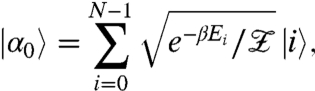
The goal of the proposed Q²MA is to prepare the coherent encoding of the thermal state (CETS),

[1]

where 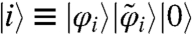, the state is the eigenstate of a quantum Hamiltonian H, associated with the eigenvalue E_i, and is the partition function. The state is the time-reversal counterpart (complex conjugate) of , which is the eigenstate of the corresponding time-reversal Hamiltonian with the same eigenenergy E_i. After tracing out all of the ancilla quantum bits (qubits), the CETS is equivalent to 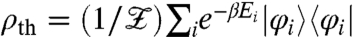. An outline of this algorithm is shown in Fig. 1. The steps go as follows: A maximally entangled state is the input state of the algorithm. Alternative input states are possible as long as they have a finite overlap with the CETS, but for simplicity we will focus on only one particular type of input state here. This maximally entangled state can be mathematically transformed into a state (see Eq. 8) that spans the dual basis related to the Hamiltonian H to be simulated. Note that this state represents the infinite temperature β = 0 state. Next, a generalization of Szegedy’s operator W (see Eq. 12) will be constructed and applied to the input state. The main purpose of W is to project out the CETS at a lower temperature through the quantum phase estimation algorithm. A similar procedure is then repeated for projecting out a CETS at an even lower temperature, and so on. The whole procedure for “adiabatically” preparing from a high-temperature CETS to a lower-temperature one is known as QSA (31). When the ancilla qubits are traced out, we obtain the thermal density matrix ρ_th = e^-βH/Tr(e^-βH), which accomplishes the goal of the Q²MA.

Fig. 1.

Outline of the Q²MA for preparing thermal states of quantum Hamiltonians H. (i) A maximally entangled state, , of n qubits is first prepared. (ii) Then, it is mathematically transformed into a maximally entangled state, (see Eq. 8), associated with the Hamiltonian H. (iii) A schedule of QSA (31) is then applied to this state, lowering the simulated inverse temperature from zero to β. The QSA algorithm is based on the phase estimation algorithm using the Szegedy operator W defined in Eq. 12. (iv) The resulting state is a CETS described in Eq. 1. (v) The final state becomes the thermal state ρ = e^-βH/Tr(e^-βH), after tracing out all of the ancilla qubits.

Organization of the Paper.

We first summarize the features of Markov chains, Metropolis sampling, and Szegedy’s method that are related to this work, in a way that become applicable to both classical and quantum systems. Next, we outline the generalization of the method of Markov-chain quantization by Szegedy (30) to make it applicable to quantum Hamiltonians H. Then, we analyze the structure of the Szegedy operator W in detail. Finally, we combine the results above with the method of quantum simulated annealing (31) to generate thermal states of quantum systems at any finite temperature T. We describe nonessential technical details in the SI Text.

Review of the Classical Metropolis Method

In the standard Metropolis scheme as employed in classical computation (5), the thermal Gibbs distribution of certain a eigenstate of a certain Hamiltonian H, associated with the eigenenergy E_i, at an inverse temperature β = 1/k_BT, is generated through a Markov-chain procedure, in which the matrix element m_ij of the corresponding Markov transition matrix M refers to the transition probability from the eigenstate to . The equilibrium (stationary) distribution of the Markov-chain procedure, , satisfies the following detailed balance condition:

[2]

For classical Hamiltonians, the eigenstate vector is simply one of the vectors in the computational basis , but for quantum Hamiltonians, is, in general, a nontrivial superposition of the computational basis vectors.

The Metropolis Filter.

The Metropolis method solves problems by using an efficient way to construct a Markov chain so that the final distribution of certain random variables is identical to the distribution {π_i}. A well-known solution that can satisfy the detailed balance condition [2] is given by the following choice: m_ji = s_ijz_ji, where s_ij = s_ji is any symmetrical transition probability, and

[3]

is sometimes called the Metropolis filter, which determines the acceptance or rejection of a proposed change of the eigenstates by comparing the energy difference between them.

In a practical implementation of the Metropolis method (e.g., when applied to the Ising model), one starts with an arbitrary initial configuration of spins and then applies a random transition (e.g., single spin-flip) from one configuration (eigenstate) to another, and compares the energy between the new eigenstate and the old one. According to the rule in Eq. 3, if the new eigenstate has a lower energy, then the move is accepted. Otherwise, the move is accepted only with a probability distribution given by the ratio of the corresponding Boltzmann factors—i.e., e^-β(E_j-E_i). It is important to note that, in the whole operation, the explicit knowledge of the partition function , which usually cannot be computed efficiently, is not required.

Performance of the Metropolis Method.

The performance of the Metropolis method depends on many factors. For many cases, it depends on the properties of the underlying transition matrix M of the Markov chain, especially the eigenvalues λ_k, which are all positive and bounded by one, and the largest eigenvalue is always equal to one. For convenience, we order them as λ₀ = 1 > λ₁≥⋯≥λ_N-1 > 0. The problem is solved when the Markov-chain procedure produces the stationary distribution {π_i}. The convergence time of a Markov chain is limited by the eigenvalue gap δ ≡ 1 - λ₁ of the transition matrix M as O(1/δ) (6). For problems such as spin glasses (7), this gap can be very small, and hence it will necessarily take a long time to solve. The purpose of this work is to show that the running time of quantum algorithms can be improved to , and that we can fully extend the Metropolis sampling algorithm into the quantum domain (i.e., for quantum Hamiltonians and with quantum speedup).

Summary of Szegedy’s Method

The idea of Szegedy’s method (30) of Markov-chain quantization is to construct a unitary operator W that contains the information of a Markov matrix, which turns out to have two important properties: (i) the CETS of Eq. 1 is one of the eigenstates of W, and (ii) the eigenvalue gap scales . These two properties are important for generating classical thermal states through annealing (31, 32).

The first step of Szegedy’s method is to encode the information about the transition matrix elements m_ij into a pair of unitary operators, which acts on two sets of qubits:

[4]

[5]

where and are state vectors in the computational basis. Let us define a more compact notation . Using the detailed balance condition in Eq. 2, we have , which implies that, within the subspace , the matrix is therefore a similar matrix to the Markov matrix M (i.e., same eigenvalue spectrum {λ_k}). Based on this property, the Szegedy operator is defined as

[6]

where is the identity operator, , and . Now define a set of eigenvectors such that . By direct substitution, the Szegedy operator is block diagonal and can be decomposed into 2 × 2 matrices in the subspace :

[7]

where cos θ_k ≡ λ_k. For k = 0 (i.e., λ₀ = 1), we have , where contains the stationary distribution of the Markov chain (see SI Text), which is point (i) above. On the other hand, the eigenvalues of w_k are exp( ± 2iθ_k), and the eigenvalue gap Δ ≡ |1 - e^2iθ₁| satisfies the following inequality: , which corresponds to point (ii) and leads to the quadratic speedup (31, 32).

Generalization of the Markov-Chain Quantization Method to Quantum Hamiltonians

The Markov-chain quantization method by Szegedy (30) discussed above is applicable to classical Hamiltonians only, because it was formulated in the computational basis. To extend Szegedy’s method to make it applicable to quantum Hamiltonians, we start with the following procedure: first we prepare a set of n qubits initialized in the state , or equivalently , where N = 2ⁿ. By performing a bit-by-bit controlled-NOT gate on a set of n ancilla qubits initialized in the state , we obtain the maximally entangled state , which can be formally expressed as an entangled state of the form (SI Text)

[8]

where is an energy eigenstate of H (i.e., ), and is the time-reversal counterpart (complex conjugate) of , which is the eigenstate of the corresponding time-reversal Hamiltonian with the same eigenenergy E_i (i.e., ). As we shall see, the pair structure of the eigenvectors provides a unique feature for our construction of the quantum algorithm. For example, through the phase estimation algorithm (PEA), the value of eigenvalue E_i can be obtained either from or ; this is the key property introduced in this paper, which relaxes the constraints of the previous quantum Metropolis algorithm (34) in applying it to Szegedy’s method.

In the following, for the purpose of clarity, we shall assume that the PEA can be applied perfectly, in the sense that each eigenstate can be uniquely identified by a unique eigenvalue. It turns out that the problem of degeneracy of the eigenenergies of a quantum Hamiltonian alone is not necessarily a hurdle for the construction of our algorithm. We leave our discussion on the effects of degeneracy on this algorithm to the SI Text.

Encoding the Information of the Markov Chain.

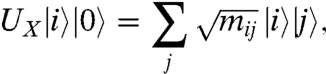
We have prepared the initial input state [8] of the Q²MA. Now, we have to define the required operations: Let us include in our Hilbert space an extra qubit initialized in the state and define a more compact notation, . In the Q²MA, the information of a Markov chain (i.e., z_ij) is encoded in a pair of unitary operators U_X and U_Y in the following way (see Eqs. 4 and 5, and see SI Text for their detailed construction):

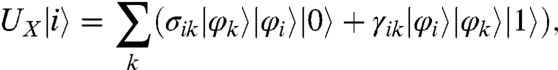[9]

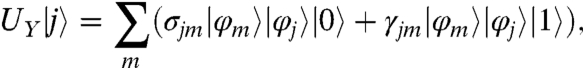[10]

where , , and . Here, K is an unitary operator, and like the spin-flip operator σ_x in the classical Metropolis method, K causes transitions from one eigenstate to another. Here, z_ik is the Metropolis filter defined in Eq. 3. Note that U_Y is related to U_X by a controlled-SWAP operation.

The physical meaning of U_X is that, when the system is in the eigenstate , the transition probability for it to make a transition to another eigenstate is |σ_ik|² ∝ z_ik. This operation is consistent with the rules in the classical Metropolis method. The meaning of U_Y is not as clear as U_X; the way U_Y is constructed is mainly to make the combination contain the same eigenvalue spectrum as the Markov matrix M (see Eq. 11).

Connection with the Markov Matrix.

To see an explicit connection between the operators U_X and U_Y with the Metropolis Markov matrix M, we will apply the detailed balance condition [2] to the product of and U_Y, which are the key elements in constructing Szegedy’s operator W (Eq. 12). From Eqs. 9 and 10, for j ≠ i, we have , where we used . Note that the right-hand side is equal to (m_ijm_ji)^1/2. On the other hand, , which, as we shall see, can be interpreted as the probability of not undergoing a transition. Now, using Eq. 2, we obtain the following decomposition:

[11]

where is a diagonal matrix, and , with and for j ≠ i, is the transition matrix of the Markov chain. Within the subspace , Eq. 11 implies that and M are similar matrices, which means that they have the same set of eigenvalues λ_k. The stationary distribution of M is the same as the Gibbs distribution for the quantum system to be simulated. This property is relevant to the construction of Szegedy’s operator W, which is defined in the following section.

Construction of the Generalized Szegedy Operator

Now, we have shown in Eq. 11 that the product is a similarity transform of a Markov matrix M within the subspace . We will need to take one more step to see how this property can lead us to be able to make good use of it. Following Szegedy (30), the results above allow us to construct a unitary operator (see Eq. 6)

[12]

where is the identity operator, and the two projectors are defined by and . Note that the structure of W is similar to those reflectors in other Grover-type algorithms. It therefore comes as no surprise that one can achieve a quadratic quantum speedup. However, the quantum speedup achieved here is quite different from that in the Grover-search problem, where the quantum speedup refers to the gain in the reduction of computational steps compared with the problem size. Here, the quantum speedup refers to the gain in the amplification of the Markov gap from δ to , which has no direct relationship with the problem size.

Spectral Properties of the Generalized Szegedy Operator.

The Szegedy operator W will be employed to perform the projection of the CETS (see Eq. 1) in the phase estimation algorithm. In the following, we will show that the “ground state” of W is indeed the CETS. The spectral properties of W can be seen in the following way: Define to be the eigenvectors of ; the eigenvalue equation can be written as . On the other hand, using the fact (see SI Text) that , we have . These two equations suggest that, if we start with vectors within Λ₁, W can be block-diagonalized into subspace of 2 × 2 matrices w_k spanned by the basis . Explicitly (see Eq. 7),

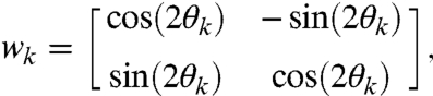
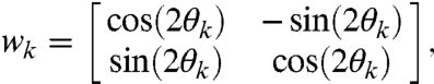[13]

where cos θ_k ≡ λ_k. Note that the eigenvalues of w_k is e^±iθ_k. In the case of k = 0, where λ₀ = 1 (or θ₀ = 0), is simply an identity matrix.

From Eq. 11 and the properties of the Markov matrix (see details in SI Text), the k = 0 state is the CETS in Eq. 1. Recall that , the state becomes the Gibbs thermal state ρ_th = e^-βH/Tr(e^-βH) when the other qubits are traced out.

Quadratic Quantum Speedup.

One of the most important features about W is that the minimum eigenvalue gap Δ_min ≡ |2θ₁| of W is larger than two times the square root of the gap δ ≡ 1 - λ₁ of the transition matrix M (using ):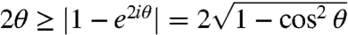

[14]

which is the mathematical origin of the quadratic speedup of Szegedy’s algorithm. Recall that, for classical Markov-chain algorithms, the performance scales as O(1/δ) (6). As we shall see next, when we apply W in the phase estimation algorithm, the performance scales as .

This section completes our discussion on the necessary tools needed for the following discussion, and we are ready to go through the method of QSA (31).

Quantum Simulated Annealing

Our quantum simulation algorithm goes as follows: Given a quantum Hamiltonian H and any finite temperature T, the goal is to obtain the corresponding CETS of the form in Eq. 1, from the initial state defined in Eq. 8, which can be readily prepared from the state , and which can be considered as the infinite-temperature (β = 0) state. To achieve this goal, we can use the method of QSA (31). For completeness, we outline the basic strategy and summarize the related results in the following paragraph. Technical details are included in the SI Text.

Let us suppose that we aim to obtain the CETS corresponding to the temperature β. The strategy of the QSA method is to prepare a sequence, j = 0,1,2, ..,d, of d + 1 of coherent thermal states, 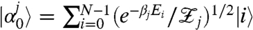, at a time; the temperature β_j ≡ (j/d)β of the coherent thermal state is lowered in each step. The basic idea for implementing this procedure is that, for a sufficiently small change of β, Δβ ≡ β/d, one can show that the CETS has a good overlap with another CETS at a lower temperature. Explicitly, the fidelity between the two states is bounded by the following expression: , where ϵ₀ is bounded by O(Δβ²∥H∥²) (SI Text).

The next step in the QSA is to consider a projective measurement operator constructed in the eigenbasis of . When Π_k+1 is applied to the CETS , it will result in the lower-temperature state with a high probability. The same procedure is then repeated for the other CETS at lower temperatures. For the entire process,

[15]

The total error accumulated (see details in SI Text) ϵ = dϵ₀ < O(β²∥H∥²/d) can be suppressed by refining the step size, which is analogous to the quantum Zeno effect applied to a slowly varying basis.

Now, using the machinery we have developed, the operator* W_j+1 can be used to construct such a projective measurement, through the phase estimation algorithm (32) (see also SI Text). Alternatively, one may employ the method in ref. 31, which is equivalent to some projective measurements, where W_j+1 is applied multiple times randomly. In any case, the number of controlled W_j+1 is at most for each step of annealing, which is a quadratic speedup relative to classical Markov chains.

Comparison with Other Related Quantum Algorithms

To summarize, we have described a quantum Metropolis algorithm that extends Szegedy’s method of classical Markov-chain quantization to the quantum domain and provides a quadratic quantum speedup in the gap δ of the transition matrix M. This extension is achieved by adopting a dual representation where the set of basis states consists of pairs of eigenstates related by the time-reversal operation. The algorithm requires twice the amount of system qubits, and the number of ancilla qubits has a logarithmic dependence on temperature O[log(1/T)]. Details for comparison are summarized in the SI Text.

A comparison of various Markov-chain-based quantum algorithms is summarized in Table 1. To facilitate reading, we explain several definitions and terminologies below: (i) the term “classical Hamiltonian” (e.g., Ising spin model) refers to the cases where the eigenstates are the same as the basis states in the computational basis; the term “Quantum Hamiltonians” refer to the cases where the eigenstates generally contain superposition states of the states in the computational basis. Therefore, the eigenstates of the classical Hamiltonians are by definition known, whereas those for quantum Hamiltonians are not. (ii) The symbol ρ refers to a density matrix, , and the quantum state as defined by Eq. 8). (iii) The thermal density matrix is ρ_th = e^-βH/Tr(e^-βH), CETS II is defined in Eq. 1), and CETS I (see also ref. 23) is similar to CETS II, but the basis states are replaced by the computational basis. (iv) By “quantum speedup”, we consider only the quantum speedup with respect to the gap δ of the transition matrix of the Markov chain. It is not known whether other types of quantum speedup exist.

Table 1.

Comparison of various Markov-chain-based algorithms for thermal-state preparation (see text for definitions)

Methods	Hamiltonian	Input	Output	Quantum speedup
Q Metropolis I (33)	quantum	any ρ	ρth	no
Q Metropolis II (34)	quantum	any ρ	ρth	no
Q Markov chain I (31)	classical		CETS I	quadratic
Q Markov chain II (32)	classical		CETS I	quadratic
Q2MA (this work)	quantum		CETS II	quadratic

Conclusion

In conclusion, we presented a quantum algorithm that completes the generalization of the classical Metropolis method to the quantum domain. Similar to ref. 34, the advantages of this quantum algorithm over classical algorithms can be exponential because there is no need to explicitly solve for the eigenvalues and eigenvectors using classical algorithms for the quantum Hamiltonians being simulated. Finally, as the application of the Metropolis method to quantum Hamiltonians can be considered as a special case of quantum maps (operations), it may be possible that the results presented here could be generalized to allow quantum speedup for a much broader class of quantum maps.

References

- 1.Brush SG. History of the Lenz-Ising model. Rev Mod Phys. 1967;39:883–893. [Google Scholar]
- 2.Nishimori H. Statistical Physics of Spin Glasses and Information Processing: An Introduction. Oxford: Oxford Univ Press; 2001. [Google Scholar]
- 3.De las Cuevas G, Dür W, Van den Nest M, Martin-Delgado MA. Quantum algorithms for classical lattice models. New J Phys. 2011;13:093021. [Google Scholar]
- 4.Kohn W. Nobel Lecture: Electronic structure of matter—wave functions and density functionals. Rev Mod Phys. 1999;71:1253–1266. [Google Scholar]
- 5.Thijssen JM. Computational Physics. Cambridge, UK: Cambridge Univ Press; 1999. [Google Scholar]
- 6.Aldous DJ. Some inequalities for reversible Markov chains. J London Math Soc. 1982;s2-25:564–576. [Google Scholar]
- 7.Mezard M, Parisi G, Virasoro MA. Spin Glass Theory and Beyond. Teaneck, NJ: World Scientific; 1987. [Google Scholar]
- 8.Troyer M, Wiese U-J. Computational complexity and fundamental limitations to fermionic quantum Monte Carlo simulations. Phys Rev Lett. 2005;94:170201–170204. doi: 10.1103/PhysRevLett.94.170201. [DOI] [PubMed] [Google Scholar]
- 9.Kalos M, Pederiva F. Exact Monte Carlo method for continuum fermion systems. Phys Rev Lett. 2000;85:3547–3551. doi: 10.1103/PhysRevLett.85.3547. [DOI] [PubMed] [Google Scholar]
- 10.Foulkes W, Mitas L, Needs R, Rajagopal G. Quantum Monte Carlo simulations of solids. Rev Mod Phys. 2001;73:33–83. [Google Scholar]
- 11.Feynman RP. Simulating physics with computers. Int J Theor Phys. 1982;21:467–488. [Google Scholar]
- 12.Buluta I, Nori F. Quantum simulators. Science. 2009;326:108–111. doi: 10.1126/science.1177838. [DOI] [PubMed] [Google Scholar]
- 13.Kassal I, Whitfield JD, Perdomo-Ortiz A, Yung M-H, Aspuru-Guzik A. Simulating chemistry using quantum computers. Annu Rev Phys Chem. 2011;62:185–207. doi: 10.1146/annurev-physchem-032210-103512. [DOI] [PubMed] [Google Scholar]
- 14.Greiner M, Mandel O, Esslinger T, Hänsch TW, Bloch I. Quantum phase transition from a superfluid to a Mott insulator in a gas of ultracold atoms. Nature. 2002;415:39–44. doi: 10.1038/415039a. [DOI] [PubMed] [Google Scholar]
- 15.Lloyd S. Universal quantum simulators. Science. 1996;273:1073–1078. doi: 10.1126/science.273.5278.1073. [DOI] [PubMed] [Google Scholar]
- 16.Lidar D, Wang H. Calculating the thermal rate constant with exponential speedup on a quantum computer. Phys Rev E Stat Nonlin Soft Matter Phys. 1999;59:2429–2438. [Google Scholar]
- 17.Zalka C. Simulating quantum systems on a quantum computer. Proc R Soc Lond A. 1998;454:313–322. [Google Scholar]
- 18.Kassal I, Jordan SP, Love PJ, Mohseni M, Aspuru-Guzik A. Polynomial-time quantum algorithm for the simulation of chemical dynamics. Proc Natl Acad Sci USA. 2008;105:18681–18686. doi: 10.1073/pnas.0808245105. [DOI] [PMC free article] [PubMed] [Google Scholar]
- 19.Ortiz G, Gubernatis J, Knill E, Laflamme R. Quantum algorithms for fermionic simulations. Phys Rev A. 2001;64:022319–022322. [Google Scholar]
- 20.Poulin D, Wocjan P. Preparing Ground States of Quantum Many-Body Systems on a Quantum Computer. Phys Rev Lett. 2009;102:130503–130506. doi: 10.1103/PhysRevLett.102.130503. [DOI] [PubMed] [Google Scholar]
- 21.Poulin D, Wocjan P. Sampling from the Thermal Quantum Gibbs State and Evaluating Partition Functions with a Quantum Computer. Phys Rev Lett. 2009;103:220502–220505. doi: 10.1103/PhysRevLett.103.220502. [DOI] [PubMed] [Google Scholar]
- 22.Bilgin E, Boixo S. Preparing Thermal States of Quantum Systems by Dimension Reduction. Phys Rev Lett. 2010;105:170405–170408. doi: 10.1103/PhysRevLett.105.170405. [DOI] [PubMed] [Google Scholar]
- 23.Yung M-H, Nagaj D, Whitfield J, Aspuru-Guzik A. Simulation of classical thermal states on a quantum computer: A transfer-matrix approach. Phys Rev A. 2010;82:060302(R)–060305. [Google Scholar]
- 24.Abrams D, Lloyd S. Quantum algorithm providing exponential speed increase for finding eigenvalues and eigenvectors. Phys Rev Lett. 1999;83:5162–5165. [Google Scholar]
- 25.Aspuru-Guzik A, Dutoi AD, Love PJ, Head-Gordon M. Simulated quantum computation of molecular energies. Science. 2005;309:1704–1707. doi: 10.1126/science.1113479. [DOI] [PubMed] [Google Scholar]
- 26.Wang HF, Kais S, Aspuru-Guzik A, Hoffmann MR. Quantum algorithm for obtaining the energy spectrum of molecular systems. Phys Chem Chem Phys. 2008;10:5388–5393. doi: 10.1039/b804804e. [DOI] [PubMed] [Google Scholar]
- 27.Veis L, Pittner J. Quantum computing applied to calculations of molecular energies: CH2 benchmark. J Chem Phys. 2010;133:194106–194115. doi: 10.1063/1.3503767. [DOI] [PubMed] [Google Scholar]
- 28.Whitfield J, Biamonte J, Aspuru-Guzik A. Simulation of electronic structure Hamiltonians using quantum computers. Mol Phys. 2011;109:735–750. [Google Scholar]
- 29.Li Z, et al. Solving Quantum ground-state problems with nuclear magnetic resonance. Sci Rep. 2011;1:88. doi: 10.1038/srep00088. [DOI] [PMC free article] [PubMed] [Google Scholar]
- 30.Szegedy M. Quantum speed-up of Markov chain based algorithms; 45th Annual IEEE Symposium on Foundations of Computer Science; 2004. pp. 32–41. [Google Scholar]
- 31.Somma R, Boixo S, Barnum H, Knill E. Quantum simulations of classical annealing processes. Phys Rev Lett. 2008;101:130504–130507. doi: 10.1103/PhysRevLett.101.130504. [DOI] [PubMed] [Google Scholar]
- 32.Wocjan P, Abeyesinghe A. Speedup via quantum sampling. Phys Rev A. 2008;78:042336–042343. [Google Scholar]
- 33.Terhal B, DiVincenzo D. Problem of equilibration and the computation of correlation functions on a quantum computer. Phys Rev A. 2000;61:22301–22322. [Google Scholar]
- 34.Temme K, Osborne TJ, Vollbrecht KG, Poulin D, Verstraete F. Quantum Metropolis sampling. Nature. 2011;471:87–90. doi: 10.1038/nature09770. [DOI] [PubMed] [Google Scholar]
- 35.Wootters WK, Zurek WH. A single quantum cannot be cloned. Nature. 1982;299:802–803. [Google Scholar]
Associated Data
This section collects any data citations, data availability statements, or supplementary materials included in this article.