Reducing system noise in copy number data using principal components of self-self hybridizations

Abstract

Genomic copy number variation underlies genetic disorders such as autism, schizophrenia, and congenital heart disease. Copy number variations are commonly detected by array based comparative genomic hybridization of sample to reference DNAs, but probe and operational variables combine to create correlated system noise that degrades detection of genetic events. To correct for this we have explored hybridizations in which no genetic signal is expected, namely “self-self” hybridizations (SSH) comparing DNAs from the same genome. We show that SSH trap a variety of correlated system noise present also in sample-reference (test) data. Through singular value decomposition of SSH, we are able to determine the principal components (PCs) of this noise. The PCs themselves offer deep insights into the sources of noise, and facilitate detection of artifacts. We present evidence that linear and piecewise linear correction of test data with the PCs does not introduce detectable spurious signal, yet improves signal-to-noise metrics, reduces false positives, and facilitates copy number determination.

Genomic copy number variation (CNV) creates a large source of genetic variability between individuals (1, 2). The consequences of this variation include major phenotypic differences and highly penetrant genetic disorders (3–6). CNVs can be detected by hybridizing genomic DNA to microarrays of nucleic acid probes (1, 2). One common method is “two-color” comparative genomic hybridization (CGH), in which two genomes—a sample and a reference—are simultaneously hybridized to the same array and reported as probe ratios formed from separate fluorescent channel intensities (7). Extensive noise in hybridization data, whether single or two channel, is often evident as strong trends when ratios are viewed in the genome order, and complicates analysis (8–11).

System noise is best assessed if isolated, in the absence of confounding true signal. Hence we created and explored an archive of hybridizations comparing DNA in one channel to DNA from the same genome in the other channel, from which no genetic signal is expected. These hybridizations are known as self-self hybridizations (12–14), referred to here as SSH. We use singular value decomposition (SVD) of the SSH data to determine the principal components (PCs) of system noise (15). We present evidence that the linear correction of test data with the SSH PCs improves CGH: it reduces trends and long-range correlations in the data and improves signal-to-noise metrics. This method does not introduce detectable spurious signal, which would otherwise result from using actual test data to form principal components. With modifications, correcting test data with the PCs of isolated noise is likely to be of general utility for other copy number measurement platforms, including single channel and sequence based counting methods.

In addition to enabling subtraction of system noise, the PCs themselves provide critical insights into the sources of this noise. On our detection platform, the loadings of the principal components correspond to known probe variables, such as discrete physical location of the probes on the microarray surface and base composition (9), as well as with proximity to genes. The joint analysis of test data and the PCs also reveals operational variables (16). In particular, this analysis reveals some inadequacies of the CGH data and its correction, and points to regions of the genome prone to artifacts—perhaps due to chromatin structure.

We place our dataset into the public domain, consisting of a group of 3,252 test (sample-reference) hybridizations from studies of families with children on the autistic spectrum (17) and a group of 132 self-self hybridizations, both raw intensity and processed data, performed on NimbleGen HD2 microarrays with 2.1 million probes. These data may be useful for further studies on system correction.

Results

Ideas Behind the Mathematical Treatment.

CGH ratio data can display trends in genomic regions shared by some hybridizations and not by others (Author Summary, Fig. 1 A, B). When a pair of hybridizations shares trends in one region, that pair typically shares trends in many regions throughout the genome, that is, that pair has long-range correlations. Long-range correlations in genetic data from unrelated individuals violate expectation from laws of independent segregation, barring an unexpectedly large degree of ethnic stratification. In fact, the trends observed in test data are often present even in self-self hybridizations, unequivocal evidence that the trends are correlated system noise rather than genetic signal (Author Summary, Fig. 1C).

Fig. 1.

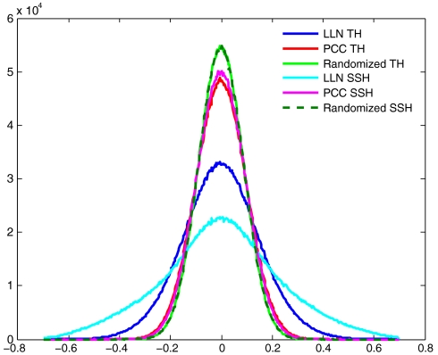
Correction of long-range correlations in probe ratios. A random set of 2,000 probes with nonredundant mappings to the reference genome (hg18 build) was selected. From these, two 2,000 X 132 matrices of log ratios were created: one for 132 SSH and another for 132 randomly selected TH. Pearson correlations between matrix rows were computed before LLN and after applying PCC. The histogram also shows the distribution of correlations for LLN matrixes with independent random permutation of values within rows. The bin size for the histogram is 0.003.

Not all trend patterns are alike, but appear composed of relatively independent components. One major trend is associated with GC content (8), but it is not the only one. We sought to correct for correlated system noise in those hybridizations plagued by it, while minimizing adjustment in hybridizations that are not. A simple tool for accomplishing just this utilizes principal component analysis (PCA). First, the major (low-dimensional) orthogonal basis for the system noise are found. Second, we maximize the fit of any given sample ratio data to these basis elements by least squares, and take the residual as the true genetic signal. To avoid mixing genetic signal with system noise in the principal components, we derive the components of system noise from self-self hybridizations (SSH), which contain no genetic signal. The results of such correction are illustrated (Author Summary, Fig. 1 D–F). This is what we call principal component correction (PCC).

We observe components of the noise that are readily detected by PCA but not corrected well by PCC. Therefore we tested one variant of our standard procedure. Rather than treat all hybridization probes equally from a mathematical perspective, we partitioned the probes into those sensitive to particular components of system noise and then separately used PCC to correct the probes within partitions. We call this “piecewise” principal component correction (PPCC).

The mathematical details, including how we choose the number of principal components for PCC, how we determine probe partitions for PPCC, and the special treatment of the sex chromosomes, are found in the Material and Methods.

System Correction Using Self-Self Data.

Ideally, there should be no long-range correlation between probe ratios for SSH data beyond what is expected from random process. But self-self ratio vectors do contain more long-range correlations than expected, reflecting the presence of correlated system noise. To view the extent of these correlations and their correction by our method, we used 2,000 probes chosen randomly, and then computed the pairwise Pearson correlations of these probe ratios across various datasets, before and after PCC. For comparison to randomized data, we also computed the distribution of correlations in data when the probe values were permuted within hybridizations (Materials and Methods). Upon correction we reduce the long-range correlations in SSH data, nearly to what is expected by random process. Histograms of the pairwise correlation values are shown (Fig. 1).

We next applied this method to sample-reference vectors, which we term “test hybridizations” (TH). By the Mendelian law of independent segregation, there should again be no long-range correlation in test data beyond what is expected from random process. After PCC, TH also had reduced long-range correlations (Fig. 1).

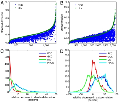
To assess PCC further, we measured two types of noise in the autosomal probes of TH before [local and Lowess normalization (LLN)] and after (PCC) correction: the standard deviation (Fig. 2 A, C), and the autocorrelation, which is the Pearson correlation of the ratio vector with itself shifted by one index (Fig. 2 B, D). The first measures overall noise, and the second measures local trends in the data. High autocorrelation would likely result in false segmentation, whereas high overall noise would lead to false negative segmentation. True genetic signal in the form of copy number variation would contribute to both measures, so to compute these measures we used a subset of the autosomal probes that are not commonly polymorphic (with a frequency of < 1%) in the best set of hybridizations, the “quiet autosomal probes.”

Fig. 2.

Comparison of PCC to other normalization schemes. (A) The standard deviation of log ratios for “quiet autosomal probes” of 1,349 female hybridization were scaled by the mean values of stable X chromosome regions before (green) and after (blue) noise correction, sorted by increasing standard deviation before PCC. (B) Autocorrelation was calculated for the log ratios of these probes from 3,252 hybridizations before (green) and after (blue) PCC, again sorted by increasing autocorrelation before correction. (C) Histograms for relative percent decrease of standard deviation for four different noise corrections: PCC, GCC, MS, or PPCC. The bin size is 1% decrease. (D) Histograms for relative percent gain/loss of autocorrelation of “quiet probes” for four different noise corrections: PCC, GCC, MS, and PPCC. (PPCC refers to piecewise principal component correction; MS and PPCC are described in detail in the Materials and Methods.) In this panel, the bin size is 3%. Quiet probes are defined as autosomal probes for which the frequency of amplifications and deletions combined does not exceed 1% within the population. Amplifications and deletions are defined here as segments exceeding ± log(1.1). Relative percent gain/loss for quantity X is defined as (100^∗(X_before - X_after)/X_before)%, where X_before is the value after Lowess and local normalization (LLN).

When the reference is male, the median of the ratio on the X chromosome in a female sample (excluding the pseudoautosomal regions) is an obvious measure of signal strength. We scale the standard deviation by this median X ratio. This adjustment is not readily available for males, so the results shown in Fig. 2 A and C are from females only. For comparison, we used the measures of noise in data subject only to LLN (Materials and Methods). We also assessed two other methods, based on the mean value of each probe ratio over the SSH dataset: mean subtraction (MS, Materials and Methods), and GC bin correction (GCC) for each hybridization (18). When PCC was applied, 100% of test hybridizations had decreased total noise and 91.51% had decreased autocorrelation. The mean relative improvement (100^∗(before - after)/before) of total noise is 11.2%, and the mean relative improvement of the autocorrelation is 33.1%. Compared to PCC, MS and GCC appear to decrease system noise and autocorrelation only marginally (Fig. 2 C, D).

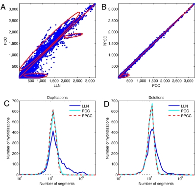
The impact of PCC on segmentation—a common method for determining regions of copy number variation—is found by examining the frequency with which certain regions of the genome are segmented. In SSH data, the numbers of segments—which by experimental design are false positives—were reduced more than 30-fold, from an average of 112 per hybridization to an average of 3 (Table S1). To monitor this sensitively in test data, we counted events exceeding a low-amplitude threshold (Fig. 3A) before and after correction. For each autosomal probe on the array, we counted how often it was observed contributing to a segment with a median ratio above a threshold of natural log(1.1). We plotted segmentation counts at each probe from the set of 3,252 test hybridizations as before (LLN, X-axis) vs. after (PCC, Y-axis) correction. The frequency of a large set of segments detected before system correction was drastically reduced after PCC (Fig. 3A, region “A”). We expect that these segments are false positives arising from genomically clustered system noise. We have direct confirmation of this by other methods (discussed later). The frequency of a few common copy number polymorphisms decreased modestly upon PCC (Fig. 3A, region B), and the probes from these regions often overlap with regions in our reference genome where the reference genome has copy number zero. We did not see entirely new regions of segmentation that became common only after PCC, as would likely be the case if false positives were being introduced. On the other hand, the frequency of detection of many common events actually increased upon PCC, which we think happens as a result of improved signal-to-noise in some of the noisier hybridizations (Fig. 3A, region C). The distribution of number of segments, both deleted and duplicated, in all hybridizations is more “Gaussian” following PCC and PPCC (Fig. 3 C, D).

Fig. 3.

Comparison of normalization methods in sample-reference hybridizations. Data for probes on all autosomes, before and after PCC or PPCC, were segmented from 3,252 hybridizations, median segmented ratio values assigned to each probe, and values above a 1.1 ratio threshold were counted. (A) Amplification count, with LLN (X axis) vs. PCC (Y axis). Circled region A represents a large set of segments detected before PCC, which are mostly not detected as segments after PCC; circled region B indicates a subset of very common copy number polymorphisms that are detected somewhat less frequently following PCC. Circled region C shows the common copy number polymorphisms that are detected more frequently following PCC. (B) Same as (A), except PCC (X axis) is compared to PPCC (Y axis). The circled region represents a small set of probes that are less frequently segmented for which the correction is improved. (C, D) Histograms of the number of segments with mean ratio value exceeding 1.1 (duplications) and less than 1/1.1 in ratio mean value (deletions). Bin size for number of segments is fixed in logarithmic scale.

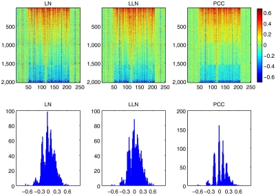
Another way to gauge the effectiveness of system correction is by examining the clarity of underlying copy number states. For any region of copy number polymorphism, variation should be observed as discrete states within the human population corresponding to integer increments of copy numbers. For most simple polymorphic regions (few states), the quantal nature of states is apparent before correction. However, for more complex situations (many states), multiple distinct states were readily observed only after PCC. An example of one such region, chosen from a subset of CNPs of > 10% frequency in the sampled population, is shown (Fig. 4). Without PCC, four peaks representing distinct copy number states are apparent (lower panels “LN” and “LLN”). After PCC, at least six discrete copy number states could be cleanly distinguished (lower right panel “PCC”).

Fig. 4.

Discrete copy number states at a commonly polymorphic site after PCC. The selected region (chr7:143504894-143707170, hg18 build) consists of a CNV locus (encompassing 170 probes) with 40 nonpolymorphic flanking probes on each side (X axis). Upper: the log ratio values of 2,028 hybridizations (Y axis) for all probes in the extended region are shown, for which rows are sorted in descending order by segment median ratios within the CNV. Lower: histograms of segment median ratios corresponding to the panels directly above. Following local normalization (Left) and LLN (Middle), varying copy number states are only moderately evident. PCC (Right) resolves at least six distinct states at this locus.

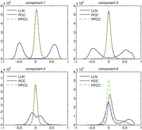
Finally, we can judge the extent of completeness of correction. We initially examined correlations of a set of randomly chosen 2,000 probes (Fig. 1). The correlations in these probes appeared very completely corrected. However, we found that certain probes were more affected by specific components of system noise than other probes, and the mere detection of a system noise component does not mean these components can be corrected by PCC. To explore this, we computed the Pearson correlations of the ratios of these “extreme” probes (i.e., those with the highest and lowest 0.1% of loadings for each PC) over the entire set of parents. We intentionally excluded data from offspring from these calculations to eliminate correlated (inherited) genetic signal. We made histograms of correlations, before and after PCC (Fig. S1). Correlations in the ratios for the extreme probes of all but the ninth PC were corrected following PCC, with extensive correction for the first, third, fourth, and fifth components. The ratios of the extreme probes of the ninth component were unusual in that they showed very high correlation, which was not strongly reduced upon PCC (Fig. 5). This is a matter of concern, because the probes of extreme loadings in the ninth PC are clustered in genome order, as we present in the next section.

Fig. 5.

Extent of probe correction following PCC and PPCC. For each of 14 components, a matrix of log ratios was created, consisting of 1,500 columns, one for each hybridizations of the parents, with about 4,200 rows, and one for each probe with extreme loadings (most positive and negative 0.1% of values). Pearson correlations were computed between all pairs of rows. Histograms of these correlations are shown for components 1, 3, 5, and 9, before and after PCC or PPCC. (Fig. S1 shows histograms for all principal components.) The bin size for the histograms is 0.005.

Association of the Principal Components with Probe Properties.

Examining the properties of the principal components, in particular their associations with known operational and system variables, reveals the richness and structure of system noise within the NimbleGen HD2 2.1 million probe platform.

We examined the association of the extreme probes in each PC with four probe properties: the location of probes on the microarray surface; the nucleotide composition of the probes; the clustering of the probe coordinates in the genome; and the position of the probes in relation to known functional units of the genome. Extreme probes from the fifth through eighth and from the tenth through fourteenth PC exhibit spatial clustering on the array surface (Fig. S2). The extreme probes from the first, second, and fifth PCs have especially significant compositional bias compared to random sets of probes (Table S2). For the first and fifth components, the base composition of probes with extreme positive loadings is strongly enriched for C + G and depleted for A + T, and the reverse is true for the probes with extreme negative loadings. For the second component, probes with extreme high loadings are depleted in A and enriched for T relative to the probes with extreme low loadings, with C and G being unaffected.

Extreme probes from the first, third, fourth, and ninth components showed clustering in the genome. This is reflected in the strong autocorrelation of the PCs themselves, with the first (0.35) and ninth (0.33) autocorrelations the strongest, compared to the autocorrelation of other components such as the second (0.05, Table S3). Clustering leads to spurious segmentation. Hence, these four components are of greatest interest to us, as they can be responsible for false positive segmentation. As is well known, the C + G base composition is not randomly distributed in the genome (19–21). The autocorrelation of the first component almost certainly reflects the C + G bias of the genome (Fig. 6A).

Fig. 6.

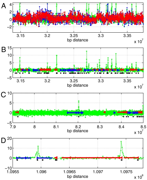
Loadings from components 1 and 9 in genome order, in relation to G + C nucleotide content and gene transcription units. (A) We examined the scaled (by 10³) loadings of components 1 (red) and 9 (green) in genome order from a representative gene-rich region. The blue is the C + G content of each probe (shifted and scaled), showing the rough overlap of the loadings of component 1 and the C + G content of the probes. (B) The coincidence of peaks of loadings in component 9 is illustrated with respect to genes in the same region. Green lines indicate loadings of component 9; blue and red represent forward- and reverse-strand genes, respectively; and the arrows indicate the direction of transcription and gene boundaries. Black asterisks show the genomic positions of CpG islands. (C, D) The same relationships shown in (B) are displayed in different regions and at different scales. Probes with high loading from the ninth component are clustered about the 5′ ends of genes, especially genes with nearby CpG islands. All information is derived from the hg18 build and UCSC Genome Browser (http://genome.ucsc.edu/) with coordinates on chromosome 1 as indicated on the X-axis.

The autocorrelation for the ninth component was of greatest interest to us because the autocorrelation was strong, and the ratios of the extreme probes were not corrected well by PCC (Fig. 5). This component does not have an exceptional compositional bias. It does not follow the C + G composition of the genome (Fig. 6A). Unlike the other components, the distribution of the loadings has a long one-sided tail (Table S3). The probes from this tail have a distinctive distribution in the genome (Fig. 6 B–D); they tend to cluster near those transcriptional start sites of genes that also contain CpG islands (22). We define a probe cluster as a maximally contiguous set of at least three probes within the top 1.5% of loading values, and we define the probe-cluster interval as that spanning the first and last probes. With these definitions, there were 3,415 cluster intervals for the extreme 1.5% probes of component nine: 57% overlap the 5′ end of a gene; 68% overlap CpG islands; and 54% overlap both. Such a level of overlap is highly unexpected based on simulations: we randomly created 3,415 new probe-clusters from our probe set and recomputed the percentage of overlap with the 5′ ends of genes. In 100 simulations, the overlap ranged from 5 to 7%. The observed overlap, 57%, lies so far outside this range that its p-value is far below that inferred by simulation (10^-2). Extreme probes of the other components did not form many probe clusters associated with the 5′ ends of genes (Table S4).

Association of Operational Variables with Principal Components.

The production of hybridization data depends upon several operational variables: the cell source; preparation and transport of samples; the synthesis of microarrays; the hybridization and wash conditions; and the settings and conditions of microarray scanning. A single variable, the “sample queue index,” captures much of this information in the order of processing and the placement of samples within microwell plates. For samples delivered in 96 (8-by-12) well plates, we define the queue index as the sum of the plate (or batch) number in order received, processed and shipped, (from 0 to 40) times 96, plus the row number (from 0 to 7) times 8, plus the column number (from 1 to 12) for each sample.

To measure the strength of the association of each component with each test ratio vector, we computed the Pearson correlations on a subset of extreme probes before (LLN) and after PCC, and plotted these correlations as a function of the queue index for all fourteen components (Fig. S3). The influence of each component is a rough function of the batch, and corrected by PCC—for all but the ninth component.

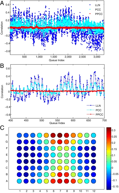
The correlation of the ninth component shows an unusual pattern. Its strength has a periodicity of 12 with respect to the queue index (Fig. 7 A, B). A periodicity of 8 emerges when the index is computed by plate row rather than column. To see the dependence on placement of samples in the 8-by-12 microwell format most clearly, the correlations in each sample plate were normalized to a mean of zero and standard deviation of one, and then the normalized correlations from microwells with identical row and column numbers were averaged. This computation is presented as a heat map in which each well value is represented as a disc in its proper plate position (Fig. 7C). It is clear that the ninth component captures variability in these hybridizations that are a function of well coordinates, in which the distance from the long and short edges of the plate are the critical variables. No other noise component displays this pattern.

Fig. 7.

Correlation of component 9 with microwell sample coordinates. Variation in correlation of component 9 with extreme (1.5% most positive and negative) probes over 3252 hybridizations has a periodicity of 12 with respect to the queue index (A and B), before (LLN) and after PCC, but not after PPCC. For (C), correlations computed for LLN data were adjusted in each 96-well plate to have a mean of zero and a standard deviation of 1. The adjusted values were then averaged over the same row and column coordinates from the 41 8-by-12 microwell plates in which the samples used for the hybridizations were stored and shipped. These values are displayed in microwell coordinates, with red for highly positive and blue for highly negative correlations.

Piecewise Correction for the Ninth Component.

PCC leaves much of the correlation between the log ratios of the extreme probes of the ninth component uncorrected (Fig. 5). The ninth component strongly affects a sufficient number of probes to be detectable as a principal component, but an insufficient number in any given ratio vector to force correction against the contravening introduction of white noise caused by the correction. Because these probes are clustered in the genome, they can (and do) give rise to spurious segmentation that remains uncorrected. As an example, we found several recurrent segments in LLN data from chronic lymphocytic leukemia (CLL) that were all highly correlated in leukemias (Fig. S4). The probes from these regions are among the extreme probes of component nine. Evaluating the genomes on other platforms (tiling microarrays from Agilent) and by PCR and DNA sequence analysis did not confirm the segmentation results. PCC failed to correct the data.

To address this we tested a nonlinear treatment of the data. We ranked all probes by their loadings in the ninth component and grouped probes in batches of 50,000 by their rank, thus partitioning the 2.1 million probe set. The probes with high loadings in the ninth component are thus heavily represented in one batch of probes. We applied PCC to each batch of probes separately (Materials and Methods). Corrected batches were assembled piecewise to form the whole genome. We call this method piecewise principal component correction (PPCC). The results of PPCC were similar to PCC (Fig. 2 C, D; Fig. 3B), and the extreme probes from the ninth component were better corrected (Fig. 5 and Fig. 7A). But the correlations between the probes still persist. Possible reasons for this are discussed below.

Discussion

We have been engaged in genetic studies of children affected with disorders (autism, congenital heart disease, and pediatric cancer) born to otherwise healthy parents. We search these children for genomic copy number variants not seen in either parent because new variation seen in the child provides strong clues to the genetic origins of the disorders (17, 23–25). Such de novo events are truly rare, so it has been critical for us to minimize false positive discovery rates. CGH often contains probe-clustered and correlated noise, or trends, that produce false positives through spurious segmentation, so we have been highly motivated to correct for these artifacts. We report here a method for correcting genome copy number data by taking the residuals to the linear combinations of the principal components of the noise that best fit the data.

Computing residuals to the principal components derived from the test data is problematic, because those principal components also contain genetic signal, namely the copy number differences between the genomes of the subject and reference genome. Thus, using test data corrupts the corrections. To solve this, we hypothesized that major system noise is also present in self-self hybridizations. In self-self hybridizations, we expect no genetic signal, and any analysis of variability should reflect only system noise. We designed our data collection with self-self hybridizations liberally inserted into the production pipeline. Much of the system noise that afflicts sample-reference hybridizations is also found in the self-self hybridizations, and therefore we could use the latter to correct for noise in the former. We chose principal component analysis rather than factor analysis because the former does not require any a priori probabilistic model, whereas factor analysis does. Statistical methods other than principal component analysis could certainly be employed to achieve and possibly improve correction, and we expect to explore this avenue in future work.

As strong validation of our approach, the properties of the major principal components reflect known system and operational variables. For example, the extreme probes in several components reflect the layout of probes on the array, consistent with the expectation that some variation arises from fabrication and/or physical processing of the arrays. Also, extreme probes from the first two components have striking biases in their base compositions. The extreme probes of the first component are biased by C + G content. This was expected, given the strong influence of C + G density on autocorrelation observed in earlier CGH experiments on a number of platforms (26, 27). Because the efficiency of hybridization varies with C + G content of the probes, the first component may reflect imprecisely controlled hybridization and washing conditions. This component is also responsible for major trends in the data, as expected from the presence of C + G rich isochores distributed throughout the genome (19, 20, 28). The probes of the second component have a bias in A at one extreme and in T at the other. The second component is the most invariant of all the components with respect to the operational variable of time, and hence it may arise from a physiochemical interaction of the nucleotides with the fluorophores.

Overall metrics of noise, especially autocorrelation, improve with our method. Nevertheless, correction is not complete. There are still hybridizations that show excess segmentation, and hybridizations that are outright failures. More troubling, however, is the noise from the unique ninth component. This component has a unique segmentation signature: the segments are narrow, and probes with extreme loadings often map to intervals containing both the 5′ ends of genes and associated CpG islands. These probes are not themselves especially rich in C + G. Perhaps a feature of the chromatin structure surrounding certain regions leaves a footprint when DNA is prepared or handled. Indeed, the magnitude of the association of the ninth component is dependent on the coordinates of the sample in its 96-well plate. Although the samples are not initially prepared in 96-well order, they are shipped and subsequently processed retaining that order. Thus this variation may reflect either freezing and thawing, or drying, as these physical parameters relate to the footprint from chromatin structure.

Hybridizations can have reasonably low noise, yet still have distorted ratios in certain chromosomal regions leading to spurious segmentation-even after PCC. Until we realized this, we were puzzled by a set of apparent small copy number events in leukemias that we could not validate using other methods of copy number measurement such as quantitative PCR and tiling microarrays. Eventually, we realized that these segments were all derived from the extreme probes of the ninth component. We can improve the correction of these probes by partitioning probes according to their loadings in the ninth component, performing principal component correction on each partition separately, then reassembling the whole genome piecewise (PPCC). By concentrating probes that are noisy with respect to one component, we can correct them better for that component.

Still, the correction for component 9 is not totally satisfactory. That may be in part because there is a variable biological factor at play, such as chromatin structure leaving an imprint on the DNA extracted from samples. This problem could become even more vexing if samples (and the reference) are drawn from different tissue sources. Nevertheless, our experience with the use of self-self hybridizations on the HD2 platform led us to ascertain certain genomic characteristics associated with false positives. As mentioned earlier, most artifacts of the ninth component have a unique signature. Based on this, a manual curation of the families from the SSC (17) significantly reduced the false positive rate (judged by orthogonal validation on tiling arrays) relative to other studies of similar scope (24, 29). It is worth noting that we do not see ninth component-like artifacts on data from the Illumina IMv1 and IMv3 Duo microarray platforms, which utilize a very different labeling and hybridization scheme. This component may be specific to our protocol. Nevertheless, it is likely that applying PCC to self-self data from other platforms and protocols would reveal novel artifacts that arise from differences in the underlying technologies.

The method for correcting copy number data that we propose adds some additional expense to experiments, but the cost of adding a few self-self hybridizations is minimal—less than 5% of the total number of hybridizations. Moreover, our results are comparable or better than the common expedient of adding duplicate color-reversed hybridizations (30), which essentially doubles the cost of a study. Work in progress indicates that the method of projecting to principal components can be used to suppress noise even when data derives from a single channel, using repetitions of a single reference to derive the components of the system noise. This can halve again the cost of assay. We expect that reducing system noise by adjusting for the principal components of that noise should be generally applicable to copy number data gathered from any platform, including DNA sequencing. In preliminary work, we observe long-range correlations with multiple independent components in copy number measurements from other platforms, which we intend to explore fully in future work.

Materials and Methods

Origin of Test and Self-Self Ratio Vectors.

Our dataset consists of a group of 3,252 test (sample-reference) hybridizations and a group of 132 self-self hybridizations. The latter group was comprised of 83 self-self hybridizations of our standard human male reference genome and 49 self-self hybridizations of other sample genomes, chosen at random. All test hybridizations were performed with the same male reference DNA and the same choice of dye labels: Cy3 for the sample and Cy5 for the reference. The self-self group consists of hybridizations with various batches of reference DNA or sample in both channels. The self-self hybridizations were randomly interspersed among a larger set of CGH experiments performed over a period of approximately 1 y. Blood samples were collected at a variety of centers throughout the United States. Sample and reference DNAs were prepared either from whole blood or from EBV-immortalized B-cells at the Rutgers University Cell and DNA Repository (RUCDR). DNAs were prepared robotically, then distributed and stored in 96-well plates. We track the reference batch number and the sample queue indices (microwell plate, column and row). All hybridizations were performed by NimbleGen in their Icelandic facility. DNAs were labeled by random priming incorporating a fluorescent cytosine nucleotide derivative. The platform was a NimbleGen HD2 CGH microarray with 2.1 million probes, the positions of which were randomized across the array surface. Composition and locations of probes on the array were kept fixed throughout the period of data collection.

We do not perform background subtraction. Rather, we employ other steps in data processing that are commonly used in the field, namely local and Lowess normalization (LLN) of probe intensities (14, 31).We will refer to the natural logarithm of ratios of such normalized probe intensities—when placed in genome order—as LLN “ratio vectors.” When we remove the data from the X and Y chromosomes, we refer to the remaining data as autosomal ratio vectors.

We segment ratio vectors into distinct regions of constant copy number by minimizing variation and using Kolmogorov-Smirnov (KS) statistics to determine if the segmentation passes the threshold of significance (32). The observations we discuss are essentially unchanged if we use other segmentation procedures such as circular binary segmentation (11).

System Correction with the Self-Self Archive.

We view the ratio data as a point in a 2.1-million dimension vector space. The basic idea is to derive the PCs from self-self data, and then correct the test data by subtracting from each its orthogonal projection to the hyperplane determined by the PCs. More specific details are as follows.

The matrix represents the local and Lowess normalized log ratios. Pseudo code for the local and Lowess normalization is presented in the Supplemental Information. Probe index i ranges from 1 to N (N = 2,161,679) and hybridization index k ranges from 1 to M + L, where M = 3,252 is the number of test hybridizations and L = 132 is the number of self-self hybridizations. In vector form we can write

[1]

where G^k, S^k, and ε^k are unobserved vectors in the N dimensional linear vector space W. G^k is the genetic signal vector representing copy number differences between the sample and the reference, a piecewise constant function of the probe index i for each hybridization k. S^k is the major system noise vector; and ε^k is residual noise. To determine S^k we use singular value decomposition in self-self hybridizations, where G^k is zero. For these hybridizations the singular value decomposition of the N by L submatrix A, composed from columns Y^k,k = M + 1,…,M + L is

[2]

where U is an N by L matrix with orthonormal columns, D is an L by L diagonal matrix with nonnegative singular values on the diagonal; and V is an L by L matrix with orthonormal columns, and V^T is its transpose. Singular values decrease sharply, which indicates that most of the variation in self-self hybridizations is concentrated in a lower dimensional subspace spanned by the first few columns U^′ (major principal components) of matrix U. To avoid verbosity, we will use notation U^′ for both the submatrix of U and the space spanned by its columns. To correct Y^k for system noise, we subtract from Y^k its orthogonal projection to this subspace. Algebraically this is presented by equation

[3]

We next posit that the components of system noise captured by the self-self hybridizations (and described by the principal components) are also shared in test hybridizations, and correct system variability in the latter by subtracting from them their projection onto the subspace U^′. As a practical matter, to compute the coefficients of the orthogonal projection to U^′ in terms of the principal components, we use only the probes from the autosomal region of the genome in part U^′TY^k of Eq. 3. This circumvents the distortion in the projection that would be caused by large areas of the genome with known differences in copy number between the sample and the reference when the sample is from a female (the unavoidable consequence of using a male reference genome).

To determine the number of major principal components—those with the largest singular values—we compared the singular values from self-self ratio vectors to vectors formed from them by within-row-permutation of the N by L matrix A of self-self vectors, where N is the number of probes and L is the number of SSHs. This permutation obliterates the correlations between probe ratios arising from system noise but maintains the mean and standard deviation for each probe ratio within the SSH archive. The comparison suggested taking the first 14 principal components defining submatrix of matrix (see “singular values” in Table S1 and Fig. S5). Another method, the Scree plot, suggested using the same number of major principal components (33).

Mean Subtraction (MS).

After all SSH are normalized (removed mean and divided by standard deviation), we compute vector X of log ratio averages across SSH. MS correction is taking the residual after projecting Y^k to X. Formally,

[4]

Piecewise Principal Component Correction (PPCC).

PCC leaves much of the correlation between the log ratios of the extreme probes of the ninth component uncorrected (Fig. 5). To address this, we explored a nonlinear version of our method. We took a two-stage approach. First, we computed PC as indicated in the previous section. Then we ranked all probes by their loadings in the ninth component and grouped probes in batches of 100,000 by their rank, thus partitioning the 2.1 million probe set. The probes with high loadings in the ninth component are thus heavily represented in one batch of probes. We applied PCC (Eq. 3) to each batch of probes separately, with their autosomal part equal to the intersection with autosome probes of the whole genome and their X and Y part equal to the intersection with probes on X and Y chromosomes. Corrected batches are assembled piecewise to form the whole genome. We call this method piecewise principal component correction (PPCC). MATLAB code for both PCC and PPCC is included in the Supplemental Materials.

References

- 1.Iafrate AJ, et al. Detection of large-scale variation in the human genome. Nat Genet. 2004;36:949–951. doi: 10.1038/ng1416. [DOI] [PubMed] [Google Scholar]
- 2.Sebat J, et al. Large-scale copy number polymorphism in the human genome. Science. 2004;305:525–528. doi: 10.1126/science.1098918. [DOI] [PubMed] [Google Scholar]
- 3.Nei M, Niimura Y, Nozawa M. The evolution of animal chemosensory receptor gene repertoires: Roles of chance and necessity. Nat Rev Genet. 2008;9:951–963. doi: 10.1038/nrg2480. [DOI] [PubMed] [Google Scholar]
- 4.Perry GH, et al. Diet and the evolution of human amylase gene copy number variation. Nat Genet. 2007;39:1256–1260. doi: 10.1038/ng2123. [DOI] [PMC free article] [PubMed] [Google Scholar]
- 5.Stankiewicz P, Lupski JR. Structural variation in the human genome and its role in disease. Annu Rev Med. 2010;61:437–455. doi: 10.1146/annurev-med-100708-204735. [DOI] [PubMed] [Google Scholar]
- 6.Zhang F, Gu W, Hurles ME, Lupski JR. Copy number variation in human health, disease, and evolution. Annu Rev Genomics Hum Genet. 2009;10:451–481. doi: 10.1146/annurev.genom.9.081307.164217. [DOI] [PMC free article] [PubMed] [Google Scholar]
- 7.Quackenbush J. Microarray data normalization and transformation. Nat Genet. 2002;32(Suppl):496–501. doi: 10.1038/ng1032. [DOI] [PubMed] [Google Scholar]
- 8.Marioni JC, et al. Breaking the waves: Improved detection of copy number variation from microarray-based comparative genomic hybridization. Genome Biol. 2007;8:R228. doi: 10.1186/gb-2007-8-10-r228. [DOI] [PMC free article] [PubMed] [Google Scholar]
- 9.Messer PW, Bundschuh R, Vingron M, Arndt PF. Effects of long-range correlations in DNA on sequence alignment score statistics. J Comput Biol. 2007;14:655–668. doi: 10.1089/cmb.2007.R008. [DOI] [PubMed] [Google Scholar]
- 10.Neuvial P, et al. Spatial normalization of array-CGH data. BMC Bioinformatics. 2006;7:264. doi: 10.1186/1471-2105-7-264. [DOI] [PMC free article] [PubMed] [Google Scholar]
- 11.Olshen AB, Venkatraman ES, Lucito R, Wigler M. Circular binary segmentation for the analysis of array-based DNA copy number data. Biostatistics. 2004;5:557–572. doi: 10.1093/biostatistics/kxh008. [DOI] [PubMed] [Google Scholar]
- 12.Curtis C, et al. The pitfalls of platform comparison: DNA copy number array technologies assessed. BMC Genomics. 2009;10:588. doi: 10.1186/1471-2164-10-588. [DOI] [PMC free article] [PubMed] [Google Scholar]
- 13.Fang H, et al. Hybridization as an alternative experiment design to dye swap for two-color microarrays. Omics. 2007;11(1):14–24. doi: 10.1089/omi.2006.0002. [DOI] [PubMed] [Google Scholar]
- 14.Khojasteh M, Lam WL, Ward RK, MacAulay C. A stepwise framework for the normalization of array CGH data. BMC Bioinformatics. 2005;6:274. doi: 10.1186/1471-2105-6-274. [DOI] [PMC free article] [PubMed] [Google Scholar]
- 15.Leek JT. Asymptotic Conditional Singular Value Decomposition for High-Dimensional Genomic Data. Biometrics. 2010 doi: 10.1111/j.1541-0420.2010.01455.x. DOI: 10.1111/j.1541-0420.2010.01455.x. [DOI] [PMC free article] [PubMed] [Google Scholar]
- 16.Leek JT, et al. Tackling the widespread and critical impact of batch effects in high-throughput data. Nat Rev Genet. 2010;11:733–739. doi: 10.1038/nrg2825. [DOI] [PMC free article] [PubMed] [Google Scholar]
- 17.Levy D, et al. Rare de novo and transmitted copy-number variation in autistic spectrum disorders. Neuron. 2011;70:886–897. doi: 10.1016/j.neuron.2011.05.015. [DOI] [PubMed] [Google Scholar]
- 18.Yoon S, Xuan Z, Makarov V, Ye K, Sebat J. Sensitive and accurate detection of copy number variants using read depth of coverage. Genome Res. 2009;19:1586–1592. doi: 10.1101/gr.092981.109. [DOI] [PMC free article] [PubMed] [Google Scholar]
- 19.Bernardi G. The human genome: organization and evolutionary history. Annu Rev Genet. 1995;29:445–476. doi: 10.1146/annurev.ge.29.120195.002305. [DOI] [PubMed] [Google Scholar]
- 20.Bernardi G, et al. The mosaic genome of warm-blooded vertebrates. Science. 1985;228:953–958. doi: 10.1126/science.4001930. [DOI] [PubMed] [Google Scholar]
- 21.Lander ES, et al. Initial sequencing and analysis of the human genome. Nature. 2001;409:860–921. doi: 10.1038/35057062. [DOI] [PubMed] [Google Scholar]
- 22.Illingworth RS, Bird AP. CpG islands—‘a rough guide’. FEBS Lett. 2009;583:1713–1720. doi: 10.1016/j.febslet.2009.04.012. [DOI] [PubMed] [Google Scholar]
- 23.Marshall CR, et al. Structural variation of chromosomes in autism spectrum disorder. Am J Hum Genet. 2008;82:477–488. doi: 10.1016/j.ajhg.2007.12.009. [DOI] [PMC free article] [PubMed] [Google Scholar]
- 24.Pinto D, et al. Functional impact of global rare copy number variation in autism spectrum disorders. Nature. 2010;466:368–372. doi: 10.1038/nature09146. [DOI] [PMC free article] [PubMed] [Google Scholar]
- 25.Sebat J, et al. Strong association of de novo copy number mutations with autism. Science. 2007;316:445–449. doi: 10.1126/science.1138659. [DOI] [PMC free article] [PubMed] [Google Scholar]
- 26.Cardoso J, et al. Genomic profiling by DNA amplification of laser capture microdissected tissues and array CGH. Nucleic Acids Res. 2004;32:e146. doi: 10.1093/nar/gnh142. [DOI] [PMC free article] [PubMed] [Google Scholar]
- 27.Lepretre F, et al. Waved aCGH: To smooth or not to smooth. Nucleic Acids Res. 2010;38:e94. doi: 10.1093/nar/gkp1215. [DOI] [PMC free article] [PubMed] [Google Scholar]
- 28.Duret L, Galtier N. Biased gene conversion and the evolution of mammalian genomic landscapes. Annu Rev Genomics Hum Genet. 2009;10:285–311. doi: 10.1146/annurev-genom-082908-150001. [DOI] [PubMed] [Google Scholar]
- 29.Sanders SJ, et al. Multiple recurrent de novo CNVs, including duplications of the 7q11.23 Williams syndrome region, are strongly associated with autism. Neuron. 2011;70:863–885. doi: 10.1016/j.neuron.2011.05.002. [DOI] [PMC free article] [PubMed] [Google Scholar]
- 30.Churchill GA. Fundamentals of experimental design for cDNA microarrays. Nat Genet. 2002;32(Suppl):490–495. doi: 10.1038/ng1031. [DOI] [PubMed] [Google Scholar]
- 31.Cleveland WS. Robust locally weighted regression and smoothing scatterplots. J Amer Statist Assoc. 1979;74:829–836. [Google Scholar]
- 32.Grubor V, et al. Novel genomic alterations and clonal evolution in chronic lymphocytic leukemia revealed by representational oligonucleotide microarray analysis (ROMA) Blood. 2009;113:1294–1303. doi: 10.1182/blood-2008-05-158865. [DOI] [PubMed] [Google Scholar]
- 33.Jolliffe IT. Principal Component Analysis. 2nd Ed. New York: Springer-Verlag, Inc; 2002. [Google Scholar]