Hybrid modeling and simulation of stochastic effects on progression through the eukaryotic cell cycle

Abstract

The eukaryotic cell cycle is regulated by a complicated chemical reaction network. Although many deterministic models have been proposed, stochastic models are desired to capture noise in the cell resulting from low numbers of critical species. However, converting a deterministic model into one that accurately captures stochastic effects can result in a complex model that is hard to build and expensive to simulate. In this paper, we first apply a hybrid (mixed deterministic and stochastic) simulation method to such a stochastic model. With proper partitioning of reactions between deterministic and stochastic simulation methods, the hybrid method generates the same primary characteristics and the same level of noise as Gillespie's stochastic simulation algorithm, but with better efficiency. By studying the results generated by various partitionings of reactions, we developed a new strategy for hybrid stochastic modeling of the cell cycle. The new approach is not limited to using mass-action rate laws. Numerical experiments demonstrate that our approach is consistent with characteristics of noisy cell cycle progression, and yields cell cycle statistics in accord with experimental observations.

INTRODUCTION

The eukaryotic cell cycle is regulated by a complicated chemical reaction network. To model the cell cycle control system, theoretical biologists previously used deterministic models based on ordinary differential equations (ODEs).^{1, 2, 3, 4, 5, 6, 7, 8, 9, 10} Although deterministic cell cycle models can be precise and robust in many respects, experimental data exhibit considerable variability from cell to cell during cell growth and division.^{11, 12, 13} For example, the coefficient of variation ($\mathrm{CV}=\frac{\mathrm{standard}\mathrm{deviation}}{\mathrm{mean}}$) of size at division for fission yeast cells is around 7.5%, and the CV of their cell cycle time is up to 14%.¹¹ This observed noise is usually attributed to two sources: intrinsic noise from fluctuations of molecule numbers present within a single cell; and extrinsic noise, from inequalities in sizes of the two daughter cells after division. Given the small volume of a cell (e.g., a yeast cell is roughly 30 fl at birth), the total number of molecules of a particular protein species is usually limited to several thousand. Moreover, the number of molecules of the mRNA for each protein at any time is normally less than 10.¹⁴ In this case, molecular fluctuations cannot be neglected, and they may significantly affect the behavior of the cell. Therefore, to accurately model the cell cycle, stochastic models and simulations are required to capture this noise.

A rigorous way to build a stochastic model is to convert a deterministic model into its stochastic equivalent, which employs only elementary reactions. The result is suitable for simulation by Gillespie's stochastic simulation algorithm (SSA).^{15, 16} One of the major difficulties in this type of conversion lies in the rate laws, which are often not elementary (mass-action) kinetics. For example, Tyson and Novak's simple three-variable model of the cell cycle⁷ (see Sec. 2) involves variables X, Y, and Z. The phosphorylation and dephosphorylation of Y are governed by Michaelis-Menten rate laws, and the synthesis of Z is given by a Hill function. These phenomenological rate laws are approximations, derived from more detailed elementary reaction mechanisms using pseudo-steady-state approximations. However, applying Gillespie's SSA to phenomenological rate laws may possibly generate incorrect stochastic results.¹⁷ Thus, a model based fully on mass-action kinetics for all reactions was developed in Kar et al.¹⁸ by “unpacking” the reactions with phenomenological rate laws in the Tyson-Novak three-variable model into sets of elementary stochastic reactions. In the process, mRNA variables for X, Y, Z, and other helper proteins were introduced into the network. The unpacked model was then simulated using Gillespie's SSA. The work of Kar et al. managed to model the repetitive cell cycle behavior on average and capture proper amounts of both the extrinsic and intrinsic noise. However, the cost is a much larger system of variables and reactions. If a more detailed deterministic model, such as Chen et al.,⁹ were to be unpacked for stochastic simulation, the complexity of the model would quickly increase as well as the central processing unit (CPU) time for simulation by Gillespie's SSA.

Our goal is to develop a modeling and simulation strategy for cell cycle models that is both accurate and efficient. First, to improve the simulation efficiency of Kar et al.'s stochastic model, we apply Haseltine and Rawling's hybrid method¹⁹ with different partitioning strategies, and check the corresponding accuracy and efficiency. We demonstrate that, with a more efficient partitioning strategy, the hybrid simulation gives reasonably accurate results and saves significant computational cost as compared to the full stochastic simulation. Furthermore, through an analysis of the partitioning results in the hybrid simulation, we conclude that a good partitioning strategy for a cell cycle model is to treat all reactions related to gene expression (reactions modifying gene and mRNA species) as “slow” reactions (meaning that they happen infrequently enough that they must be simulated stochastically). Biologically, it matches with our intuition that (for cell cycle models) most of the intrinsic noise arises at the gene expression level due to the low numbers of molecules of genes and mRNAs. On the other hand, it also implies that, to prepare a deterministic cell cycle model for stochastic simulations, one may not need to unpack the phenomenological rate laws. Instead, we managed to build a new hybrid model by packing Kar et al.'s model back to a comparable three-variable model. The ODEs are similar to the original three-variable model, while stochastic elementary reactions related to gene expression are added as slow reactions and simulated with the SSA. In this way, we avoid creating a large reaction network while obtaining sufficient accuracy and improved efficiency in simulation.

This paper is organized as follows. In Sec. 2, we provide a description of the cell cycle models that we base our work on. In Sec. 3, we briefly review Haseltine and Rawlings' hybrid method and then apply it to Kar et al.'s model. We discuss its accuracy and efficiency with different partitioning strategies. In Sec. 4, we propose a new hybrid stochastic cell cycle model, and we show evidence that the new model is able to correctly capture both the basic dynamics and the intrinsic noise of the cell cycle. In Sec. 5, we present an analysis for the new partitioning strategy. Our conclusions are summarized in Sec. 6.

CELL CYCLE MODELS

The cell cycle is driven by the mutual antagonism between B-type cyclins (such as Clb2) and G1-stabilizers (such as Cdh1).²⁰ When B-type cyclins are abundant, they combine with kinase subunits (Cdk1) to form active protein kinases (e.g., Cdk1-Clb5 and Cdk1-Clb2 in budding yeast) that promote DNA synthesis and mitosis (S, G2, and M phases of the cell cycle). When Cdh1 is active, Clb-levels are low, and cells are in the unreplicated phase (G1) of the DNA replication-division cycle. The cell cycle control system alternates back-and-forth between G1 phase (Cdh1 active, Clb-levels low) and the S-G2-M phase (Cdh1 inactive, Clb-levels high).

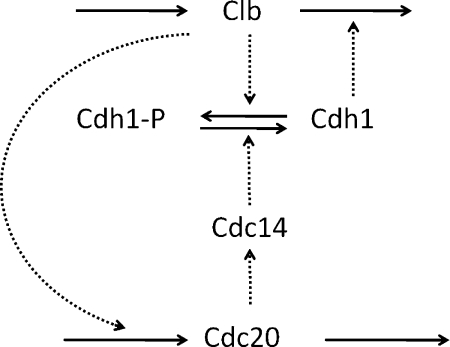
Tyson and Novak built their three-variable model⁷ based on a bistable switch created by the antagonism between Clb complexes, denoted by X in the three variable model, and Cdh1, denoted by Y, as illustrated in Figure 1.

Figure 1.

Bistable switch on which Tyson and Novak's model is based.

In this model, X inactivates Y by phosphorylating it, and the unphosphorylated Y catalyzes the degradation of X. The exit protein, Cdc20, activates a phosphatase (Cdc14) that dephosphorylates and activates Y. The actions of Cdc20 and Cdc14 are lumped together in a single variable Z, whose synthesis is promoted by X. Therefore, X is involved in a positive feedback loop with its repressor Y (mutual antagonism), which creates a bistable switch. Cell growth flips the switch from the G1 state to the S-G2-M state. The reverse transition (back to the G1 state) is triggered by the negative feedback loop in the model (X activates Z, Z activates Y, and Y inactivates X).

This three-variable model can be formulated as the following set of ODEs:⁷

$$\left\{\begin{array}{ccc}\frac{\mathrm{d}}{\mathrm{dt}}V\hfill & =\hfill & \mu V\hfill \\ \frac{\mathrm{d}}{\mathrm{dt}}\left[\mathrm{X}\right]\hfill & =\hfill & k_{\mathrm{sx}}V-(k_{\mathrm{dx}}+k_{\mathrm{dxy}}\left[\mathrm{Y}\right])\left[\mathrm{X}\right]\hfill \\ \frac{\mathrm{d}}{\mathrm{dt}}\left[\mathrm{Y}\right]\hfill & =\hfill & \frac{(k_{\mathrm{hy}}+k_{\mathrm{hyz}}\left[\mathrm{Z}\right])(\left[{\mathrm{Y}}_{\mathrm{T}}\right]-\left[\mathrm{Y}\right])}{J_{\mathrm{hy}}+\left[{\mathrm{Y}}_{\mathrm{T}}\right]-\left[\mathrm{Y}\right]}-\frac{k_{\mathrm{pyx}}\left[\mathrm{X}\right]\left[\mathrm{Y}\right]}{J_{\mathrm{pyx}}+\left[\mathrm{Y}\right]}\hfill \\ \frac{\mathrm{d}}{\mathrm{dt}}\left[\mathrm{Z}\right]\hfill & =\hfill & k_{\mathrm{sz}}+\frac{k_{\mathrm{smzx}}{\left[\mathrm{X}\right]}^n}{{J_{\mathrm{smzx}}}^n+{\left[\mathrm{X}\right]}^n}-k_{\mathrm{dz}}\left[\mathrm{Z}\right]\hfill \end{array}\right.,$$ (1)

where square brackets denote the concentration of a chemical species. The k's are reaction rate constants, and the J's are equilibrium binding constants (measured in terms of concentration). [Y_T] is the total concentration of Y (the sum of the phosphorylated and unphosphorylated forms). The Hill exponent, n, determines the steepness of the sigmoidal curve expressing the dependence of Z-synthesis on [X]. With proper choice of parameter values, this model shows alternations of G1 phase and the S-G2-M phase in deterministic simulations. A more detailed deterministic cell cycle model for budding yeast, developed by Chen et al.,⁹ successfully accounts for the phenotypes of wild-type budding yeast cells and about 120 mutant strains.

The equations in Eq. 1 represent a deterministic phenomenological model. In order to build a stochastic cell cycle model, the state variables have to be converted from concentrations (nM) to numbers of molecules per cell (“populations”), and new state variables have to be added to represent mRNA populations because intrinsic noise in cells is mostly generated at the gene expression level.^{21, 22, 23} Moreover, following Gillespie's framework of SSA, chemical reactions with mass action kinetics are desired to capture the full stochastic effect in chemical reaction systems. Thus, reactions that use phenomenological rate laws (such as Michaelis-Menten and Hill functions) must each be replaced by a series of reactions written with elementary mass-action kinetics using additional variables as intermediate species. The result is a much larger system of equations. Kar et al.¹⁸ built a stochastic cell cycle model with 19 variables and 47 reactions, based on Tyson and Novak's three-variable model. Kar et al.'s model generates distributions of cell cycle times and division sizes that match the data observed in wet-lab experiments. However, conversion from the original three-variable, phenomenological, deterministic model to the fully unpacked and supplemented stochastic model takes a great amount of work, and simulations of the unpacked model by Gillespie's SSA are slow. The goal of this paper is to reduce the modeling effort and to improve the efficiency of the stochastic simulation without sacrificing the accuracy of the model.

HYBRID METHOD AND PARTITIONING STRATEGIES

Hybrid method

For large systems with fast reactions, Gillespie's SSA can be computationally slow because it simulates every reaction event. “Fast” reactions are so called to contrast with “slow” reactions that occur comparatively infrequently. To speed up the SSA, several approximate simulation strategies have been proposed. One group of approximation methods tries to take advantage of the multiscale characteristics observed in the reactant populations. Some species are present at larger population numbers than others. If all reactants have relatively large populations, one can represent a stochastic system by chemical Langevin equations (CLEs) and solve them as stochastic differential equations,²⁴ or directly apply tau-leap methods,^{25, 26} which approximate the numbers of reactions by Poisson random numbers. The other group of approximation methods tries to take advantage of multiscale features in the reactions: fast reactions, by definition, occur much more frequently than slow ones. A quasi-steady-state assumption on the high-population variables²⁷ or a partial equilibrium assumption on the fast (high propensity) reactions²⁸ can be applied to reduce the system and accelerate the simulation. In realistically large biochemical systems, usually both multiscale features are present. Species populations and reaction propensities can each span several orders of magnitude. Thus, it is not realistic to simulate a multiscale system with only one method that works well in one scale. Instead, hybrid methods should be considered from a more practical, system-specific point of view.

Several hybrid methods have been presented.^{19, 29, 31} Cao et al.³¹ proposed to partition the system, based simply on the species population numbers. For species whose population numbers are less than a threshold, all related reactions are simulated by the SSA, while other reactions are simulated by the tau-leaping method. Haseltine and Rawlings¹⁹ proposed to partition a system into groups of slow and fast reactions. The partitioning criterion is determined by two thresholds set by the user before simulation. A reaction is put into the fast reaction group if its propensity is greater than the propensity threshold, and the populations of all its reactants are greater than the population threshold. In this method, the fast reaction group is governed by ODEs or CLEs and the slow reaction group is simulated by Gillespie's direct method. A similar strategy was adopted by Salis et al.,^{29, 30} but fast reactions are approximated by CLEs and slow reactions are simulated by Gibson and Bruck's next reaction method.³² They also developed a more efficient mechanism to monitor the occurrences of slow, discrete events while simultaneously simulating the dynamics of a continuous, stochastic or deterministic process.

Our work follows the original idea of the hybrid method from Haseltine and Rawlings,¹⁹ and adopts a similar implementation strategy for event handling as in Salis et al.^{29, 30} Suppose the system has N species, and its state vector is denoted by X(t) = (X₁(t), …, X_N(t)), where X_i(t) is the number of molecules of the ith species at time t. Suppose M reactions are involved. The M reactions are partitioned into two subsets: S_fast for fast reactions, which are formulated by ODEs, and S_slow for slow reactions, which are stochastic reactions. Let a_i(x, t) be the propensity of the ith reaction in S_slow when X(t) = x, τ be the jump interval of the next stochastic reaction, and μ be its reaction index. The ODE system is formed from the fast reaction set (S_fast) and the SSA system from the slow reaction set (S_slow). Set t = 0. The hybrid algorithm is given as follows.

Hybrid simulation algorithm

• 1.Generate two uniform random numbers r₁ and r₂ in U(0, 1).
• 2.
  Integrate the ODE system with the integral equation,

  $${\int }_t^{t+\tau }{a}_{\mathrm{tot}}(x,s)ds+\log \left(r_1\right)=0,$$ (2)

  where a_tot(x, t) is the total propensity of S_slow.
• 3.
  Determine μ as the smallest integer satisfying

  $$\sum _{i=1}^{\mu }{a}_i(x,t)>r_2{a}_{\mathrm{tot}}(x,t).$$ (3)
• 4.Update X(t) according to the μth reaction in S_slow.
• 5.If stopping condition is not reached, go to step 1.

Note that solving Eq. 2 is an important step, particularly when the slow reaction propensities change appreciably over time according to the fast reaction dynamics. The original strategy by Haseltine and Rawlings¹⁹ is to add a propensity of “no reaction” that decreases the time of the next slow reaction, τ, so that the slow reaction propensities do not appreciably change over time τ, while Salis et al.^{29, 30} introduced a system of jump differential equations, where each equation describes the propensity for a single slow reaction to occur. These jump equations are numerically integrated alongside the system of ODEs (or SDEs). When the solution to a jump equation crosses zero, its corresponding slow reaction has fired. This step is the key difference between the two algorithms. In our implementation, we follow a similar strategy as Salis et al. but apply it to the direct method instead of Gibson and Bruck's next reaction method.³² Suppose that the ODE system is given by

$$x^{\prime }=f\left(x\right).$$ (4)

We simply add an integration variable z and add an equation

$$z^{\prime }=a_{\mathrm{tot}}\left(x\right),z\left(0\right)=0.$$ (5)

At every simulation step, starting from time t, ODEs 4, 5 are numerically integrated until z(t + τ) = z(t) + log(r₁). Then, τ gives the solution for Eq. 2. This integration can be performed by a standard ODE solver with root-finding, such as LSODAR.³⁶

Partitioning strategy

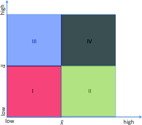
The hybrid simulation algorithm is straightforward, if the system is well partitioned. However, an important decision has to be made on the partitioning strategy. The original partitioning strategy proposed by Haseltine and Rawlings, which was adopted in the software package hy3S,^{29, 30} partitions the system with two thresholds pre-selected by the user. One is the population threshold $\overline{x}$, while the other is the propensity threshold $\overline{a}$. A reaction is considered as a fast reaction only when the populations of all its reactants are greater than $\overline{x}$ and its propensity is greater than $\overline{a}$. Figure 2 illustrates this strategy.

Figure 2.

Scales of reactions and populations. Region I contains slow reactions whose reactants have low populations; region II contains slow reactions whose reactants have high populations; region III contains fast reactions whose reactants have low populations; region IV contains fast reactions whose reactants have high populations.

Here, the scales are measured by the time average of the populations and propensities. The species populations and reactions are sorted from low to high. The whole system is thus divided into four regions, as illustrated in the figure. Haseltine and Rawlings' partitioning strategy puts regions I, II, and III into the SSA regime and region IV into the ODE regime. This is a conservative strategy. Unfortunately, simulations for both the ODE and SSA regimes have to stop and restart for every SSA firing. Thus, the efficiency of the hybrid method depends heavily on the stepsize allowed by the SSA, which is limited by the scales of the reactions in the SSA regime. Particularly, the reactions in region III, which contains fast reactions with at least one reactant/product with a low population, will force the system to take small steps. Thus, the efficiency of the hybrid method is limited by region III. This presents a challenge when the hybrid method is applied to model and simulate complex systems. In this paper, we propose a different partitioning strategy for the cell cycle model: We only put region I into the SSA regime, while reactions in regions II, III, and IV are all simulated with ODEs.

Applying the hybrid method to the cell cycle model

In preparing the Tyson-Novak three-variable model for stochastic simulation, Kar et al. not only converted the phenomenological rate laws (Michaelis-Menten and Hill kinetics) to elementary steps (mass-action kinetics) but also added stochastic reactions related to gene expression. We predict that most of the intrinsic noise in the cell cycle should come from the gene and mRNA species. These species have lower molecule numbers and react less frequently than protein level reactions. Meanwhile, the majority of the reactions are on the protein level, where insignificant noise is expected. These two levels suggest a natural partitioning of the system. But all these conjectures need verification from numerical results.

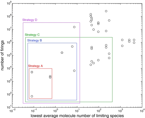
To find an appropriate partitioning of this system, we first generated a sample SSA run on the fully stochastic model to collect scale information for all the reactions from the simulation profile. Two characteristics are calculated and plotted in the sample run. One is the time average population for each species. The other is the total number of firings for each reaction. (In the SSA, the total number of firings, which is easy to track, is equivalent to the scale of the integral of the propensities.) Figure 3 shows (on a double-log plot) the profile for all 47 reactions in Kar et al.'s model in terms of these two characteristics. Each circle represents a reaction. Some circles may overlap due to the resolution of the image. Note that for each reaction, its population scale is determined by the smallest time average population of all its reactants and products, but not catalysts.

Figure 3.

Profile of reactions in Kar's cell cycle model. Data are collected from a sample SSA run for continuous 200 cell cycles. Four partitioning strategies A, B, C, and D are represented. For each of them, the reactions in the box are for the SSA system, while the ones outside the box are for the ODE system.

We test four partitioning strategies as illustrated in Figure 3. Starting from the lower left part of the profiling plot, we initially partition the five slowest reactions with the lowest molecule numbers into the SSA system (strategy A). These reactions fire less than 10 000 times in 200 cycles (the total number of reaction events is about 10⁹) and their reactants have average populations less than 1. Three of them control the activation/inactivation of the gene and two of them are synthesis and degradation of mRNA for protein Z. We predict that these reactions should be the main source of intrinsic noise. In strategy B, we add nine more reactions into the SSA system. These reactions fire less than 10⁶ times in 200 cycles, and their reactants have average populations less than 10. They are all on the gene expression level. Eight of them are mRNA synthesis and degradation reactions and one is related to degradation of the transcription factor. Strategies A and B both follow the idea of partitioning only region I into the SSA regime. The difference is only on the threshold values. Interestingly, in strategy B the SSA regime includes all the reactions related to gene expression. For comparison purposes, we also tried two more partitioning strategies. Strategy C includes ten more slow reactions (<10⁶) with high populations (>30), while strategy D includes two more fast reactions (>0⁶) with low populations (<10).

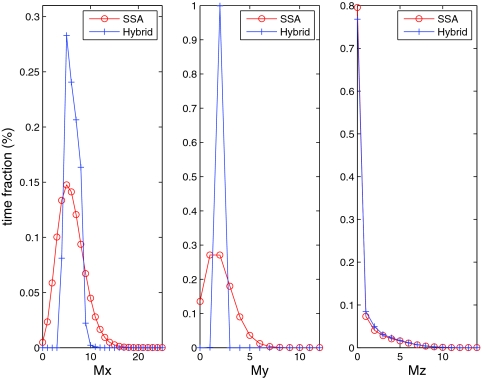
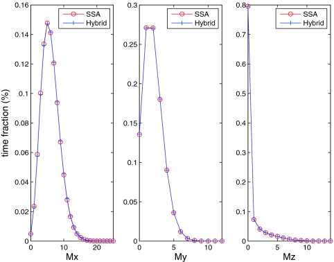
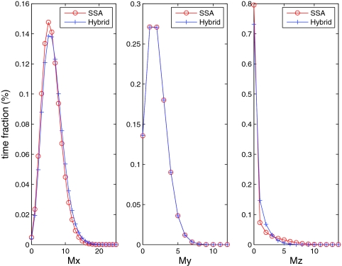
Since the mRNAs for proteins X, Y, and Z are crucial indicators of this cell cycle system, in order to analyze the impact of the four partitioning strategies we first compare the hybrid method to the SSA on these distributions. Figures 45 show the comparison for strategies A and B, respectively. For strategy B (Figure 5), both methods generate nearly identical distributions of the mRNAs because all reactions related to the mRNAs are treated stochastically. For strategy A (Figure 4), only the mRNA for Z (M_z) has matching distributions because the other two mRNA variables (M_x and M_y) are included in the ODE system. Therefore, we can see from Figure 4 that M_x and M_y exhibit much smaller variances than they do in the full stochastic simulation. We do not show comparisons for strategies C and D, because they give the same results as strategy B (Figure 5).

Figure 4.

mRNA distributions for the hybrid method and the SSA on Kar et al.'s cell cycle model. Partitioning strategy A is used.

Figure 5.

mRNA distributions for the hybrid method and the SSA on Kar et al.'s cell cycle model. Partitioning strategy B is used.

Next, we compare the overall performance of the hybrid method with the four strategies to the SSA on the full model. The data (Table 1) are collected from runs of 20 000 cycles. While the four strategies and the full SSA generate the same mean values for cycle time and division size, we observe differences in the CVs. Strategy A includes only five stochastic reactions, so it achieves the best efficiency, which is over 100 times faster than the full SSA simulation. On the other hand, it captures only 81% and 93% of the intrinsic noise in the cycle time and division size distributions, respectively. Under conditions where computational cost is our major concern, it can still serve as a useful partitioning strategy. Strategy B puts all (and only) the gene expression reactions into the SSA regime. It captures over 97% of the noise in the system and is five times faster than the SSA, but it takes 22 times longer than strategy A. Considering the tradeoff between accuracy and efficiency, this strategy appears to be the best among the four. Both strategies C and D include more reactions in the stochastic system, but they do not gain thereby much improvement in simulating stochastic effects of the system. Since strategies C and D are considerably less efficient computationally than strategy B, there is little to commend them.

Table 1.

Statistics for different partitioning strategies of the hybrid method and the full Gillespie SSA on Kar's cell cycle model.

	Cell cycle time		Volume at division
	Mean	CV	Mean	CV	CPU time
Strategy	(min)	(%)	(fl)	(%)	(s)
A	115.5	10.4	30.3	7.5	386
B	115.5	12.6	29.2	8.1	8613
C	115.5	12.9	29.2	8.2	14 474
D	115.5	12.5	29.2	7.9	37 011
Full stochastic	115.5	12.9	29.1	8.1	41 774

A HYBRID CELL CYCLE MODEL

The hybrid simulation method demonstrates good performance on Kar et al.'s cell cycle model. However, the whole process still requires a modeler to build a complex, full-stochastic model by converting the phenomenological rate laws into many stochastic elementary reactions. Moreover, after the conversion, the simulator has to appropriately partition the system into the SSA regime and the ODE regime with a good partitioning strategy. We have already noticed that the best partition strategy on Kar et al.'s model is to put all gene and mRNA reactions into the SSA regime. All of these reactions were absent from the three-variable model and were added to it later to account for stochastic effects of transcription-translation coupling.^{21, 22, 23} If (as we have shown for Kar et al.'s model) the gene and mRNA reactions are primarily responsible for intrinsic noise, it may not be necessary to unpack the original deterministic model for the protein regulatory network. One only needs to apply the hybrid method on a naturally partitioned model, where the SSA regime includes all newly added stochastic reactions at the gene expression level, while the ODE regime includes the ODE set from the original deterministic model at the protein level. This is an efficient way to model stochastic gene regulation systems.

To demonstrate this modeling strategy, we propose a new “hybrid cell cycle model.”

ODE system: In the deterministic part, we inherit most of the original ODE system from the three-variable model, but modify it in the following ways, to match with Kar et al.'s model:

• 1.In the deterministic model, a fourth variable Y_T and its corresponding ODE are added to represent the dynamics of the total amount of Y (sum of the unphosphorylated and phosphorylated versions of Y).
• 2.Originally, the activation of Z by X was modeled by a Hill function with Hill coefficient n = 4. In Kar et al.'s model, this process was unpacked and modeled by dimerization of a phosphorylated transcription factor. To match Kar et al.'s model, we used n = 2 in our hybrid model. Because this activation is accomplished at the gene expression level, we removed the term for this reaction from the ODE for Z, and placed the reaction into the stochastic system.
• 3.To improve the cell cycle oscillation so that it is more precise and robust, we set the basal rate (k_hy) for the dephosphorylation of Y to be non-zero. Thus, the reaction has non-zero rate even when Z = 0.
• 4.In the three-variable model, all variables are in concentrations. To convert the model from concentration-based to molecule-number-based, we changed the ODEs and parameter values accordingly.

SSA system: In the stochastic system, we introduce six stochastic reactions for the synthesis and degradation of the three mRNA variables, namely, M_x for X, M_y for Y, and M_z for Z. All of these reactions use mass-action rate laws, except the synthesis of M_z, whose propensity function includes the nonlinear term for activation of Z.

With these changes in mind, we slightly tune the parameters of some reactions in our system to result in similar cell cycle behaviors and statistics as in Kar et al.'s model. The details of the hybrid model are listed in Tables 2, 3, 4.

Table 2.

ODE system for the hybrid cell cycle model. 〈X〉 denotes the average number of molecules for species X.

$\frac{\mathrm{d}}{\mathrm{dt}}V=\mu V$

$\frac{\mathrm{d}}{\mathrm{dt}}⟨X⟩=k_{\mathrm{sx}}{M}_{\mathrm{x}}V-k_{\mathrm{dx}}⟨X⟩-\frac{k_{\mathrm{dxy}}⟨Y⟩⟨X⟩}{V}$

$\frac{\mathrm{d}}{\mathrm{dt}}⟨Y_{\mathrm{T}}⟩=k_{\mathrm{sy}}{M}_{\mathrm{y}}V-k_{\mathrm{dy}}⟨Y_{\mathrm{T}}⟩$

$\frac{\mathrm{d}}{\mathrm{dt}}⟨Y⟩=k_{\mathrm{sy}}{M}_{\mathrm{y}}V-k_{\mathrm{dy}}⟨Y⟩+\frac{(k_{\mathrm{hy}}V+k_{\mathrm{hyz}}⟨Z⟩)(⟨Y_{\mathrm{T}}⟩-⟨Y⟩)}{J_{\mathrm{hy}}V+⟨Y_{\mathrm{T}}⟩-⟨Y⟩}-\frac{k_{\mathrm{pyx}}⟨X⟩⟨Y⟩}{J_{\mathrm{pyx}}V+⟨Y⟩}$

$\frac{\mathrm{d}}{\mathrm{dt}}⟨Z⟩=k_{\mathrm{sz}}{M}_{\mathrm{z}}V-k_{\mathrm{dz}}⟨Z⟩$

Table 3.

SSA system for the hybrid cell cycle model. 〈X〉 denotes the average number of molecules for species X.

Reaction	Propensity function
ϕ → Mx	ksmxV
Mx → ϕ	kdmxMx
ϕ → My	ksmy
My → ϕ	kdmyMy
ϕ → Mz	$k_{\mathrm{smz}}+\frac{k_{\mathrm{smzx}}{⟨X⟩}^2}{{\left(J_{\mathrm{smzx}}V\right)}^2+{⟨X⟩}^2}$
Mz → ϕ	kdmzMz

Table 4.

Parameter values for the hybrid cell cycle model.

Parameter	Value (min−1)	Parameter	Value (fl−1 min−1)
μ	0.006	ksx	1.53
kdx	0.04	ksy	1.35
kdy	0.02	khy	29.7
khyz	7.5	ksz	1.35
kpyx	1.88	ksmx	1.04
kdz	0.1	Parameter	Value (fl min−1)
kdmx	3.5	kdxy	0.00741
ksmy	7.0	Parameter	Value (fl−1)
kdmy	3.5	Jhy	5.4
ksmz	0.001	Jpyx	5.4
ksmzx	10.0	Jsmzx	756
kdmz	0.15

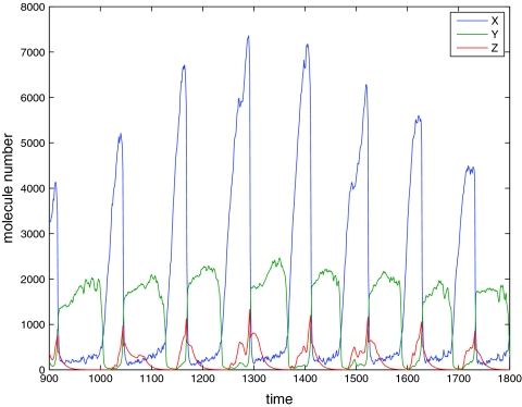
The hybrid cell cycle model can be naturally simulated by the hybrid method. The results are compared to the full Gillespie simulation on Kar et al.'s model (Figure 7 and Table 5). The hybrid model exhibits oscillations of the three proteins of X, Y, and Z (Figure 6) that are comparable to Kar et al.'s SSA results. The mRNA distributions of the hybrid method also agree quite well with Kar et al.'s calculation (Figure 7).

Figure 7.

mRNA distributions of the hybrid model with hybrid simulation and Kar's model with full SSA simulation.

Table 5.

Row 1 includes the experimental data from a fission yeast cell sample.¹¹ Row 2 includes the experimental data for daughter cells of the budding yeast.¹³ Rows 3 and 4 are statistics for the SSA on Kar's model and the hybrid method on the hybrid model, respectively.

	Cell cycle time		Volume at division
	Mean	CV	Mean	CV	CPU time
	(min)	(%)	(fl)	(%)	(s)
Fission yeast	116	14	175	8	…
Budding yeast (daughter)	112	22	68	19	…
Kar's	116	13	29	8	41 774
Hybrid	116	20	30	12	1370

Figure 6.

Time trajectory of the hybrid model.

Table 5 shows that the statistics generated by these two models agree reasonably well with each other and with the experimental data. Kar et al.'s model was parameterized to give a nominal size at division of 30 fl, without much regard for the actual size of yeast cells at division. This discrepancy can be corrected by adjusting the rate constants in Table 4. To increase V by a factor of F, k_dxy must be multiplied by F and all parameters with units fl⁻¹ or fl⁻¹ min⁻¹ must be divided by F.

Our hybrid model produces larger CVs of the cycle time and division size than Kar et al.'s model. Similar to Kar et al.'s model, our hybrid model includes low numbers of mRNAs. The average levels of M_x, M_y, and M_z are, respectively, 6.4, 2.0, and 0.5. With such low abundances, both models require short half-lives of the mRNAs in order to keep the intrinsic noise at an acceptable level. Therefore, we reuse the degradation rates of the mRNAs from Kar et al.'s model. The resulting half-lives of M_x, M_y, and M_z are, respectively, 0.2, 0.2, and 4.6 min, the same as in Kar et al.'s model. The hybrid model reduced the simulation time by a factor of 40. Moreover, from the modeling point of view, we avoid the difficulties that come from developing a complex chemical network, as in Kar et al.'s work.

ANALYSIS OF THE PARTITIONING STRATEGY

The numerical experiments of Kar et al.'s model suggest that the hybrid method with the new partitioning strategy can provide an accurate and efficient stochastic simulation for the cell cycle model. But, this may not be generally true for all types of models.

To further study the new strategy, we adopt a Poisson process formulation of the SSA proposed by Anderson.³⁴ Let k_j(t) denote the total number of firings for reaction R_j from initial time 0 to t. Then,

$$x\left(t\right)=x\left(0\right)+\sum _{j=1}^M{v}_j{k}_j\left(t\right).$$ (6)

Anderson³⁴ showed that k_j(t) can be formulated as

$$k_j\left(t\right)=Y_j\left({\int }_0^t{a}_j\left(x\left(s\right)\right)ds\right),$$ (7)

where all Y_j are independent unit-rate Poisson processes. Anderson called the integral $I_j\left(t\right)={\int }_0^t{a}_j\left(x\left(s\right)\right)ds$ the internal time, which determines the intensity inside a unit-rate Poisson process. I_j is also the time integral of the propensity function and determines the scale of the reaction R_j. Combining Eqs. 6, 7, we have

$$x\left(t\right)=x\left(0\right)+\sum _{j=1}^M{v}_j{Y}_j\left(I\left(t\right)\right).$$ (8)

Note that if we take the mean value for Y_j, we will end up with

$$x\left(t\right)=x\left(0\right)+\sum _{j=1}^M{v}_j\left({\int }_0^t{a}_j\left(x\left(s\right)\right)ds\right),$$ (9)

which is the integral format of the reaction rate equations. If we know the state at time t and would like to consider the state change from time t to t + h, we have

$$x(t+h)=x\left(t\right)+\sum _{j=1}^M{v}_j{P}_j\left({\int }_t^{t+h}{a}_j\left(x\left(s\right)\right)ds\right),$$ (10)

where all P_j(λ)'s are independent Poisson random numbers with mean and variance equal to λ. Note that although Eq. 10 looks similar to the tau-leaping method proposed by Gillespie,²⁵ it is an exact representation, while tau-leaping is an approximation.

Now consider different scenarios for a reaction R_j. If R_j is in region I or IV, the decision is relatively easy. In region I, at least one of the reactants/products is of small population and the reaction is slow. We should put this reaction into the SSA regime to exactly simulate its firing. In region IV, all reactants and products are of large populations and the reaction is fast. According to Haseltine and Rawlings,¹⁹ this reaction can be put into the ODE or the CLE regime. If R_j is in region II, all reactants and products of R_j are of large populations and the reaction is slow. Because the reaction is slow, ${\int }_t^{t+h}{a}_j\left(x\left(s\right)\right)ds$ is small and the corresponding Poisson random number cannot be approximated by either a normal random number or its mean value. However, since all the involved species are of large populations, the errors caused by the approximation are relatively small and will not affect the system behavior significantly. Even if we keep only the mean value and ignore the variance, the effect on the state variables is negligible. Thus, it is safe to put reactions from region II into the ODE or the CLE regime.³⁸

If R_j is in region III, there are species with large populations in reaction R_j. For them, the situation is similar to the case when R_j is in region IV. With fast reactions and species with large populations, there are no large errors in those species, if R_j is put into the ODE or CLE regime. But, since R_j is in region III, at least one of the reactants/products is of small population. Errors caused by an ODE or CLE approximation are relatively large in this case. Here, we do not aim to find general conditions such that R_j can be put into the ODE regime; instead, we focus on two conditions that suit our cell cycle model.

Condition 1: All chemical species of low molecular counts that participate in reactions within region III do not react with each other.

Condition 2: The sum of propensities for all reactions in region I is much smaller than the propensity of any reaction in region III.

Remark: For mass action kinetics, condition 1 guarantees that propensity functions of reactions involved with species of low populations are linear with the state variables corresponding to these species. Condition 2 requires that the total firing numbers in region I should not be comparable to the reacting number of any region II reaction. It is a necessary efficiency requirement since the efficiency of the hybrid method depends heavily on how frequently reactions in the SSA regime fire.

Assume that these two conditions are satisfied. Let the species with a small population be S_i, whose population x_i gets changed by a reaction R_j in region III. Then, v_ij ≠ 0. For x_i, we have

$$x_i\left(t\right)=x_i\left(0\right)+\sum _{j=1}^M{v}_{ij}{Y}_j\left(I_j\left(t\right)\right).$$ (11)

If I_j(t) is large, Y_j(I_j(t)) will also be large. But, since x_i is of small population, there must be at least a reaction R_l to change x_i in an opposite direction, in other words, v_ilv_ij < 0. We can rewrite Eq. 11 as

$$\begin{array}{ccc}\hfill x_i\left(t\right)& =& x_i\left(0\right)+\sum _{v_{i{j}^{\prime }}>0}{v}_{i{j}^{\prime }}{Y}_{j^{\prime }}\left({\int }_0^t{a}_{j^{\prime }}\left(x\left(s\right)\right)ds\right)\hfill \\ & & +\sum _{v_{i{j}^{\prime }}<0}{v}_{i{j}^{\prime }}{Y}_{j^{\prime }}\left({\int }_0^t{a}_{j^{\prime }}\left(x\left(s\right)\right)ds\right).\hfill \end{array}$$ (12)

Because of condition 2, it is impossible that reactions that change x_i in an opposite direction to R_j all come from region I. There must be at least a reaction R_l in region III such that v_ilv_ij < 0. Thus, x_i is changed by fast reactions in two directions, while it maintains a low population level. It has to be at a quasi-steady-state.^{27, 28, 33} According to the analysis by Rao and Arkin,²⁷ if x_i is involved only in reactions whose propensity functions are linear with the small state variables (condition 1), we only need its mean value to calculate the propensities of slow reactions, and its mean value can be solved from ODEs formed by those reactions in region III.

To see a counter example when condition 1 is broken, we consider a simple system

$$\begin{array}{ccc}\hfill X_1& \underset{c_2}{\overset{c_1}{\rightleftharpoons }}& X_2,\left(c_1=c_2=10000\right),\hfill \\ \hfill X_1+X_2& \stackrel{c_3}{\to }& X_3,(c_3=1).\hfill \end{array}$$ (13)

If both X₁ and X₂ have small populations, or in the extreme case where x₁ + x₂ = 1, then no X₃ will be produced since it is impossible that an X₁ molecule binds with an X₂ molecule to form an X₃ molecule. However, if we solve the pair of fast reversible equations using ODEs, we will have x₁(0.5) = x₂(∞) = 0.5 and there will be a positive propensity for the slow reaction. That will lead to errors.

If condition 2 is broken, we could have a system as follows:

$$\begin{array}{ccc}\hfill X_0& \stackrel{c_1}{\to }& \varnothing ,\text{with}{c}_1=2000\text{,}\hfill \\ \hfill X_i& \to & X_0+X_i,c_i=1,x_i=1,\hfill \\ & & \text{where}i=1,...,10000.\hfill \end{array}$$ (14)

The first reaction consumes X₀ quickly, while the other 10 000 reactions generate X₀ slowly. The first reaction is in region III and the other 10 000 reactions are in region I. For this system, x₀ will be around five at a steady state (since 5 × 2000 = 10 000). When we apply the hybrid method by solving the first reaction in ODEs and the rest in the SSA regime, the ODE solver will be interrupted by SSA events so frequently that the efficiency will be even lower than solving the whole system using the SSA.

Fortunately, conditions 1 and 2 are often satisfied in gene regulation networks, where proteins are of large populations, genes and mRNAs are of small populations, and reactions in region III are regulation reactions on genes and mRNAs by proteins. We note that the accuracy and efficiency of the hybrid method depend on the threshold values ($\overline{x}$ and $\overline{a}$ in Figure 2) and the actual scale differences in a problem. In general, it remains an open question how to select these threshold values. For Kar et al.'s model, the threshold values are determined so that all (and only) gene expression reactions are in the SSA regime. This seems to be a natural choice for gene regulation models where proteins, genes, and mRNAs demonstrate clear scale differences. To further test how this strategy works for this type of system, we did numerical experiments with two gene regulation models. One generates a steady state and the other generates an oscillation at the protein level. Details of these two models are given in the appendix. As shown by the experimental results, similar to what we have seen for Kar et al.'s model, the hybrid method with this partitioning strategy generates system dynamics and state statistics reasonably close to the SSA results for these two models as well.

CONCLUSION

Recent discoveries have shown that the cell cycle is characterized by different types of randomness, which play important roles in cell physiology.^{13, 35} Stochastic models of cell cycle regulation are necessary to understand these experimental results in quantitative terms. Kar et al. successfully converted Tyson and Novak's three-variable, deterministic, cell cycle model into a stochastic version by unpacking the phenomenological rate laws into detailed elementary reactions. However, this approach has serious costs. The largest cost is the time and effort needed to do the unpacking successfully. After that, there are computational expenses involved in full SSA-based simulations. These large costs make Kar et al.'s method hard to generalize to more complicated cell cycle models, such as Chen et al.'s budding yeast cell cycle model.⁹

In this paper, we have proposed to accelerate the stochastic simulation using Haseltine and Rawlings' hybrid method with a more efficient partitioning strategy. Through numerical experiments, we explored different partitioning strategies and concluded that, for certain classes of models, a reaction should be put into the SSA regime only when both of the following conditions are met: (1) the reaction has a relatively low average propensity; (2) at least one of its limiting species has a very low molecule number on average. This includes cell cycle models where, due to the low molecule numbers of genes and mRNAs, randomness mostly comes from reactions at the gene expression level. Our partitioning strategy also resulted in such a natural partitioning. Numerical experiments demonstrated that, with our new partitioning strategy, the hybrid method accurately simulates intrinsic noise with improved simulation efficiency. Although five-fold speedup does not seem to be significant at the first glance, the efficiency gain can be improved further with more efficient ODE solvers. LSODAR will have order and stepsize drops each time a SSA event fires. This is a great challenge for the implementation of the hybrid method. In the future, we will work on improving the ODE solver for the hybrid method.

A more serious difficulty with Kar et al.'s method is that it does not “scale up” easily to large deterministic models. For the simple cell cycle model with only three ODEs, the unpacked network required 19 variables and 47 reactions. For more realistic deterministic models, it may not be practical to unpack all the non-mass-action rate laws. To avoid this complexity, we propose a new way of building stochastic models of the cell cycle. Assuming most of the intrinsic noise comes from the gene expression level, we build stochastic reactions at the gene expression level and preserve the original phenomenological ODEs from the deterministic model. This combined model is self-partitioned and easily simulated by the hybrid method. Following this idea, we have successfully built a stochastic cell cycle model based on the original three-variable model of Tyson and Novak.⁷ In the future, we plan to investigate more complex and realistic models such as Chen et al.'s full model.⁹

APPENDIX: TEST OF THE PARTITIONING STRATEGY WITH TWO GENE REGULATION MODELS

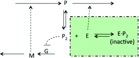
To test the accuracy of the hybrid method with the new partitioning strategy, we apply it to two gene regulation models. Their diagrams are shown in Figure 8.

Figure 8.

Diagrams for the two test models. The steady-state model does not include reactions in the shaded box, while the oscillation model includes them.

The first test case is a negative feedback model. The reactions are given in Table 6. In this model, a protein p regulates its own expression by forming a homodimer (p2), which binds to the promotor site of its own gene and inactivates gene expression. The average populations are set at typical values in cells. The reaction rates are chosen so that the model contains reactions in four regions.

Table 6.

Reactions in the steady-state model.

	Rate	Average no.	Average	Reaction
Reaction	constant	of molecules	propensity	region
g → g + m	2	10	1	I
m → m + p	0.1	1000	1	II
p → ϕ	0.001	1000	1	II
m → ϕ	0.1	10	1	I
p + p → p2	0.001	100	1000	IV
p2 → p + p	10	100	1000	IV
p2 + g → gi	20	0.5	1000	III
gi → p2 + g	2000	0.5	1000	III

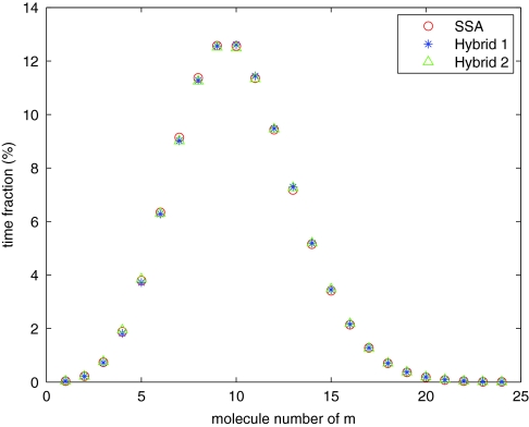
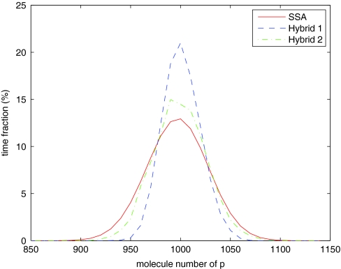
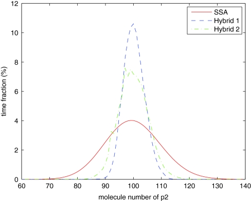
We simulate the system with three methods: the SSA, the hybrid method with only reactions in region I in the SSA regime, and the hybrid method with only reactions in region IV in the ODE regime. Note that for all methods, the distributions of the mRNA populations are similar (Figure 9). There are noticeable differences for the population distributions of the protein p (Figure 10) and its dimer p2 (Figure 11). But, the differences are actually typical for species with medium populations simulated by the hybrid method. We can see much higher differences for p2 as its population is one tenth that of p. Note that the mean values for both p and p2 are quite close to the SSA results.

Figure 9.

Distribution of mRNA population for the steady-state model.

Figure 10.

Distribution of p population for the steady-state model.

Figure 11.

Distribution of p2 population for the steady state model.

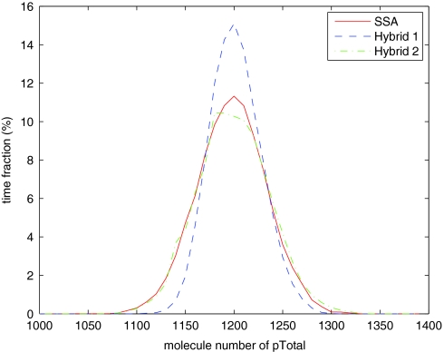
In many cases, the total protein level is more important than counts for phosphorylation level subpopulations, as the total is actually measured in wet-lab experiments. If we compare the distributions of the total protein population level pTotal = p + 2^*p2, they are much closer (Figure 12).

Figure 12.

Distribution of pTotal population for the steady state model.

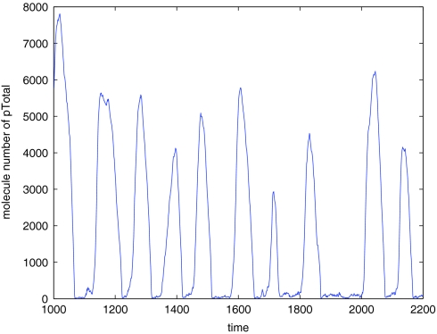
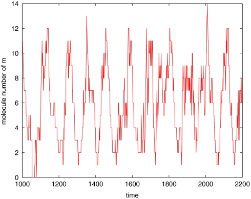
To determine how errors in protein level affect the accuracy of interesting system behaviors, we examined a second test case, an oscillation model. This model is an extension to the steady-state model. In this model, as before, protein p forms a homodimer, p2, which binds to the promotor region of the gene encoding p and inhibits the gene's expression. In addition, p2 binds to and inhibits the enzyme E that catalyzes the degradation of protein p. For a suitable choice of parameter values, this system exhibits spontaneous limit cycle oscillations³⁷ (see Figures 1314). The diagram is shown in Figure 8 and reactions are shown in Table 7. In the partitioning, species E has a relatively small population and the pair of reactions between E and p2 are relatively slow. But, they are still put into the ODE regime, and we expect some errors to result. The important characteristic for this system is the period of the oscillation. The statistics of the period by different simulation methods are shown in Table 8. We can see that the hybrid method with the new partitioning strategy works well for this model. With the original partitioning strategy, the accuracy of the hybrid method is almost the same as with the new partitioning strategy, but the CPU time is even greater than for the SSA. That is usually because of frequent firings of reactions in region III.

Figure 13.

Trajectory of pTotal in the oscillation model.

Figure 14.

Trajectory of mRNA in the oscillation model.

Table 7.

Reactions of the oscillation model.

	Rate	Average no.	Average	Reaction
Reaction	constant	of molecules	propensity	region
g → g + m	0.5	6.3	0.3	I
m → m + p	60	1439	375	IV
p → ϕ	0.05	1439	72	IV
m → ϕ	0.05	6.3	0.3	I
p + p → p2	0.001	120	4799	IV
p2 → p + p	40	120	4780	IV
p2 + g → gi	40	0.4	459	III
gi → p2 + g	1000	0.4	402	III
E + p2 → Ep2	0.4	23	22	IV
Ep2 → E + p2	0.5	23	23	IV
E + p → Ep	0.2	23	602	IV
Ep → E + p	10	23	300	IV
Ep → E	10	23	300	IV

Table 8.

Statistics for the period of oscillation for different methods simulating the stochastic oscillation model.

Simulation methods	Mean	CV	CPU time(s)
SSA	123	37%	37
Hybrid method with the new partitioning strategy	126	41%	0.8
Hybrid method with the original partitioning strategy	126	40%	40

References

- Hyver C. and Le Guyader H., Biosystems 24, 85 (1990). 10.1016/0303-2647(90)90001-H [DOI] [PubMed] [Google Scholar]
- Norel R. and Agur Z., Science 251, 1076 (1991). 10.1126/science.1825521 [DOI] [PubMed] [Google Scholar]
- Tyson J., Proc. Natl. Acad. Sci. U.S.A. 88, 7328 (1991). 10.1073/pnas.88.16.7328 [DOI] [PMC free article] [PubMed] [Google Scholar]
- Goldbeter A., Proc. Natl. Acad. Sci. U.S.A. 88, 9107 (1991). 10.1073/pnas.88.20.9107 [DOI] [PMC free article] [PubMed] [Google Scholar]
- Obeyesekere M., Herbert J., and Zimmerman S., Oncogene 11, 1199 (1995). [PubMed] [Google Scholar]
- Thron C., Biophys. Chem. 57, 239 (1996). 10.1016/0301-4622(95)00075-5 [DOI] [PubMed] [Google Scholar]
- Tyson J. and Novak B., J. Theor. Biol. 210, 249 (2001). 10.1006/jtbi.2001.2293 [DOI] [PubMed] [Google Scholar]
- Qu Z., Weiss J., and MacLellan W., Am. J. Physiol.: Cell Physiol. 284, C349 (2003). 10.1152/ajpcell.00066.2002 [DOI] [PubMed] [Google Scholar]
- Chen K., Calzone L., Csikasz-Nagy A., Cross F., Novak B., and Tyson J., Mol. Biol. Cell 15, 3841 (2004). 10.1091/mbc.E03-11-0794 [DOI] [PMC free article] [PubMed] [Google Scholar]
- Barberis M., Klipp E., Vanoni M., and Alberghina L., PLOS Comput. Biol. 3, e64 (2007). 10.1371/journal.pcbi.0030064 [DOI] [PMC free article] [PubMed] [Google Scholar]
- Miyata H., Miyata M., and Ito M., Cell Struct. Funct. 3, 39 (1978). 10.1247/csf.3.39 [DOI] [Google Scholar]
- Tyson J., BioEssays 2, 72 (1985). 10.1002/bies.950020208 [DOI] [Google Scholar]
- Di Talia S., Skotheim J., Bean J., Siggia E., and Cross F., Nature (London) 448, 947 (2007). 10.1038/nature06072 [DOI] [PubMed] [Google Scholar]
- Zenklusen D., Larson D., and Singer R., Nat. Struct. Mol. Biol. 15, 1263 (2008). 10.1038/nsmb.1514 [DOI] [PMC free article] [PubMed] [Google Scholar]
- Gillespie D., J. Comput. Phys. 22, 403 (1976). 10.1016/0021-9991(76)90041-3 [DOI] [Google Scholar]
- Gillespie D., J. Phys. Chem. 81, 2340 (1977). 10.1021/j100540a008 [DOI] [Google Scholar]
- Sabouri-Ghomi M., Ciliberto A., Kar S., Novak B., and Tyson J., J. Theor. Biol. 250, 209 (2008). 10.1016/j.jtbi.2007.09.001 [DOI] [PubMed] [Google Scholar]
- Kar S., Baumann W., Paul M., and Tyson J., Proc. Natl. Acad. Sci. U.S.A. 106, 6471 (2009). 10.1073/pnas.0810034106 [DOI] [PMC free article] [PubMed] [Google Scholar]
- Haseltine E. and Rawlings J., J. Chem. Phys. 117, 6959 (2002). 10.1063/1.1505860 [DOI] [Google Scholar]
- Tyson J. and Novak B., Curr. Biol. 18, R759 (2008). 10.1016/j.cub.2008.07.001 [DOI] [PMC free article] [PubMed] [Google Scholar]
- Thattai M. and Oudenaarden A., Proc. Natl. Acad. Sci. U.S.A. 98, 8614 (2001). 10.1073/pnas.151588598 [DOI] [PMC free article] [PubMed] [Google Scholar]
- Swain P., Elowitz M., and Siggia E., Proc. Natl. Acad. Sci. U.S.A. 99, 12795 (2002). 10.1073/pnas.162041399 [DOI] [PMC free article] [PubMed] [Google Scholar]
- Pedraza J. and Paulsson J., Science 319, 339 (2008). 10.1126/science.1144331 [DOI] [PubMed] [Google Scholar]
- Gillespie D., J. Chem. Phys. 113, 297 (2000). 10.1063/1.481811 [DOI] [Google Scholar]
- Gillespie D., J. Chem. Phys. 115, 1716 (2001). 10.1063/1.1378322 [DOI] [Google Scholar]
- Gillespie D. and Petzold L., J. Chem. Phys. 119, 8229 (2003). 10.1063/1.1613254 [DOI] [Google Scholar]
- Rao C. and Arkin A., J. Chem. Phys. 118, 4999 (2003). 10.1063/1.1545446 [DOI] [Google Scholar]
- Cao Y., Gillespie D., and Petzold L., J. Chem. Phys. 122, 014116 (2005). 10.1063/1.1824902 [DOI] [PubMed] [Google Scholar]
- Salis H. and Kaznessis Y., J. Chem. Phys. 122, 054103 (2005). 10.1063/1.1835951 [DOI] [PubMed] [Google Scholar]
- Salis H., Sotiropoulos V., and Kaznessis Y., BMC Bioinf. 7, 93 (2006). 10.1186/1471-2105-7-93 [DOI] [PMC free article] [PubMed] [Google Scholar]
- Cao Y., Gillespie D., and Petzold L., J. Chem. Phys. 123, 054104 (2005). 10.1063/1.1992473 [DOI] [PubMed] [Google Scholar]
- Gibson M. and Bruck J., J. Phys. Chem. 104, 1876 (2000). 10.1021/jp993732q [DOI] [Google Scholar]
- Cao Y., Gillespie D., and Petzold L., J. Comput. Phys. 206, 395 (2005). 10.1016/j.jcp.2004.12.014 [DOI] [Google Scholar]
- Anderson D., J. Chem. Phys. 128, 054103 (2008). 10.1063/1.2819665 [DOI] [PubMed] [Google Scholar]
- Skotheim J., Di Talia S., Siggia E., and Cross F., Nature (London) 454, 291 (2008). 10.1038/nature07118 [DOI] [PMC free article] [PubMed] [Google Scholar]
- Hindmarsh A. C., “ODEPACK, A systematized collection of ODE solvers,” in Scientific Computing, IMACS Transactions on Scientific Computation Vol. 1, edited by Stepleman R., Carver M., Peskin R., Ames W. F., and Vichnevetsky W. F. (North-Holland, Amsterdam, 1983), pp. 55–64. [Google Scholar]
- Novak B. and Tyson J. J., Nat. Rev. Mol. Cell Biol. 9, 981 (2008). 10.1038/nrm2530 [DOI] [PMC free article] [PubMed] [Google Scholar]
- Depending on the scale difference, one might want to put Rj into the tau-leaping regime. For simplicity, we only discuss using ODEs to simulate the fast reactions.