An S-System Parameter Estimation Method (SPEM) for Biological Networks

Abstract

Advances in experimental biology, coupled with advances in computational power, bring new challenges to the interdisciplinary field of computational biology. One such broad challenge lies in the reverse engineering of gene networks, and goes from determining the structure of static networks, to reconstructing the dynamics of interactions from time series data. Here, we focus our attention on the latter area, and in particular, on parameterizing a dynamic network of oriented interactions between genes. By basing the parameterizing approach on a known power-law relationship model between connected genes (S-system), we are able to account for non-linearity in the network, without compromising the ability to analyze network characteristics. In this article, we introduce the S-System Parameter Estimation Method (SPEM). SPEM, a freely available R software package (http://www.picb.ac.cn/ClinicalGenomicNTW/temp3.html), takes gene expression data in time series and returns the network of interactions as a set of differential equations. The methods, which are presented and tested here, are shown to provide accurate results not only on synthetic data, but more importantly on real and therefore noisy by nature, biological data. In summary, SPEM shows high sensitivity and positive predicted values, as well as free availability and expansibility (because based on open source software). We expect these characteristics to make it a useful and broadly applicable software in the challenging reconstruction of dynamic gene networks.

1. Introduction

Gene network inference, which aims to find interactions from biological data (Bansal et al., 2007), is among the most important and ambitious studies in modern systems and computational biology. With advances in the field of molecular biology, it is now possible to collect large quantities of gene-expression data, as well as to determine the change in gene-expression over a period of time, through the collection of times series data. Although of evident importance in determining the dynamic relationships between genes, which are often, by nature, non-linear (Voit, 1991), analysis of such time series data also allows us to determe how interactions change over time, important in the area of drug design, for example.

Currently, several models that are designed to reconstruct gene network structures from time series data exist. Generally, such models describe genetic networks as a set of differential equations:

(1)

where X_i is gene expression level of i-th gene, n the total number of genes in the network, and G_i a function used to describe the dynamic rule of gene regulatory interactions.

Different research groups adopt different approaches to model G_i. In addition to work that has assumed a simple Boolean (Akutsu et al., 2000) or a dynamic Bayesian (Geier et al., 2007; Yan et al., 2010) network structure, some authors (Kim et al., 2008; Kabir et al., 2010), have developed linear time-variant based models in order to successfully reconstruct non-linear connections in a network. Further, Kimura et al. (2008) used several power-law function approximates to solve this problem. Due to the ease in manipulating a non-linear relationship represented by power-laws to a more pliable linear function, power-laws lend themselves to use in reconstructing the non-linear networks that exist in biology.

Here, and expanding on work by others (Chou et al., 2006; Vilela et al., 2008; Voit and Radivoyevitch, 2000), we adopt an S-system (Voit, 2000; Maki et al., 2001; Chou and Voit, 2009) approach to represent biological networks, presenting a freely available package for the parameterization of biological networks from time series data alone (http://www.picb.ac.cn/ClinicalGenomicNTW/temp3.html).

S-systems, which have the fixed structure as shown in Equation 2, assume that the quantity (expression level) of each node (gene) in the network can be described, using power-laws, by the quantity of other nodes that it influences or that influence it (by activation or inhibition), coupled with the corresponding rate of each reaction.

(2)

where X_i is the expression level of the i-th gene and n the total number of genes in the network. α and β represent constant scale parameters, indicating the intensity of the relationship between gene X_i and other genes in the network. g_i,j and h_i,j are exponential parameters (referred to as kinetic orders), indicating the action of whether gene i activates or inhibits gene j, respectively.

Different approaches have been applied to estimate parameters in S-systems (Cho et al., 2006; Kimura et al., 2005; Gonzalez et al., 2007). In this article, we introduce an advanced method based on the S-system parameter optimization in Chou et al. (2006) and Vilela et al. (2008), in which the authors used eigenvector optimization of a matrix-representation of the system (A) from linearized noise-free time series data, combined with alternating regression, to estimate the constant rate parameters (α′s and β′s) and kinetic orders (g′s and h′s). Our method works directly on the logarithmic transition and its inverse matrix. In addition, as multiple S-systems can often represent the same set of time series data (i.e., the solution is not necessarily unique) we improve the method of Chou et al. (2006) and Vilela et al. (2008) by forcing sparsity into the system (Kikuchi et al., 2003), which we believe to be important in gene-network reconstruction. We argue that, although sparsity in a network is debatable, given the structure of known pathways, natural selection is indeed a mechanism that reduces gene interactions to a limited and often specific number of connections. For biological data, which are typically noisy, with many missing points, sparsity is a reasonable observation. Translation of this specificity in the mathematical concept of sparsity allows for one to reduce the number of unknowns in the equation and thus solve a system that would otherwise remain undetermined (di Bernardo et al., 2005; Gardner et al., 2003).

Under the aim of applying the method to biological analysis in particular, we proceeded to improve upon current models as follows:

• (1) Improvement of the slope calculation allows for noise in data (Varah, 1982; Voit and Savageau, 1982). The estimation of the slope (used in parameterisation of the system), is calculated, using the three-point method, directly from the input data, making it very sensitive to noise. To reduce sensitivity to noise, we have improved on other methods by (a) introducing a smoothing algorithm to minimise noise and (b) prediction of measurements at additional time points post-smoothing, to allow for a more accurate slope prediction.

• (2) To tackle the problem of identifying a unique solution, we use structure error (Kikuchi et al., 2003; Liu and Wang, 2008; Nelander et al., 2008) to force sparsity (Kikuchi et al., 2003) (by setting an adjustable threshold for the kinetic orders and forcing all kinetic orders whose absolute value is smaller than the threshold to be zero), thus also making it a closer match to biological systems. This approach has been applied to other algorithms (Liu and Wang, 2008), although here we continue to optimize the structure during the regression process.

To validate the improvement, the algorithm is tested on simulated data and on the Escherichia coli SOS pathway, the results of which show that our method is reliable, in particular regarding the directionality of the relationship between interacting genes. Driven by the common problem of having few time points per experiment (influencing the power of results and the ability of the algorithm to perform), we split the data into transitory and steady state stages, showing that the deletion of time points from the steady state phase has little effect on the results. The number of time points required in the transitory stage, for the algorithm to perform well, is determined.

2. Methods

2.1. Algorithm of SPEM

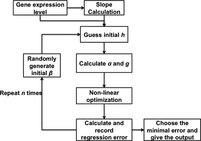
Based on the S-system approach in Chou et al. (2006) and Vilela et al. (2008), Figure 1 shows the flow chart of the algorithm, S-System Parameter Estimation Method (SPEM). The algorithm can be divided into estimation of the rate of change of expression (slope calculation) and optimization.

FIG. 1.

Main flow chart of SPEM.

2.1.1. Slope calculation

In S-system parameter estimation, the differential coefficient of each time point is calculated from a discrete dataset (Varah, 1982; Voit and Savageau, 1982; Voit and Almeida, 2004; Goel et al., 2008). This is non-trivial, as the estimation of the slope around any given time point t, which is based only on the time points t + 1 and t − 1, is sensitive to noise. Thus, in the collection of data that describe biological systems, where the distance between time points is often as sparse as reasonably possible, we are faced with the problem of relatively few time points and relatively high noise. In order to improve the ability of the three-point method (used here) to estimate a slope from the data, the data distribution was smoothed using spline interpolation (Hastie and Pregibon, 1992). This makes the point series denser, thus allowing for the slope, close to the original time points, to be estimated with more accuracy.

2.1.2. Optimization

The problem of network reconstruction is formulated as a function optimization problem aiming generally at the minimization of an objective function. This function is used to measure the goodness-of-fit of the model to the true system. Such a system may have multiple solutions, where different parameter values can lead to systems that are very “close” in nature. To mimic reality we must identify a unique solution that gives the most realistic model. In this direction, SPEM uses both square error, ε_squar, measuring the goodness-of-fit of the slope calculation, inferred from the data, to the data itself and structure error, ε_struc, which describes the (weighted) number or interactions in the network (used to force the predicted network to be sparse). In order for the numerical optimization process to run, SPEM calculates initial values for the kinetic orders h_i,j, using a pseudo-randomly generated value β_i > 0 and the expected slope, according to Equation 3. Note that in order to force the optimization to begin under the condition that α > 0, only the negative slope is considered

(3)

where ε → 0.

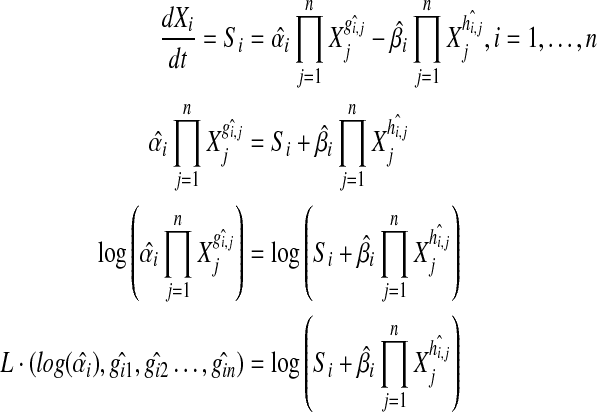
After fixing and , SPEM calculates the parameters and such that the change in expression of the i^th gene, , is described by Equation 4:

(4)

where N is the number of time points in the dataset and L equals:

Letting , then can be represented as::

(5)

Next, the expected slope for the i^th gene, is calculated as

(6)

And the squared error as:

(7)

Finally, it is necessary to force the gene interaction matrix to be sparse (as suggested in the introduction, this is more fitting to biological phenomena [di Bernardo et al., 2005; Gardner et al., 2003; Kikuchi et al., 2003]). Thus, we introduce structure error for sparsity control, as in Nelander et al. (2008). For a given gene i, the structure error ε_struc, which depends only on the number of interactions in a network, can be defined as the total number of non-zero elements in and .

The non-linear optimization function (solved using Rsolnp, R v2.12 [Ye, 2010]) can then be described as:

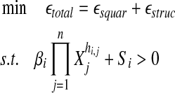(8)

Table 1 shows the input parameters and output parameters used by SPEM.

Table 1.

Input and Output of Our Algorithm SPEM

Input parameters
TS	Time series data matirx, columns for genes and rows for expression level on different time points
tp	Timp points, an increasing non-negative vector
n	Positive value, SPEM will guess initial β for n times. (Note to keep n small to improve running time.)
thres	Interactions with absolute value smaller than thres will be set to zero
lbH,ubH,lbB,ubB	Lower boundary value, upper boundary value for h and β, respectively
Output parameters
α, g, β, h	Parameter of the reconstructed S-system
IniBeta	Estimate of the initial β
error	Regression error

SPEM, S-System Parameter Estimation Method.

2.2. Validation

2.2.1. Benchmark validation

In this work, we focus on the edges in the network, which represent the interactions between genes. Let matrix A represent the gene interaction matrix for n genes, with elements representing the edges of the network. In general, a gene network can be undirected, directed, unsigned, or signed (Bollobás, 1998).

Assessment of the performances of an algorithm is usually done by defining positive (P) and negative (N) in the result of the algorithm and true (T) and false (F) in the gold standard (a model from which simulated data are generated, or an interaction matrix collected from literature and validated by experiments). In case of signed networks, the definitions of T, F, N, and P require an extension due to the presence of positives and negative values (+1, −1) (Nardini et al., 2009).

Here, we present results on directed networks only. Since directed networks contain more information and are thus harder to predict than undirected networks, we report on the performance of both signed and unsigned cases. In this work, to account properly for the signed performances, we use the R package MultiClassTest (http://cran.r-project.org/) to calculate the positive predictive value (PPV) for precision and sensitivity (Se) for recall of the performance of our algorithm, where PPV and Se are defined as:

(9)

The area under the curve (AUC) of the PPV/Se curve, which plots the performances of the algorithm on matrices, filtered according to a range of different thresholds, is used as a summary statistic. We use AUC value to find a balance of precision and recall of our algorithm.

2.2.2. Requirement of the time points

In order to achieve a reliable result, also appropriate in experimental design, it is important to determine how many time points are required by SPEM for accurate reconstruction of the gene network. As points in the transitory state contain more information than points in the steady state, we will discuss the two states separately.

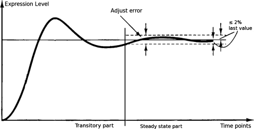
Figure 2 shows how we define the transitory and steady states. After smoothing of the gene expression curve, we give an adjustment error δ equal to 2% of the last value of the time series. (The value of 2% as a measurement of error is borrowed from control theory [Ogata, 2001].) In the event that the last value is zero, which implies the gene is not expressed, then the transitory part in SPEM would contain all non-zero expression levels of that gene. We judge the transitory state based on the value of each point compared to the last point in the time series, as this distance determines the trend of the curve—and hence the system.

FIG. 2.

Example of how to distinguish between the transitory and steady states of a curve. Here, we set an adjustment error equal to the 2% of the last value. The system is assumed to be in the transitory state until the time after which all remaining measurements are in the range of last value ± adjust error.

3. Results and Discussion

3.1. Results for noise free synthetic data.

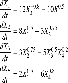
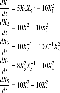
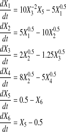
We generated noise free time series data for didactic systems (also lacking slope error) of 4, 5, and 6 genes using Power Law Analysis and Simulation (PLAS) Version 1.0, according to Equations 10, 11, and 12. For comparison, datasets with four and five genes match those in Chou et al. (2006) and Vilela et al. (2008).

(10)

(11)

(12)

Table 2 shows the initial value of all X_is, as well as all α_is, β_is, g_i,js and h_i,js as reconstructed by SPEM. From the table, we see that for datasets with four and six genes, SPEM obtains perfect results. However, for the dataset containing five genes, only two genes were predicted without error.

Table 2.

Performance of Noise Free Data

Four-gene dataset
	α	g1	g2	g3	g4	β	h1	h2	h3	h4	Initial value
Gene1	11.99	0	0	−0.8	0	9.99	0.49	0	0	0	0.1
Gene2	7.99	0.5	0	0	0	3	0	0.75	0	0	0.1
Gene3	3	0	0.75	0	0	4.99	0	0	0.5	0.2	0.1
Gene4	2	0.49	0	0	0	6	0	0	0	0.8	0.1

Five-gene dataset
	α	g1	g2	g3	g4	g5	β	h1	h2	h3	h4	h5	Initial value
Gene1	7.42	−0.127	0	1.32	−0.55	−0.28	10	0	0.48	0	0	0	0.1
Gene2	10	2	0	0	0	0	10	0	1	0	0	0	0.7
Gene3	10.7	0.3	2.2	2.3	0.67	1.4	10	0.38	−2.2	−2.2	0.63	1.5	0.7
Gene4	8	0	0	1.99	0	−0.99	10	0	0	0	1.99	0	0.16
Gene5	10	−0.29	0.7	0.6	2.5	−1.87	10	−0.25	0.67	0.6	0.1	0.66	0.18

Six-gene dataset
	α	g1	g2	g3	g4	g5	g6	β	h1	h2	h3	h4	h5	h6	Initial value
Gene1	10	0	0	−2	0	1	0	5	0.5	0	0	0	0	0	1.1
Gene2	5	0.5	0	0	0	0	0	10	0	0.5	0	0	0	0	0.5
Gene3	2	0	0.5	0	0	0	0	1.25	0	0	0.5	0	0	0	0.9
Gene4	8	0	0.5	0	0	0	0	5	0	0	0	0.5	0	0	0.75
Gene5	0.5	0	0	0	0	0	0	1	0	0	0	0	0	1	0.5
Gene6	1	0	0	0	0	0	1	0.5	0	0	0	0	0	0	0.75

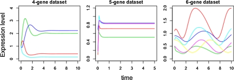
In order to further understand this phenomenon, consider the expression curves of these three datasets: Figure 3 shows that those datasets with four genes and six genes contain more information in the transitory state than that of five genes. Not only does X₂ in the third equation have the same power in both terms (Function 11), which may be the cause of the problem, we also notice that in the five-gene data set, the steady state is quickly reached, thus masking information that might occur in the transitory state (i.e., too few measurements were taken in the transitory state to describe the dynamics of the system). Thus, for expression data that contain little information, there may exist a higher number of possible solutions, reducing the power of the algorithm to determine the correct solution. The amount of data that is required to achieve an acceptable level of accuracy is explored.

FIG. 3.

Pictorial representation of synthetic datasets with four, five, and six genes (from left to right). Curves show how the expression level of each gene changes over the time period studied. Note that for the five-gene dataset, only the first 50 time points are shown, in order to show clarity in the transitory state.

3.2. Time point requirements

In order to explore how many data points are required in the transitory and steady states, for accurate results to be obtained two additional datasets, each with four genes and with different initial values (Table 3), were generated according to Function 10. Points were then deleted in the transitory and steady states in order to investigate the change in the performance of SPEM, given different quantities of data.

Table 3.

Expression Level for Genes (X_i) at Time = 0 (Initial Value)

Initial condition	X1(0)	X2(0)	X3(0)	X4(0)
1	0.10	0.10	0.10	0.10
2	0.10	3.0	1.3	0.13
3	1.5	0.5	0.5	1.5

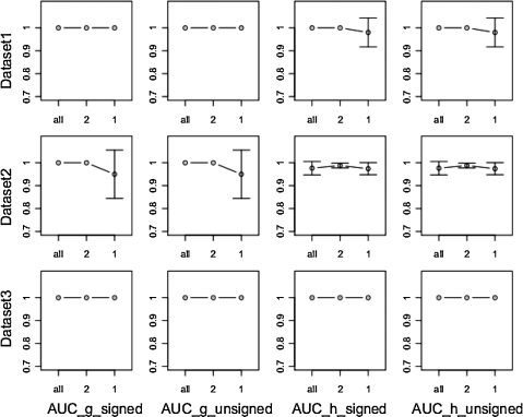
Data collected when the system is in its steady state contain little additional information and collection of too many measurements in this state defeats one of the advantages of collecting time series data, by wasting resources. We therefore tested SPEM on data containing one or two points in the steady state and all original points in the transitory state. Figure 4 shows the performance of SPEM, measured using the AUC value. The results show that when we have only one point from the steady state, an AUC value of 1 is still obtained. SPEM thus requires little information from the steady state in order to achieve accurate results.

FIG. 4.

Area under curve (AUC) value of SPEM results on a four-gene system, under different initial conditions (Dataset 1–3) and different network types (signed or unsigned). The AUC value (of both signed and unsigned) of g and h were tested separately for all points, two points, and one point in the steady state.

We then tested the time points needed in the transitory state using only one time point in the steady state phase. The number of time points in the transitory state, before removal of data, were 68, 64, and 62, in datasets 1, 2, and 3, respectively. We compared the results obtained when all points were considered with 3/4 of all points, 1/2 of all points, and 1/4 of all points (Fig. 5). Figure 5 shows that datasets 1 and 3 require only 34 and 31 transitory points for an AUC value of 1 to be obtained, but dataset 2 is quite different. When 32 of the transitory points are removed from dataset 2, the AUC value is close to 0.95, and in fact, the AUC value already begins to drop when as many as 48 of the points remain. When 17, 16, and 15 of the points remain, the AUC value for datasets 1 and 3 falls to approximately 0.95, implying that removing this many points is too many. The reduction in the number of points in the transitory part of dataset 2 (compared to 1 and 3) may cause the reduction in accuracy for dataset 2. Further, this low number of points in the transitory part may also cause an instability in the non-linear optimization function, Rsolnp. Determining the true effect of this on the optimization algorithm is highlighted as an area of further study. We speculate that one possible explanation relates to the situation in which the problem is highly non-linear or non-smooth. In this case, it is possible to have many local solutions, resulting in the function becoming “trapped.”

FIG. 5.

Area under curve (AUC) value of SPEM results on a four-gene system, under different initial conditions (Dataset 1–3) and different network types (signed or unsigned). The AUC value (of both signed and unsigned) of g and h were tested separately for all points, 3/4, 1/2, and 1/4 of points in the transitory state.

We infer that, for SPEM to solve a system, few time points are needed in the steady state but one should obtain 20–25 measurements in the system's transitory state in order to achieve accurate results. Determining the sensitivity of this number to n, for example, is highlighted here as an area of further study (Goel et al., 2008). In order for this important results to be efficiently used in experimental design, advice from experimental biologists on when a steady state is likely to be reached is required.

3.3. Result for SOS

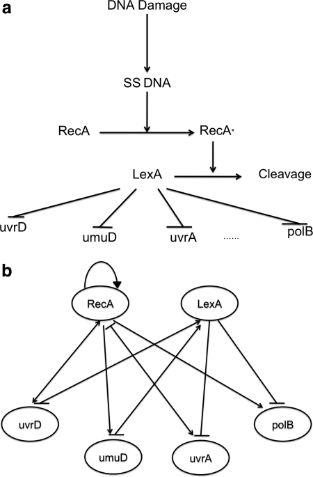
Reiterating that real biological data contain noise, we applied SPEM to the E. coli SOS DNA repair system. The dataset is described as a time-course gene-expression matrix, containing many zeros. As reported by existing literature, LexA and RecA are hub genes in the regulatory SOS pathway (they connect many other genes) and are bound to the interaction sites of other genes as master repressors. The data used here describes the reactions directly related to these two hub genes (download from the Uri Alon lab: http://www.weizmann.ac.il/mcb/UriAlon/). Although the downloaded dataset contains eight genes (uvrD, lexA, umuD, recA, uvrA, uvrY, ruvA, and polB) taken from Experiment 3 (UV light intensities, 4:20 Jm⁻²), here we chose to compare results for the same six genes investigated in Kimura et al. (2008, 2009) and Kabir et al. (2010) (uvrD, lexA, umuD, recA, uvrA, and polB). In this way, a fair comparison between SPEM and other published results can be performed. These six genes are in fact well studied, and the network of interactions can be described as in Figure 6a (Ronen et al., 2002).

FIG. 6.

SOS DNA repair pathway in Escherichia coli: (a) According to the literature. (b) As predicted by SPEM.

Figure 6b shows the regulatory network as reconstructed by SPEM. Comparing with Figure 6a, we see that SPEM correctly predicted all of the (activation) reactions related to RecA as well as all of the (inhibition) reactions of LecA, including reaction direction. Intriguingly, the only true reaction that SPEM did not predict was the reaction that occurs between RecA and LexA.

The performance of SPEM is compared, using the gold standard (Table 4), to other published algorithms by considering the PPV and Se of the algorithm on signed and unsigned versions of the SOS pathway. The results (Table 5) show that SPEM performs better here than in other approaches, in terms of both PPV (0.62) and Se (0.65) in the signed network, with the next best algorithm for the signed network being that published in Kabir et al. (2010), where PPV = 0.39 and Se = 0.35. For the unsigned network, SPEM has the highest PPV (0.71 compared to 0.67 in Kabir et al. [2010] and Kimura et al. [2009]) and the second highest Se (0.75, compared to 0.8 in Kimura et al. [2009]).

Table 4.

Gold Standard of SOS Pathway, Collected from the Literature

	uvrD	lexA	umuD	recA	uvrA	polB
uvrD	0	−1 (Gardner et al., 2003; Ronen et al., 2002)	−1 (Kato and Shinoura, 1977; Steinborn, 1978)	1 (Gardner et al., 2003; Ronen et al., 2002)	1 (Szklarczyk et al., 2011)	0
lexA	0	−1 (Gardner et al., 2003; Ronen et al., 2002)	−1 (Gardner et al., 2003)	1 (Gardner et al., 2003; Ronen et al., 2002)	0	0
umuD	0	−1 (Gardner et al., 2003; Ronen et al., 2002)	−1 (Gardner et al., 2003)	1 (Gardner et al., 2003; Ronen et al., 2002)	0	0
recA	0	−1 (Gardner et al., 2003; Ronen et al., 2002)	−1 (Gardner et al., 2003)	1 (Gardner et al., 2003; Ronen et al., 2002)	0	0
uvrA	1 (Szklarczyk et al., 2011)	−1 (Gardner et al., 2003; Ronen et al., 2002)	−1 (Kato and Shinoura, 1977; Steinborn, 1978)	1 (Gardner et al., 2003; Ronen et al., 2002)	0	0
polB	0	−1 (Gardner et al., 2003; Ronen et al., 2002)	−1 (Kato and Shinoura, 1977; Steinborn, 1978)	1 (Gardner et al., 2003; Ronen et al., 2002)	0	0

Table 5.

Comparison of SPEM with Other Published Algorithms on SOS Pathway

	Signed		Unsigned
	PPV	Se	PPV	Se
SPEM	0.62	0.65	0.71	0.75
Kimura2008 (Kimura et al., 2008)	0.33	0.35	0.52	0.55
Kimura2009 (Kimura et al., 2009)	0.167	0.2	0.67	0.8
Kabir2010 (Kabir et al., 2010)	0.39	0.35	0.67	0.6

SOS: a global response pathway to DNA damage in which the cell cycle is arrested and DNA repair and mutagenesis are induced.

Results of other algorithms are taken directly from the corresponding literature.

SPEM, S-System Parameter Estimation Method; SOS, …

Bold values are for emphasis.

These results are of particular interest because they show that SPEM is able to perform well on real, and therefore noisy data, and better, or comparably well, than existing approaches on the same dataset. As the noise problem has not been clearly discussed in other approaches, we believe that, in our comparison, one of the reasons that SPEM is superior to other methods is its efficient noise processing.

4. Conclusion

In this article, we have presented an algorithm for the estimation of parameters in an S-system, from time series data. The algorithm, SPEM, is an improvement on algorithms that have previously been published in the field of reverse-engineering of gene networks as it uses structural error to effectively force sparsity into the (biological) network, and importantly, it is able to process noisy data through improved slope calculation. This means that SPEM performs well on real, as well as synthetic, data. Although we acknowledge that SPEM cannot give 100% accurate results every time (see Section 3.2), the algorithm has high levels of Se and PPV for the networks studied. In addition, SPEM is designed so that the user can change parameters such as the level of required sparsity, allowing for prior knowledge to be accounted for if desired.

If the number of time points and number of genes are high, SPEM will be time costly (Goel et al., 2008). To minimize this, we have used vector computation instead of loop computation, and the current version supports parallel computation. One feasible improvement is embedded parallel computation on the code itself, and this improvement is planned in an update of SPEM.

Another natural stage in development of SPEM would be to allow for the time series input data to include perturbations at arbitrary time points. In addition, it would be of interest to investigate other options for introducing sparsity into the networks, thus potentially decreasing runtime of the algorithm. One could adopt ideas from LARS (least angle regression) (Efron et al., 2004), based on the Lasso approach (Tibshirani, 1996) to allow for sparsity. However, to date, LARS can deal only with optimization of linear models, GLMs, and Cox proportional hazard models (see packages LARS and glmpath in R [Friedman et al., 2008]). We therefore highlight the extension of LARS to S-system parameterization as a potential area for future study.

Acknowledgments

This work was funded by the National Science Foundation of China (NSFC; grant 31070748).

Disclosure Statement

No competing financial interests exist.

References

- Akutsu T. Miyano S. Kuhara S. Algorithms for identifying Boolean networks and related biological networks based on matrix multiplication and fingerprint function. J. Comput. Biol. 2000;7:331–343. doi: 10.1089/106652700750050817. [DOI] [PubMed] [Google Scholar]
- Bansal M. Belcastro V. Ambesi-Impiombato A., et al. How to infer gene networks from expression profiles. Mol. Syst. Biol. 2007:3. doi: 10.1038/msb4100120. [DOI] [PMC free article] [PubMed] [Google Scholar]
- Bollobás B. Modern Graph Theory. Vol. 184. Springer Verlag; New York: 1998. [Google Scholar]
- Cho D. Cho K. Zhang B. Identification of biochemical networks by S-tree based genetic programming. Bioinformatics. 2006;22:1631–1640. doi: 10.1093/bioinformatics/btl122. [DOI] [PubMed] [Google Scholar]
- Chou I. Voit E. Recent developments in parameter estimation and structure identification of biochemical and genomic systems. Math. Biosci. 2009;219:57–83. doi: 10.1016/j.mbs.2009.03.002. [DOI] [PMC free article] [PubMed] [Google Scholar]
- Chou I. Martens H. Voit E.O. Parameter estimation in biochemical systems models with alternating regression. Theor. Biol. Med. Model. 2006;3:25. doi: 10.1186/1742-4682-3-25. [DOI] [PMC free article] [PubMed] [Google Scholar]
- di Bernardo D. Thompson M.J. Gardner T.S., et al. Chemogenomic profiling on a genome-wide scale using reverse-engineered gene networks. Nat. Biotechnol. 2005;23:377–383. doi: 10.1038/nbt1075. [DOI] [PubMed] [Google Scholar]
- Efron B. Hastie T. Johnstone I., et al. Least angle regression. Ann. Stat. 2004;32:407–499. [Google Scholar]
- Friedman J. Hastie T. Tibshirani R. Sparse inverse covariance estimation with the graphical lasso. Biostatistics. 2008;9:432. doi: 10.1093/biostatistics/kxm045. [DOI] [PMC free article] [PubMed] [Google Scholar]
- Gardner T. di Bernardo D. Lorenz D., et al. Inferring genetic networks and identifying compound mode of action via expression profiling. Science. 2003;301:102. doi: 10.1126/science.1081900. [DOI] [PubMed] [Google Scholar]
- Geier F. Timmer J. Fleck C. Reconstructing gene-regulatory networks from time series, knock-out data, and prior knowledge. BMC Syst. Biol. 2007;1:11. doi: 10.1186/1752-0509-1-11. [DOI] [PMC free article] [PubMed] [Google Scholar]
- Goel G. Chou I. Voit E.O. System estimation from metabolic time-series data. Bioinformatics. 2008;24:2505. doi: 10.1093/bioinformatics/btn470. [DOI] [PMC free article] [PubMed] [Google Scholar]
- Gonzalez O.R. Küper C. Jung K., et al. Parameter estimation using simulated annealing for S-system models of biochemical networks. Bioinformatics. 2007;23:480–486. doi: 10.1093/bioinformatics/btl522. [DOI] [PubMed] [Google Scholar]
- Hastie T. Pregibon D. Statistical Models in s. Wadsworth & Brooks/Cole; New York: 1992. [Google Scholar]
- Kabir M. Noman N. Iba H. Reverse engineering gene regulatory network from microarray data using linear time-variant model. BMC Bioinform. 2010;11:S56. doi: 10.1186/1471-2105-11-S1-S56. [DOI] [PMC free article] [PubMed] [Google Scholar]
- Kato T. Shinoura Y. Isolation and characterization of mutants of Escherichia coli deficient in induction of mutations by ultraviolet light. Mol. Gen. Genet. 1977;156:121–131. doi: 10.1007/BF00283484. [DOI] [PubMed] [Google Scholar]
- Kikuchi S. Tominaga D. Arita M., et al. Dynamic modeling of genetic networks using genetic algorithm and S-system. Bioinformatics. 2003;19:643–650. doi: 10.1093/bioinformatics/btg027. [DOI] [PubMed] [Google Scholar]
- Kim J. Bates D.G. Postlethwaite I., et al. Linear time-varying models can reveal non-linear interactions of biomolecular regulatory networks using multiple time-series data. Bioinformatics. 2008;24:1286–1292. doi: 10.1093/bioinformatics/btn107. [DOI] [PubMed] [Google Scholar]
- Kimura S. Ide K. Kashihara A., et al. Inference of S-system models of genetic networks using a cooperative coevolutionary algorithm. Bioinformatics. 2005;21:1154–1163. doi: 10.1093/bioinformatics/bti071. [DOI] [PubMed] [Google Scholar]
- Kimura S. Sonoda K. Yamane S., et al. Function approximation approach to the inference of reduced NGnet models of genetic networks. BMC Bioinform. 2008;9:23. doi: 10.1186/1471-2105-9-23. [DOI] [PMC free article] [PubMed] [Google Scholar]
- Kimura S. Nakayama S. Hatakeyama M. Genetic network inference as a series of discrimination tasks. Bioinformatics. 2009;25:918–925. doi: 10.1093/bioinformatics/btp072. [DOI] [PubMed] [Google Scholar]
- Liu P. Wang F. Inference of biochemical network models in S-system using multiobjective optimization approach. Bioinformatics. 2008;24:1085–1092. doi: 10.1093/bioinformatics/btn075. [DOI] [PubMed] [Google Scholar]
- Maki Y. Tominaga D. Okamoto M., et al. Development of a system for the inference of large-scale genetic networks. Pac. Symp. Biocomput. 2001;6:446–458. doi: 10.1142/9789814447362_0044. [DOI] [PubMed] [Google Scholar]
- Nardini C. Wang L. Peng H., et al. MM-Correction: meta-analysis-based multiple hypotheses correction in omic studies, 242–255. In: Fred A., editor; Filipe J., editor; Gamboa H., editor. Biomedical Engineering Systems and Technologies. Vol. 25. Springer; Berlin: 2009. [Google Scholar]
- Nelander S. Wang W. Nilsson B., et al. Models from experiments: combinatorial drug perturbations of cancer cells. Mol. Syst. Biol. 2008;4:216. doi: 10.1038/msb.2008.53. [DOI] [PMC free article] [PubMed] [Google Scholar]
- Ogata K. Modern Control Engineering. Prentice Hall PTR; Englewood Cliffs, NJ: 2001. [Google Scholar]
- Ronen M. Rosenberg R. Shraiman B. I., et al. Assigning numbers to the arrows: parameterizing a gene regulation network by using accurate expression kinetics. Proc. Natl. Acad. Sci. USA. 2002;99:10555–10560. doi: 10.1073/pnas.152046799. [DOI] [PMC free article] [PubMed] [Google Scholar]
- Steinborn G. UVM mutants of Escherichia coli k12 deficient in UV mutagenesis. I. Isolation of UVM mutants and their phenotypical characterization in DNA repair and mutagenesis. Mol. Gen. Genet. 1978;165:87–93. doi: 10.1007/BF00270380. [DOI] [PubMed] [Google Scholar]
- Szklarczyk D. Franceschini A. Kuhn M., et al. The string database in 2011: functional interaction networks of proteins, globally integrated and scored. Nucleic Acids Res. 2011;39:D561. doi: 10.1093/nar/gkq973. [DOI] [PMC free article] [PubMed] [Google Scholar]
- Tibshirani R. Regression shrinkage and selection via the lasso. J. Roy. Stat. Soc. B Met. 1996:267–288. [Google Scholar]
- Varah J. A spline least squares method for numerical parameter estimation in differential equations. SIAM J. Sci. Stat. Comput. 1982;3:28. [Google Scholar]
- Vilela M. Chou I. Vinga S., et al. Parameter optimization in S-system models. BMC Syst. Biol. 2008;2:35. doi: 10.1186/1752-0509-2-35. [DOI] [PMC free article] [PubMed] [Google Scholar]
- Voit E. Canonical Nonlinear Modeling: S-System Approach to Understanding Complexity. Van Nostrand Reinhold; New York: 1991. [Google Scholar]
- Voit E. Computational Analysis of Biochemical Systems: A Practical Guide for Biochemists and Molecular Biologists. Cambridge University Press; New York: 2000. [Google Scholar]
- Voit E. Almeida J. Decoupling dynamical systems for pathway identification from metabolic profiles. Bioinformatics. 2004;20:1670. doi: 10.1093/bioinformatics/bth140. [DOI] [PubMed] [Google Scholar]
- Voit E.O. Radivoyevitch T. Biochemical systems analysis of genome-wide expression data. Bioinformatics. 2000;16:1023–1037. doi: 10.1093/bioinformatics/16.11.1023. [DOI] [PubMed] [Google Scholar]
- Voit E. Savageau M. Power-low approach to modeling biological systems. II. Application to ethanol production. J. Ferment. Technol. 1982;60:229–232. [Google Scholar]
- Yan W. Zhu H. Yang Y., et al. Effects of time point measurement on the reconstruction of gene regulatory networks. Molecules. 2010;15:5354–5368. doi: 10.3390/molecules15085354. [DOI] [PMC free article] [PubMed] [Google Scholar]
- Ye Y. Interior algorithms for linear, quadratic, and linearly constrained non linear programming [Ph.D. dissertation] Stanford University; Stanford, CA: 2010. [Google Scholar]